Synthetic Optimization of Trafficability and Roll Stability for Off-Road Vehicles Based on Wheel-Hub Drive Motors and Semi-Active Suspension

Abstract

Considering the requirements pertaining to the trafficability of off-road vehicles on rough roads, and since their roll stability deteriorates rapidly when turning violently or passing slant roads due to a high center of gravity (CG), an efficient anti-slip control (ASC) method with superior instantaneity and robustness, in conjunction with a rollover prevention algorithm, was proposed in this study. A nonlinear 14 DOF vehicle model was initially constructed in order to explain the dynamic coupling mechanism among the lateral motion, yaw motion and roll motion of vehicles. To acquire physical state changes and friction forces of the tires in real time, corrected LuGre tire models were utilized with the aid of resolvers and inertial sensors, and an adaptive sliding mode controller (ASMC) was designed to suppress each wheel’s slip ratio. In addition, a model predictive controller (MPC) was established to forecast rollover risk and roll moment in reaction to the change in the lateral forces as well as the different ground heights of the opposite wheels. During experimentation, the mutations of tire adhesion capacity were quickly discerned and the wheel-hub drive motors (WHDM) and ASC maintained the drive efficiency under different adhesion conditions. Finally, a hardware-in-the-loop (HIL) platform made up of the vehicle dynamic model in the dSPACE software, semi-active suspension (SAS), a vehicle control unit (VCU) and driver simulator was constructed, where the prediction and moving optimization of MPC was found to enhance roll stability effectively by reducing the length of roll arm when necessary.

1. Introduction

Benefiting from eminent responsiveness and precision compared to conventional hydraulic or mechanical systems, various electrified chassis assemblies, such as electric independent drive systems (EIDS), steering-by-wire systems (SBWS), and electronically controlled suspension systems (ECSS), have been widely researched. Diverse stability optimization methods have been proposed based on these advanced techniques, as vehicle attitude can be directly corrected by adjusting the torque in different directions. Active yaw moment (AYM) is expected to better improve the handling stability and maneuverability of vehicles. Model predictive control (MPC) has also been widely used in vehicle control systems in recent years, and better dynamic control performance can be obtained by using rolling optimization strategies. Therefore, in various studies, output torque difference between contralateral drive motors and active steering control have been applied to correct vehicle trajectory [1,2,3,4,5,6,7,8,9,10]. However, irregular roads and different adhesion limits of the four tires were not taken into account in the aforementioned studies. Furthermore, the restraint of slip ratio, rather than lateral stability and maneuverability, should serve as the primary objective when driving on rough or variable adhesion roads at a relatively low velocity.

In order to suppress the power wastage of the drive system and improve trafficability, a robust and rapid-update identification method of adhesion coefficient ($\mu$) is necessary. Researchers have estimated according to real-time updated measurement data from inertial measurement unit (IMU), GPS and extended Kalman filter [11,12,13], which demonstrated credible results through scrupulous verifications. However, the disparities of the wheels’ slip ratios, which have become more distinct in off-road conditions, and the independent torque control of the four driving wheels were neglected in these studies. The LuGre tire model was proposed to estimate the adhesive conditions online [14], unlike empirical formula tire models whose characteristic parameters were difficult to iterate. Here, the tire forces were calculated based on the measured tire–road contact surface (TRCS) deformation along with the rotational speeds of the driving wheels. Three-axis accelerometers were installed on the inner surfaces so as to capture the tangential, radial and lateral deformations of TRCS, so the angle of slip of the tire slip angle was able to be computed online in the LuGre tire model [15,16]. To constrain the angular velocities of the unloaded wheels while enhancing lateral stability, a new approach that combines the practical proportional-integral-derivative (PID) controller and Fuzzy-logic controller (FLC) has been extensively employed in the anti-lock braking system (ABS) and Traction Control System (TCS) [17,18,19,20], though it is subject to defects that inaccurately adjust the feature parameters. However, PID and FLC are inappropriate for use in strongly nonlinear off-road environments.

Active Stability Control (ASC) may be easily activated under intense steering intentions or driving on snow-covered or muddy roads as the adhesion limits of the four wheels vary greatly. Furthermore, the lateral motion can become abruptly violent due to the increase in velocity and steering angle. According to certain studies on vehicle roll stability, a close-knit coupling relationship between rollover risk and lateral acceleration [21,22]. Off-road vehicles and trucks, particularly those with high CG, were more likely to roll over and cause lethal accidents [23,24]. Simultaneously, in order to enhance the roll stability, responsiveness, and ride comfort of vehicles, some scholars have endeavored to integrate modern control technologies such as PID, backstepping control, sliding mode control, and fuzzy algorithms, with the aim of improving the maneuverability and safety of vehicles in complex road conditions [25,26].

To prevent such vehicles from rolling over, the predictive load transfer ratio (PLTR) was explored to express the rollover risk and make the ECSS an actuator to control the roll angle (Ω) and roll rate ($\dot{\Omega }$) under the drastic steering input [27]. In addition to ECSS, various studies have analyzed yaw-roll coupled motion and have optimized multidimensional dynamic stability based on active aerodynamic control (AAC), active differential braking (ADB), EIDS, SBWS and ECSS [28,29,30,31]. Furthermore, the physical properties may influence the roll motion, such as the great unsprung masses (m_ui) caused by WHDM [32] as well as the response hysteresis of ADB [33], which have been evaluated.

In summary, considering the advantage of independently controllable torque for each wheel in hub motor-driven off-road vehicles, and the current research on optimal traction torque control and road adhesion estimation being limited to flat roads with-out taking into account tire adhesion limits and roll passability on irregular road surfaces. Therefore, to further optimize the off-road capability and roll stability of hub motor-driven off-road vehicles, an in-depth analysis will be conducted on optimal traction torque control and tire adhesion limits on irregular road surfaces. The purpose of this paper is mainly to improve the robustness of distributed drive off-road vehicles and develop electric control algorithms to achieve the passing performance of the complex drive train (inter-axle differential lock, driveshaft, electro-hydraulic braking system) of conventional off-road vehicles. The goal is to optimize the coordination of each electric wheel assembly under varying four-wheel attachment conditions and drastic changes in working conditions. To accommodate the strong disturbances of nonpaved roads that are imposed on different tires, an adhesion state monitor comprised of the LuGre tire model, resolvers and inertial sensor was proposed, in which an ASMC is adopted to improve the driving-power utilization rate (DPURi) based on the four WHDMs to realize the fast and smooth convergences of slip-ratio in off-road conditions. Additionally, a nonlinear 14 DOF vehicle model was established to estimate load transfer ratio (LTR) over a finite-time horizon in an MPC to avoid rollover in advance by adjusting the model of SAS. During the experiment, the designed ASC was tested under various typical off-road conditions, where trafficability was analyzed quantitatively. Furthermore, the feasibility of rollover prevention when passing sharp slants was validated on the HIL platform.

This paper is organized as follows: Section 2 presents the theoretical dynamic model, which includes the nonlinear 14 DOF vehicle model and LuGre tire model. The coordination control module i described in Section 3, which includes off-road vehicle and off-road vehicle stability. Real vehicle and HIL tests are presented in Section 4. The concluding remarks are presented in Section 5.

2. The Theoretical Dynamic Model

A nonlinear 14 DOF vehicle model with a front steer system was initially established in order to analyze the coupling relationships among different motions along and around the multi-axis of the vehicle body. Next, a corrected LuGre tire model was built, in which the control modules were given access to acquire normal loads, contact states, and friction forces of the four wheels. Since observations were made in real time for vehicle motions, both the responsiveness and robustness of rollover prevention and slip-ratio suppression controllers were considered credible.

2.1. Subsection

A 14 DOF vehicle model that considers the vehicle longitudinal, lateral, and yaw motions in the X–Y planes, as well as the vertical, roll and pitch motions of $m_s$ and the vertical, and rotational motions of the four wheels, was adopted to dissect the coupling relationships between the active chassis units and vehicle stability in multiple directions, the nonlinear 14 DOF vehicle dynamic model is shown in Figure 1. The interpretation of the computational variables in this paper is shown in

Table 1. Explanation of some computational variables in the vehicle dynamic model.

Explanation	Variables	Unit
The vehicle total mass	m	kg
Unsprung masses	mui, (i = FL, FR, RL, RR)	kg
Sprung masses	msi, (i = FL, FR, RL, RR)	kg
Front wheel steering angle	${\delta }_i$, (i = FL, FR)	deg
Yaw rate of CG in the vehicle body coordinate system	γ	deg/s
Sideslip angle of CG in the vehicle body coordinate system	β	deg
Yaw angle of vehicle in the geodetic coordinate system	ψ	deg
Heading angle of vehicle in the geodetic coordinate system	Ω	deg
Roll angle of the sprung mass	ϕ	deg
Pitch angle of the sprung mass	θ	deg
Steering angle of the front wheel	δ	deg
The rotational inertia of the vehicle mass around the Z-axis of CG	Iz	kg·m2
The rotational inertia of the sprung mass around the X-axis of CG	IxC	kg·m2
The inertia product of sprung mass around the X-axis and Z-axis of CG	IxzC	kg·m2
The rotational inertias of sprung mass around X-axis	IxS	kg·m2
The rotational inertias of sprung mass around X-axis	IxS	kg·m2
The rotational inertias of the sprung mass around Y-axis	IyS	kg·m2
The rotational inertias of the sprung mass around Z-axis	IzS	kg·m2
The stiffness factors of four suspensions	Ksi, (i = FL, FR, RL, RR)	-
The damping factors of four suspensions	Csi, (i = FL, FR, RL, RR)	-
The equivalent stiffness of four tires	Kti, (i = FL, FR, RL, RR)	N·m
The output torques of four WHDM	Twi, (i = FL, FR, RL, RR)	N·m
The vertical displacements of four unsprung masses	Zui, (i = FL, FR, RL, RR)	mm
The vertical displacements of four sprung masses	Zsi, (i = FL, FR, RL, RR)	mm
The vertical displacements of four contact patches	Z0i, (i = FL, FR, RL, RR)	mm
The height of roll center	h	mm
The height of sprung mass’s barycenter	hm	mm
The arm length of roll moment	hs	mm
Track width	tw	mm
The heights of four tires ground positions	hZi, (i = FL, FR, RL, RR)	mm
Gravity acceleration	g	m/s2

.

As described in the models in Figure 1, the motion status was decomposed into three planes. To represent vehicle stability in the X–Y plane, the geodetic coordinate system ($x_G-y_G$) and vehicle body coordinate system ($x_V-y_V$) were applied to describe γ, ψ, Ω, β, a_y and a_x:

$$a_x={\dot{V}}_{xV}-V_{yV}\gamma$$

(1)

$$a_y={\dot{V}}_{yV}+V_{xV}\gamma \approx V_{xV}(\dot{\beta }+\gamma )$$

(2)

$$\{\begin{array}{c}\psi =\int \gamma dt\\ \beta =\mathsf{\Omega }-\psi \end{array}$$

(3)

In addition, a_x and a_y can be expressed according to longitudinal and lateral tire forces:

$$m{a}_x=\left(F_{xFL}+F_{xFR}\right)\cos \delta -(F_{yFL}+F_{yFR})\sin \delta +F_{xRL}+F_{xRR}$$

(4)

$$m{a}_y=\left(F_{xFL}+F_{xFR}\right)\sin \delta +(F_{yFL}+F_{yFR})\cos \delta +F_{yRL}+F_{yRR}$$

(5)

The effects of driving/braking and suspension assemblies acting on the roll, pitch motions of carriage, and vehicle yaw motion should also be analyzed. As shown in Figure 1a, the yaw motion was expounded as the moment equation around the Z-axis of the CG:

$$\begin{array}{l}{I}_z\dot{\gamma }+(\dot{\theta }\gamma -\ddot{\varphi })I_{xzC}+(I_{yS}-I_{xS})\dot{\theta }\dot{\varphi }=[(F_{yFL}+F_{yFR})\cos \delta +\\ (F_{xFL}+F_{xFR})\sin \delta ]L_F-(F_{yRL}+F_{yRR})L_R+\frac{t_w}{2}[(F_{yFL}-F_{yFR})\sin \delta +\\ (F_{xFR}+F_{xFL})\cos \delta +F_{xRR}-F_{xRL}]\end{array}$$

(6)

The left side of (6) expresses that the yaw moment created by the friction forces of the four tires affects the lateral stability and indirectly changes the angle of motion and roll angles of the carriage. Evidently, the lateral instability would make the shift of CG and vehicle attitude increasingly difficult to control. Therefore, limiting the tire friction’s movement may be fatal in stability optimization.

In Figure 1, the roll-motion of m_s as elaborated in the Y-Z plane, in which the roll rate was calculated as:

$$\begin{array}{l}{I}_{xC}\ddot{\varphi }+\left(m_s{h}_s{h}_m+I_{yS}-I_{zS}\right)\gamma \dot{\theta }-I_{xzC}\dot{\gamma }=\\ m_{s}g{h}_s\left(a_{y}cos\varphi +gsin\varphi \right)+\frac{t_w}{2}\left(F_{zSFL}-F_{zSFR}+F_{zSRL}-F_{zSRR}\right)\end{array}$$

(7)

Equation (7) further illustrates that the steady lateral motion contributes to roll stability, where the normal forces F_zSi (i = FL, FR, RL, RR) between the suspension system and m_s in (7) were expected to rapidly respond to the change in roll moment:

$$F_{zSi}=K_{si}\left(z_{ui}-z_{si}\right)+C_{si}\left({\dot{z}}_{ui}-{\dot{z}}_{si}\right)$$

(8)

$$K_{si}\left(z_{ui}-z_{si}\right)+C_{si}\left({\dot{z}}_{ui}-{\dot{z}}_{si}\right)+m_{ui}{\ddot{z}}_{ui}-K_{ti}\left(z_{0i}-z_{ui}\right)=0$$

(9)

To facilitate the study and establishment of the corresponding simulation model, the characteristics of the spring and damping elements are considered to be linear in this paper. As demonstrated in Figure 1c and Equation (9), $K_{si}$ and $C_{si}$ should be greater in order to improve the responsiveness of the suspension system to roll motion. However, these parameters should be kept within limits considering the influence of vertical acceleration on ride comfort.

2.2. Tire Model

The tire is the only component that is directly affected by road friction forces and moments transmitted by the suspension system, steering mechanism, driving system, and braking devices. To enhance the credibility of the estimated motion status, various tire models were applied to acquire the tire forces and moments. Empirical/semi-empirical formula tire models were introduced to verify the other models’ accuracy as many test data of the tire’s mechanical property were obtained during the tire design process, though they were different since the theoretical tire models calculated the friction forces by measuring physical deformations. Deeded as the offline models, the empirical formula tire models were unable to update the fitted curves to fit the disturbances from the actual scenario. The characteristic parameters of the theoretical tire models, however, may adapt to the great external disturbance, assuming some specific kinematics messages are able to be acquired in real time.

The precision is difficult to maintain when four tires in adhesive conditions change instantaneously; thus, modified models like SWIFT were used to analyze the tire’s transient dynamic characteristics of the tire through the groundmass block slip model. The LuGre tire model does not merely describe the elastic deformations of TRCS but also considers the correlation between relative velocity and frictional characteristics. Accordingly, the changes in tire forces could be seized without much test data if the rotational speeds and normal loads are measurable on the onboard sensors, including the resolver, inertial sensor, triaxial accelerometer, and so forth. To adapt to the intense environment noise, a dynamic LuGre tire model with a higher renewal frequency and inferior calculative expense was established to assess the adhesive state of each tire. The advantage of the LuGre tire model is that it responds quickly and can quickly identify the step change in the adhesion limit of each wheel. Its model parameters are calibrated based on the magic tire model and tire parameters. The schematic formulas are expressed as:

$$\dot{z}=V_r-\epsilon \frac{{\sigma }_0\left|V_r\right|}{g\left(V_r\right)}z$$

(10)

$$m\dot{V}=\left({\sigma }_0\mathrm{z}+{\sigma }_1\dot{z}+{\sigma }_2{V}_r\right)F_{zS}$$

(11)

$$T_w=J\dot{w}+\left({\sigma }_0\mathrm{z}+{\sigma }_1\dot{z}\right)r_w{F}_{zS}+{\sigma }_{w}w$$

(12)

$$\mathrm{g}\left(V_r\right)={\mu }_c+\left({\mu }_s-{\mu }_c\right)e^{-{\left|V_r/V_s\right|}^{1/2}}$$

(13)

where z signifies the tire grounded length, ε shows the variation in pavement condition, $V_r(=r_{w}w-V)$ is the relative velocity between the tire and contact patch, $r_w$ is wheel radius, $w$ is wheel angular velocity, $V$ is wheel center velocity, $g(V_r)$ is the sliding friction function describing the change in friction force with diverse lubrication conditions, $T_w$ is wheel torque, $J$ is wheel moment of inertia, ${\sigma }_0$ is the normalized rubber lumped stiffness, ${\sigma }_1$ is the normalized rubber lumped damping, ${\sigma }_2$ is the normalized viscous relative damping, ${\mu }_c$ is the normalized coulomb friction coefficient, ${\mu }_s$ is the normalized static friction coefficient, $Vs$ is the trick relative velocity, and ${\sigma }_w$ denotes the viscous rotational friction. To acquire the change in a tire’s adhesion condition, a state space observer was devised to estimate the vertical load, inertial loss and actual driving torque of the tire depending on the above formulas:

$$\{\begin{array}{c}{\dot{x}}_i=A{x}_i+B\left({\epsilon }_i\frac{{\sigma }_0\left|V_{ri}\right|}{g\left(V_{ri}\right)}{z}_i\right)+E{y}_i+F{u}_i\\ y_i=C{x}_i\end{array}$$

(14)

Here, the state vector is $x_i={\left[x_1 x_2 x_3\right]}^T={\left[z_i \left(r_w{F}_{zSi}{\sigma }_1{z}_i+J_w{w}_i\right) \left(J_w{w}_i+m_i{r}_{w}V\right)\right]}^T$. ${\dot{x}}_i$ describes the tire’s vertical deformation, the moment of inertia and effective wheel torque. Since the variables $y_i=w_i(i=FL,FR,RL,RR)$ were measured using the WHDM resolvers and torques of WHDM, $u_i=T_{wi}$ can be accurately adjusted by the current control. ${\dot{x}}_i$ was obtained directly, and the formulas of $x_2$, $x_3$ were acquired by integrating (11) into (12), from which the following characteristic matrixes were derived:

$$A=\left[\begin{array}{ccc}0& 0& \frac{-1}{r_w{m}_i}\\ 0& \frac{-{\sigma }_0}{{\sigma }_1}& 0\\ 0& 0& \frac{-F_{zSi}{\sigma }_2}{m_i}\end{array}\right],B=\left[\begin{array}{c}-1\\ 0\\ 0\end{array}\right],C={\left[\begin{array}{c}\frac{-r_w{F}_{zSi}{\sigma }_1}{J_w}\\ \frac{1}{J_w}\\ 0\end{array}\right]}^T,E=\left[\begin{array}{c}\frac{r_w^2{m}_i+J_w}{r_w{m}_i}\\ \frac{J_w{\sigma }_0-{\sigma }_1{\sigma }_w}{{\sigma }_1}\\ \left(\frac{J_w+m_i{r}_w^2}{m_i}\right)F_{zSi}{\sigma }_2-{\sigma }_w\end{array}\right],F=\left[\begin{array}{c}0\\ 1\\ 1\end{array}\right]$$

where m_i is the proportion of the vehicle’s mass in the wheels; J_w is moment of inertia of each wheel; the rank of the augmented matrix (A, C) was not less than three and the system was observable.

In this study, $w_i$ was measured using the resolvers embedded in WHDM, and the V output of the Global Position System (GPS) served as the credible variable to assess the estimation error of ε. Concurrently, $F_{ni}$ was calculated using the metrical data from the inertial sensor fastened to the steady-state CG. Accordingly, the estimation state-space function was listed as:

$$\{\begin{array}{c}{\dot{\widehat{x}}}_i=A{\widehat{x}}_i+B\left[{\widehat{\epsilon }}_i\frac{{\sigma }_0\left|{\widehat{V}}_{ri}\right|}{g\left({\widehat{V}}_{ri}\right)}{\widehat{z}}_i+O_1\right]E{y}_i+F{u}_i+K{\tilde{y}}_i\\ {\dot{\widehat{\epsilon }}}_i=-O_2\end{array}$$

(15)

To build the estimator of $\epsilon$, two active adaptive laws, $O_1$ and $O_2$, was utilized to evaluate the convergence rate of ${\dot{\widehat{\epsilon }}}_i$. Additionally, $K={[k_1,k_2,k_3]}^T$ served as a positive constant vector. Subtracting (15) from (14), the changes in estimated errors were obtained, and the actual adhesion condition was transiently stable as ${\dot{\widehat{\epsilon }}}_i$ was equal to zero.

$$\{\begin{array}{c}{\dot{\widehat{x}}}_i=\left(A-KC\right){\tilde{x}}_i+B\left[{\epsilon }_i\frac{{\sigma }_0\left|V_{ri}\right|}{g\left(V_{ri}\right)}{z}_i-{\widehat{\epsilon }}_i\frac{{\sigma }_0\left|{\widehat{V}}_{ri}\right|}{g\left({\widehat{V}}_{ri}\right)}{\widehat{z}}_i+O_1\right]\\ {\dot{\widehat{\epsilon }}}_i=O_2\end{array}$$

(16)

A Lyapunov function was defined, in which the following stability criterion should be met:

$$V_{LuGre}={\tilde{\epsilon }}_i^2+{\tilde{x}}_i^{T}P{\tilde{x}}_i$$

(17)

P denotes a real symmetric matrix, and $P>0,PB=C$; $(A-KC)$ was restrained by the transfer function between state variables and estimation errors:

$${\theta }_i={\epsilon }_i\frac{{\sigma }_0\left|V_{ri}\right|}{g\left(V_{ri}\right)}{z}_i-{\widehat{\epsilon }}_i\frac{{\sigma }_0\left|{\widehat{V}}_{ri}\right|}{g\left({\widehat{V}}_{ri}\right)}{\widehat{z}}_i+O_1$$

(18)

$$G\left(s\right)=\frac{{\tilde{y}}_i\left(s\right)}{{\theta }_i\left(s\right)}$$

(19)

$G(s)$ can be calculated based on the matrixes A, B, and C.

$$G\left(s\right)=C{\left[Is+KC-A\right]}^{-1}B$$

(20)

The characteristic equation of $G(s)$ was obtained:

$$s^2+\left(\frac{F_{zSi}{\sigma }_2-k_3{r}_w{F}_{zSi}{\sigma }_1}{m_i{J}_w}\right)s\frac{k_1{F}_{zSi}{\sigma }_1-k_3{r}_w{F}_{zSi}^2{\sigma }_1{\sigma }_2}{m_i{J}_w}=0$$

(21)

The vector K should satisfy $k_1>0$ and $k_3<0$ to obtain the real characteristic roots of the negative parts. Additionally, $\exists Q>0$, $\left|Q\right|=q$ satisfied the criterion $P\left[A-KC\right]+{\left[A-KC\right]}^{T}P=-Q$, after which the derivative of $V_{LuGre}$ can be obtained:

$${\dot{V}}_{LuGre}=-{\tilde{x}}_i^{T}Q{\tilde{x}}_i+2{\tilde{\epsilon }}_i\left[{\tilde{y}}_i\frac{{\sigma }_0\left|{\widehat{V}}_{ri}\right|}{g\left({\widehat{V}}_{ri}\right)}{\widehat{z}}_i+O_2\right]+2{\tilde{y}}_i{\epsilon }_i\left[\frac{{\sigma }_0\left|V_{ri}\right|}{g\left(V_{ri}\right)}{z}_i-\frac{{\sigma }_0\left|{\widehat{V}}_{ri}\right|}{g\left({\widehat{V}}_{ri}\right)}{\widehat{z}}_i\right]+2{\tilde{y}}_i{O}_1$$

(22)

The adaptive law $O_2=-{\tilde{y}}_i\frac{{\sigma }_0\left|{\widehat{V}}_{ri}\right|}{g\left({\widehat{V}}_{ri}\right)}{\widehat{z}}_i$ and $\left|{\epsilon }_i\right|$ is not greater than ${\epsilon }_{max}$. Hence, $\frac{{\sigma }_0\left|V_{ri}\right|}{{\mu }_c}\left|z_i\right|\le \frac{{\sigma }_0\left|w_{max}\right|}{{\mu }_c}\left|z_{max}\right|=f_{max}$ and ${\dot{V}}_{LuGre}\le -q{\left|\left|{\tilde{x}}_i\right|\right|}^2+2\left|{\tilde{y}}_i\right|\left[{\epsilon }_{max}\left(f_{max}-\frac{{\sigma }_0\left|{\widehat{V}}_{ri}\right|}{g\left({\widehat{V}}_{ri}\right)}{\widehat{z}}_i\right)+sgn\left({\tilde{y}}_i\right)O_1\right]$ were tenable. Next, $O_1$ and the observation function were determined under the convergence condition ${\dot{V}}_{LuGre}\le -q{\left|\left|{\tilde{x}}_i\right|\right|}^2$:

$$O_1=-{\epsilon }_{max}\left(f_{max}-\frac{{\sigma }_0\left|{\widehat{V}}_{ri}\right|}{g\left({\widehat{V}}_{ri}\right)}{\widehat{z}}_i\right)sgn\left({\tilde{y}}_i\right)$$

(23)

$$\{\begin{array}{c}{\dot{\widehat{z}}}_i={\widehat{V}}_{ri}-{\widehat{\epsilon }}_i\frac{{\sigma }_0\left|{\widehat{V}}_{ri}\right|}{g({\widehat{V}}_{ri})}{\widehat{z}}_i-k_1{\widehat{y}}_i+O_1\\ {\widehat{\epsilon }}_i=\frac{{\sigma }_0\left|{\widehat{V}}_{ri}\right|}{g({\widehat{V}}_{ri})}{\widehat{z}}_i{\tilde{y}}_i\\ {\dot{\tilde{w}}}_i=\frac{T_{wi}-{\sigma }_w{w}_i-F_{zSi}{r}_w({\sigma }_0{\widehat{z}}_i+{\sigma }_1{\widehat{z}}_i)}{J_w}\\ r_w{m}_i\dot{\widehat{V}}=T_{wi}+{\sigma }_2{F}_{zSi}{r}_w{\widehat{V}}_{ri}-{\sigma }_w{w}_i-J_w{\dot{\widehat{w}}}_i+k_3{\tilde{y}}_i\end{array}$$

(24)

${\widehat{\epsilon }}_i$ was obtained by integrating ${\dot{\widehat{\epsilon }}}_i$ that mutated with the drastic increase in $\left|{\dot{w}}_i\right|$. Hence, the decrease in maximal tire friction forces may be supervised forthwith. To eliminate the distortion of integration due to the accumulation of measurement errors and slight road disturbance, a specific calculation rule of ${\epsilon }_i$ was proposed on the basis of $\tilde{y}$:

$$\{\begin{array}{c}If O{S}_i=0\cup \tilde{y}<{\tilde{w}}_{i1}:{\epsilon }_i={\epsilon }_{i0}\\ Else if O{S}_i=0\cup \tilde{y}\ge {\tilde{w}}_{i1}:O{S}_i=1\\ If O{S}_i=1\cup \tilde{y}\ge {\tilde{w}}_{i2}:{\epsilon }_i={\epsilon }_{i0}+\int \dot{\widehat{\epsilon }}dt\\ Else if O{S}_i=1\cup \tilde{y}<{\tilde{w}}_{i2}:O{S}_i=0\end{array}$$

(25)

where ${\epsilon }_{i0}=1$ and ${\tilde{w}}_{i2}<{\tilde{w}}_{i1}$.

3. The Coordination Control Module

In addition to the dynamic tire model, the robust controllers and the driving system possessed great accuracy and responsiveness, which were essential in boosting $DPU{R}_i$ in off-road conditions. Consequently, ASMC was constructed in this study to confine the four wheels’ slip ratio (${\lambda }_i=1-\left(v_x/r_w{w}_i\right)$) and rely on WHDMs. Additionally, SAS was used to straightly adjust the tires’ vertical loads of the tires by lowering the height of CG if the rollover risk could not be neglected. To modify the integrated control effect of $DPU{R}_i$ and roll stability, an MPC was proposed to coordinately control WHDM and SAS. The logic diagram of this control module is described in Figure 2.

3.1. Off-Road Vehicle

The effective exertion of the wheel attachment abilities emphasized trafficability optimization. $DPU{R}_i$ was acquired based on the LuGre tire model to appraise the effect of the torque regulator in a timely manner.

In order to suppress ${\lambda }_i$ on rough roads, low-adhesion roads and soft ground, mechanical differential locks (MDL) that realize the inter-axial torque distribution through various locking devices, as well as electrical differential locks (EDL) that control the hydraulic brake system to suppress wheel speed differences, were generally used in the off-road vehicles. Engine output moment can be transferred to load wheels, and the drive-power loss was decreased significantly when MDL was enabled. However, the vehicle would be anchored if the torque transfer angle and torsion deformations of the driving shafts were violent. Since the driving torque was evenly distributed to the opposite wheels via a differential mechanism, EDL applied extra hydraulic braking forces suppressing ${\lambda }_i$ were applied by EDL by sacrificing driving efficiency. Moreover, $w_i$ would have fluctuated greatly due to the violent torque regulation and response hysteresis of EDL.

As WHDM only transmits torque to the wheel through a planetary reducer integrated within the rim, the mechanical transmission was decoupled from the sprung mass while the torque transfer angle was effectively confined. In the present research, the three-phase current of the permanent magnet synchronous motor (PMSM) was accurately adjusted by the vector control and inverters, hence the speeds of the unloaded or low-adhesion wheels were restrained solely by reducing the quadrature axis current of WHDM.

To ensure ${\lambda }_i$ was within the linear range, ${\mu }_i$ served as the most critical adhesion state parameter, which was also presented in numerous studies. The second-order sliding mode controller (SOSMC) based on supertwisting algorithm was built in [34] to reduce lateral offset and heading angle deviation against a great $\left|{\dot{\mu }}_i\right|$, but the measurement of chassis velocity and ${\dot{F}}_{zi}$ was not appreciated. Moreover, the accuracy of estimated ${\mu }_i$ as well as the adaptability of off-road conditions was accordingly restricted. The moment transfer process was considered in [35], while the open-loop transfer function of the driving torque was built to avoid the online estimation of ${\mu }_i$. Furthermore, the stable region of the tire was discerned according to ${\dot{\lambda }}_i$. In terms of a off-road vehicle, ${\dot{F}}_{zi}$ should be promptly detected, and a quick response feedback loop is essential.

$DPU{R}_i$ was obtained and regulated by the LuGre tire model’s output variables as well as the driving force transfer process, where the control target of ASC was then calculated. Accordingly, an ASMC along with its sliding surface was proposed.

${\lambda }_i$ is regarded as a function of two variables ($v_x,w_i$), thus, ${\dot{\lambda }}_i\left(v_x,w_i\right)$ is figured up. Additionally, the driving force transfer process under acceleration operation can be expressed in different ways:

$$\{\begin{array}{c}{\dot{\lambda }}_i=\frac{\partial {\lambda }_i}{\partial v_x}{a}_x+\frac{\partial {\lambda }_i}{\partial w_i}{\dot{w}}_i=\frac{v_x}{r_w{w}_i^2}{\dot{w}}_i-\frac{a_x}{r_w{w}_i}\\ r_w{\dot{F}}_{xi}=i_m{\dot{T}}_i-J_i\frac{d}{dt}{\dot{w}}_i \\ {\dot{F}}_{xi}=f_i{F}_{zi}{\dot{\lambda }}_i \\ {\dot{F}}_{xi}=F_{zi}{\dot{a}}_x \end{array}$$

(26)

where $i_m$ is the motor reduction ratio, $J_i$ is moment of inertia of each wheel, ${\dot{F}}_{xi}$ was calculated by the torque balance equation $i_m{T}_i=r_w{F}_{xi}+J_i{\dot{w}}_i$ and Newton’s second law $F=ma$, which can be estimated by the fitted curve of ${\mu }_i\left({\lambda }_i\right)$. The transfer function $L\left(r_w{\dot{F}}_{xi}/\dot{T}\right)$ was acquired according to the Laplace transformation:

$$i_{m}L\left({\dot{T}}_i\right)=\left(\frac{J_i{w}_i}{\left(1-{\lambda }_i\right)r_w{f}_i{F}_{zi}}\right)L\left(r_w{\dot{F}}_{xi}\right)s+\frac{J_i}{r_w^2{F}_{zi}\left(1-{\lambda }_i\right)}L\left(r_w{\dot{F}}_{xi}\right)+L\left(r_w{\dot{F}}_{xi}\right)$$

(27)

In view of analyzing the stability of the torque control system intuitively, $L\left(r_w{\dot{F}}_{xi}\right)$ was expressed in the format $L\left(x\right)=K/\left({\tau }_n{s}^n+{\tau }_{n-1}{s}^{n-1}+\dots +{\tau }_{1}s+1\right)$ based on (27):

$$\{\begin{array}{c}L\left(\frac{r_w{\dot{F}}_{xi}}{{\dot{T}}_i}\right)=\frac{K_{di}\left(k\right)}{{\tau }_{di}\left(k\right)s+1}\\ K_{di}\left(k\right)=i_m-\frac{i_m{J}_w}{J_i+r_w^2{F}_{zi}\left(k\right)\left(1-{\lambda }_i\left(k\right)\right)}\\ {\tau }_{di}\left(k\right)=\frac{J_w{r}_w{w}_i}{f_i\left(J_i+r_w^2{F}_{zi}\left(k\right)\left(1-{\lambda }_i\left(k\right)\right)\right)}\end{array}$$

(28)

${\tau }_{di}\left(k\right)$ was greater than zero as $\left(1-{\lambda }_i\right)>0$, hence the transfer function possessed a negative real root, and the system was stable.

${\dot{T}}_i$ is decided by the driver’s acceleration instruction, the peak current of WHDM, and the adjusted torque of ASC ($\Delta T_i$). The state variables update during each acceleration pedal sampling period of the accelerator pedal (${\tau }_{acc}$). Moreover, ${\dot{T}}_{Wi}$ is influenced by the communication delay of the CAN bus and the response delay of the inverters, thus ${\dot{T}}_{Wi}\left({\dot{T}}_i\right)$ is simplified as a first-order damp system whose delay time is ${\tau }_W$:

$${\dot{T}}_i\left(k\right)=\{\begin{array}{c}\frac{F_{zi}{\dot{\alpha }}_{acc}\left(k\right)T_{maxi}\left(k\right)}{mg},O{S}_i=0\\ \frac{F_{zi}{\dot{\alpha }}_{acc}\left(k\right)T_{maxi}\left(k\right)}{mg}-\Delta T_i\left(k\right),O{S}_i=1\end{array}$$

(29)

$${\dot{T}}_{Wi}={\dot{T}}_i\left(k\right)\left(1-e^{-\frac{t}{{\tau }_W}}\right),t\in \left[0,{\tau }_{acc}\right]$$

(30)

Then, $DPU{R}_i$ characteristic matrixes were derived:

$$DPU{R}_i\left(k\right)=\frac{r_W{\widehat{F}}_{xi}\left(k\right)}{i_m{T}_{wi}\left(k\right)}=\{\begin{array}{c}1,O{S}_i=0\\ \frac{T_i\left(0\right)+{{\displaystyle \sum }}_{i=1}^k\left({{\displaystyle \int }}_0^{{\tau }_{acc}}{\dot{T}}_i\left(k\right)K_{di}\left(k\right)\left(1-e^{-\frac{t}{{\tau }_{di}\left(k\right)}}\right)dt\right)}{T_i\left(k\right)},O{S}_i=1\end{array}$$

(31)

From (31), $F_{xi}$ could not be estimated if the calculated $O{S}_i$ was equal to zero, and the adhesion state of the tire was defaulted to within the stable region, in which the ASC was unnecessary. Moreover, the accuracy of ${\widehat{F}}_{xi}$ was difficult to ensure due to the accumulation of slight road disturbances, therefore, $DPU{R}_i$ was set to a fixed value. The sliding surface and reaching law of ASMC were designed according to the following equations:

$$s\left(k\right)=1-DPU{R}_i\left(k\right)$$

(32)

$$s\left(k+1\right)-s\left(k\right)=-q{\tau }_{acc}s\left(k\right)-\frac{\left|s\left(k\right)\right|}{2}{\tau }_{acc}sgn\left(s\left(k\right)\right)$$

(33)

where q denotes the approach-velocity gain, and the gain of the sign function was set as a time-varying variable ($\left|s\left(k\right)\right|/2$) to reduce system chattering around the sliding surface, hence the convergence time of ${\lambda }_i$ can be effectively shortened. The existence and arrival conditions of a discrete sliding mode controller were indicated by two inequalities based on the continuous function $d0.5s{\left(t\right)}^2/dt:\left[s\left(k+1\right)-s\left(k\right)\right]sgn\left(s\left(k\right)\right)<0$:

$$\left[s\left(k+1\right)+s\left(k\right)\right]sgn\left(s\left(k\right)\right)=\left(2-\left(0.5+\mathrm{q}\right){\tau }_{acc}\right)\left|s\left(k\right)\right|>0.$$

The first inequality was obviously satisfied, and the inequality ${\tau }_{acc}<4/\left(1+2\mathrm{q}\right)$ should be fulfilled:

$$q=\frac{2-2{\tau }_{acc}}{{\tau }_{acc}}$$

(34)

According to (31), the discretization equation of $DPU{R}_i$ can be obtained as:

$$DPU{R}_i\left(k+1\right)=\{\begin{array}{c}DPU{R}_i\left(k\right),O{S}_i=0\\ DPU{R}_i\left(k\right)+K_{di}\left(k\right){\displaystyle \sum _{j=1}^k}\Delta T_i\left(j\right),O{S}_i=1\end{array}$$

(35)

Bringing (33) into (35), $T_i\left(k\right)$ was decided by the output variables of ASC, the desired torque, and the minimum torque:

$$T_i\left(k\right)=\{\begin{array}{c}min\left(\begin{array}{c}{T}_{min},\frac{F_{zi}{\alpha }_{acc}\left(k\right)T_{maxi}\left(k\right)}{mg}-\\ {\displaystyle \sum _{j=1}^k}\left(\frac{\left|s\left(j\right)\right|{\tau }_{acc}sgn\left(s\left(j\right)\right)+2q{\tau }_{acc}s\left(j\right)}{2K_{di}\left(j\right)}\right)\end{array}\right),O{S}_i=1\\ \frac{F_{zi}{\alpha }_{acc}\left(k\right)T_{maxi}\left(k\right)}{mg},O{S}_i=0\end{array}$$

(36)

In (36), the null point of $f_i=\partial {\mu }_i/\partial {\lambda }_i$ can be regarded as the boundary between the stable adhesion and the unstable skid. The theoretical linear model of $\mu \left(\lambda \right)$ was built according to the MF tire model in reference [30], thus the null point of $\dot{\mu }\left(\lambda \right)$ and the optimal $\lambda$ can be accurately detected in certain online simulation tests. The adjustment of the MF tire model on a particular road surface was time-consuming; however, the null point of $\dot{\mu }\left(\lambda \right)$ on off-road conditions was difficult to capture. The recognition of unstable tires would inevitably delay if ${\mu }_i$ varied greatly. Some variables and thresholds proportional to $\lambda$ have been introduced in previous studies [36] to confirm whether the tire was within the linear region. $\mu \left(\lambda \right)$ was devised by the conventional MF tire model in the dSPACE (2017b) software, and the slight lag of status judgment were acceptable in this study due to the superior responsiveness of WHDM.

3.2. Off-Road Vehicle Stability

Other than the slip ratio, the lateral motion and carriage roll motion were two other objects that should be restrained in a timely manner due to their great risk of instability. These motions are coupled with each other and their coupling relationships are affected by the kinetic characteristics of different vehicles. Regarding off-road vehicles, rollover is more likely to occur than lateral instability, since high CG and handling performances are unimportant. Therefore, rollover prevention should be emphasized in the vehicle stability analysis.

LTR is a commonly utilized parameter used to evaluate the risk of rollover, which represents the vertical load difference between the opposite-side wheels:

$$LTR=\frac{F_{zFR}+F_{zRR}-F_{zFL}-F_{zRL}}{mg}$$

(37)

According to the dynamic nonlinear vehicle model stated in Section 2.1, $LTR$ is related with $h_s$, $a_y$ and $\varphi$:

$$\frac{t_W}{2}\left(F_{zFR}+F_{zRR}-F_{zFL}-F_{zRL}\right)=m_{s}g{h}_s\left(a_{y}cos\varphi +gsin\varphi \right)$$

(38)

$$LTR=\frac{2h_s{m}_s\left(a_{y}cos\varphi +gsin\varphi \right)}{m{t}_w}$$

(39)

Simplifying the expression of (7), $\varphi$ is affected by road grade, $h_s$ and $a_y$:

$$I_{xA}\ddot{\varphi }=m_{s}g{h}_s\left(a_{y}cos\varphi +gsin\varphi \right)-t_w^2{K}_{s}sin\varphi -t_w^2{C}_{s}cos\varphi$$

(40)

$$I_{xA}=I_{xC}+\frac{\left(m_s{h}_s{h}_m+I_{yS}-I_{zS}\right)\gamma \dot{\theta }-I_{xzC}\dot{\gamma }}{\ddot{\varphi }}$$

(41)

Evidently, the roll moment of off-road vehicles was larger than the sedan with a lower CG under drastic steering operations. Furthermore, the differences between the ground heights generated a considerable roll moment around the CG. An excessive LTR usually signifies that the left or right wheels are unable to provide sufficient friction forces. Here, the longitudinal torque imbalance may produce an additional yaw moment that can further increase LTR and roll moment. To avoid such hazardous conditions, the carriage roll motion should be predicted, and the roll moment should be reduced within the capabilities of SAS, WHDM, SBWS, and other electric-control actuators. Hence, the calculation of $L\dot{T}R$ is instructive in restraining rollover beforehand. In [20], $L\dot{T}R$ was introduced to acquire PLTR, the one-step prediction of LTR, and the comparison simulation tests expressed that PLTR changed with different prediction horizons ($\Delta t$) under the same operation input. A large $\Delta t$ was observed that triggered great intensity of intervention, and the rollover was not detected in a timely manner with a short $\Delta t$. In this study, an MPC was built to continuously estimate $L\dot{T}R$ and reduce $h_s$ by adjusting the current of electro-hydraulic proportional servo valves of four hydro-pneumatic springs (HPS) when necessary. The desired $LTR$ and $L\dot{T}R$ were initially presented as:

$$LT{R}_d=min\left(LT{R}_{th},\frac{2h_s{m}_s{V}_x\gamma }{mg{t}_w}\right)sgn\left(\varphi \right)$$

(42)

$$L\dot{T}{R}_d=\frac{2h_s{m}_s\left(a_x\gamma +V_x\dot{\gamma }\right)}{m{t}_w}$$

(43)

To weaken the chassis impacts as well as the effects of lateral motion on wheel loads when passing steep slopes or obstacles in which the four wheels cannot simultaneously contact the road, the driver should actively restrain $V_x$ and $\dot{\delta }$. Therefore, $LT{R}_d$ was mainly decided when the vehicle maintained a neutral steering characteristic. $LT{R}_{th}=0.75$ indicates that the HPS should actively reduce $h_s$ if the lateral slope is so sharp that the ground clearance should be decreased to ensure roll stability. Moreover, $h_s$ should be decreased if $LTR$ is overly increased by drastic lateral motion. The desired suspension height adjustment ($\Delta h_s$) and the yaw-moment ($M_{zS}$) output from ASC were set as the control variables for MPC. $L\dot{T}R$ was calculated during the prediction domain as:

$$L\dot{T}R=\frac{2h_{adj}{m}_{s}cos\varphi \left({\dot{a}}_y+\dot{\varphi }\right)}{m{t}_w}$$

(44)

where $h_s$ was decided by $\Delta h_s$ and the initial value ($h_{s0}$), $h_{adj}$ was the actual height affected by the friction force in the HPS chamber, the compressibility and the damping force:

$$h_s=h_{s0}+\Delta h_s$$

(45)

$$h_{adj}=h_{s0}+\Delta h_s\left(1-e^{-\frac{t}{{\tau }_{sus}}}\right)$$

(46)

where ${\tau }_{sus}$ is suspension sampling cycle. To obtain the function $L\dot{T}R=f\left(h,M_z\right)$, $F_y$ was expressed to rely on the tires’ slip angles:

$$\{\begin{array}{c}{F}_{yf}=\left(2\delta -\arctan \left(\frac{V_y+L_F\gamma }{V_x-\frac{t_W\gamma }{2}}\right)-\arctan \left(\frac{V_y+L_F\gamma }{V_x+\frac{t_W\gamma }{2}}\right)\right)k_f\\ F_{yr}=\left(-\arctan \left(\frac{V_y-L_R\gamma }{V_x-\frac{t_W\gamma }{2}}\right)-\arctan \left(\frac{V_y-L_R\gamma }{V_x+\frac{t_W\gamma }{2}}\right)\right)k_r\end{array}$$

(47)

The turning radius was large, and ${\dot{a}}_y$ was estimated to rely on the approximate expression of $\dot{\beta }$:

$${\dot{a}}_y=\frac{2k_f\dot{\delta }}{m}-\frac{\left(k_f+k_r\right)\left(a_y-\gamma V_x\right)}{m{V}_x}-\frac{\left(L_f·k_f-L_r·k_r\right)\dot{\gamma }}{m{V}_x}$$

(48)

$$\{\begin{array}{c}f\left(h_{adj},M_z\right)=\frac{2h_{adj}{m}_{s}cos\varphi }{m{t}_w}\left[P_2-\frac{\left(L_f{k}_f-L_r{k}_r\right)}{m{V}_x}\left(\frac{M_z}{I_z}-P_1\right)+\dot{\varphi }\right]\\ M_z=\frac{t_W\left(F_{xFR}-F_{xFL}\right)\cos \delta }{2}+\frac{t_W\left(F_{xRR}-F_{xRL}\right)}{2}\\ P_1=\frac{\left(\dot{\theta }\gamma -\ddot{\Phi }\right)I_{xzC}+\left(I_{yS}-I_{xS}\right)\dot{\theta }\dot{\varphi }}{I_z} \\ P_2=\frac{2k_f\dot{\delta }-\left(k_f+k_r\right)\dot{\beta }}{m}\end{array}$$

(49)

The desired state $L\dot{T}{R}_d=f\left(h_s,M_{zS}\right)$ and the tracking error can be expressed according to the first order Taylor series of $L\dot{T}R$ as:

$L\dot{T}R\approx f\left(h_s,M_{zS}\right)+\frac{\partial f\left(h_s,M_{zS}\right)}{\partial h}\left(h_{adj}-h_s\right)+\frac{\partial f\left(h_s,M_{zS}\right)}{\partial M_z}\left(M_z-M_{zS}\right)$. From this, $L\dot{\tilde{T}}R$ can be obtained:

$$L\dot{\tilde{T}}R=-\frac{2h_s{m}_{s}cos\Phi \left(L_f{k}_f-L_r{k}_r\right)}{I_z{V}_x{m}^2{t}_w}{\tilde{M}}_z+\frac{2m_{s}cos\Phi }{m{t}_w}\left[P_2-\frac{\left(L_f{k}_f-L_r{k}_r\right)}{m{V}_x}\left(\frac{M_{zS}}{I_z}-P_1\right)+\dot{\Phi }\right]\Delta {\tilde{h}}_s$$

(50)

where $\Delta {\tilde{h}}_s=h_{adj}-h_s$, ${\tilde{M}}_z=M_z-M_{zS}$ and $L\tilde{T}R=LTR-LT{R}_d$. Based on (50), the prediction results during the predictive region can be obtained:

$$b_1=-\frac{2h_s{m}_{s}cos\varphi \left(L_f{k}_f-L_r{k}_r\right)}{I_z{V}_x{m}^2{t}_w}$$

(51)

$$b_2=\frac{2m_{s}cos\varphi }{m{t}_w}\left[P_2-\frac{\left(L_f{k}_f-L_r{k}_r\right)}{m{V}_x}\left(\frac{M_{zS}}{I_z}-P_1\right)+\dot{\varphi }\right]$$

(52)

$$B_t=\left[b_1\left(t\right)b_2\left(t\right)\right]$$

(53)

$$U\left(t+i|t\right)={\left[\Delta M_z(t+i|t)\Delta h_{adj}(t+i|t)\right]}^T$$

(54)

$$U\left(t\right)={\left[U\left(t|t\right)U\left(t+1|t\right)U\left(t+2|t\right)\cdots U(t+N_c-1|t)\right]}^T$$

(55)

$$Y\left(t\right)={\left[LTR\left(t+1|t\right)\cdots LTR\left(t+N_c|t\right)\cdots LTR\left(t+N_p|t\right)\right]}^T=I_{N_p}LTR\left(t|t\right)+{\Omega }_{t}U\left(t\right)$$

(56)

$${\Omega }_t={\left[\begin{array}{cc}\begin{array}{cc}{B}_t& 0\\ B_t& B_t\end{array}& \begin{array}{cc}\cdots & 0\\ \cdots & 0\end{array}\\ \begin{array}{cc}\cdots & \cdots \\ \begin{array}{c}{B}_t\\ \begin{array}{c}⋮\\ B_t\end{array}\end{array}& \begin{array}{c}{B}_t\\ \begin{array}{c}⋮\\ B_t\end{array}\end{array}\end{array}& \begin{array}{cc}\begin{array}{c}\ddots \\ \cdots \end{array}& \begin{array}{c}\cdots \\ B_t\end{array}\\ \begin{array}{c}⋮\\ \cdots \end{array}& \begin{array}{c}⋮\\ B_t\end{array}\end{array}\end{array}\right]}_{N_p\times N_c}$$

(57)

In (54), $i=0,\dots ,N_c-1$. Then, the quadratic objective function and the rolling optimization process can be realized:

$$J\left(k\right)={\displaystyle \sum }_{i=1}^{N_p}{\Vert L\tilde{T}R(t+i|t)\Vert }_Q^2+{\displaystyle \sum }_{i=1}^{N_c}{\Vert U(t+i|t)\Vert }_R^2+\rho {\epsilon }^2$$

(58)

where $\epsilon$ is a relaxation factor that ensures $\min J\left(k\right)$ is solvable, while $Q$, $R$ and $\rho$ are the adjustable weight matrices and coefficients. $U\left(t+i|t\right)$ is limited by the abilities of HPS and WHDM: $610\mathrm{mm}\le h_s\le 970\mathrm{mm}$; $-6300\mathrm{Nm}\text{≤}{M}_{zS}\le 6300\mathrm{Nm}$; $-360\mathrm{mm}\le \mathsf{\Delta }{h}_s\le 0\mathrm{mm}$.

4. Real Vehicle and HIL Tests

In this section, a series of trafficability tests comprised of the uphill cross-axis test, climbing test and acceleration test on flat roads with great $\dot{\mu }$, small $\mu$ and markedly different ${\mu }_i$ were conducted on a vehicle equipped with WHDM in order to verify the performance of ASC based on ASMC and evaluate vehicle stability under various harsh off-road conditions. Furthermore, the nonlinear vehicle dynamic model and the designed coordinated control model of WHDM and HPS were established on a HIL platform which included the dSPACE simulation software, driver simulator, and real VCU. The specialized test scenarios were simulated on the HIL platform, where certain comparative simulations were executed to assess the optimization effects of vehicle trafficability and stability under a coordinated controller compared to the individual controllers of WHDM and HPS.

4.1. Trafficability Tests

4.1.1. Design of Experimental and Road Environment

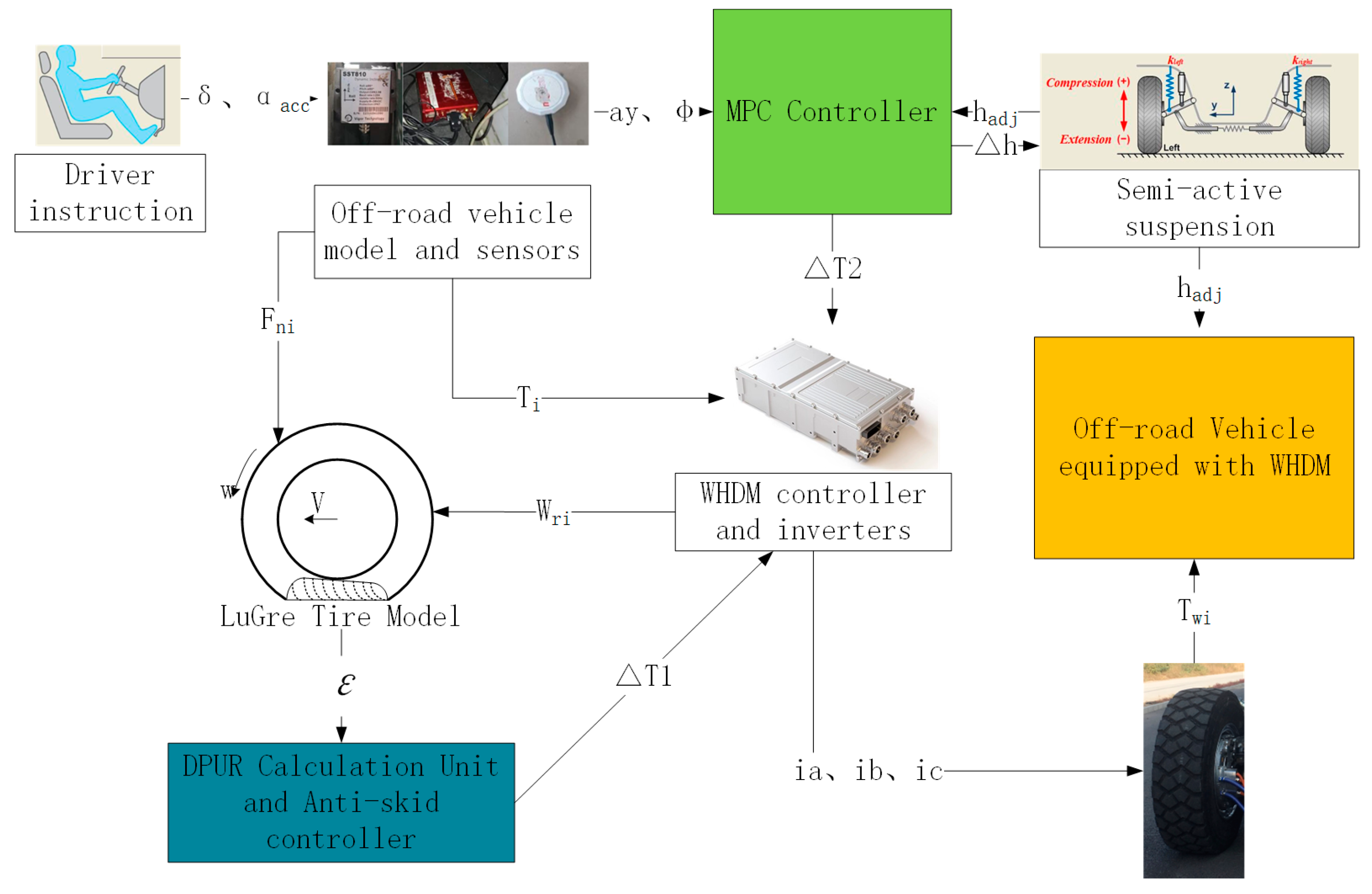
To validate the trafficability of the controlled vehicle, four experiments were designed to simulate off-road environments like steep slopes, slippery roads, slimy muddy roads and potholes. Figure 3 illustrates that a SST810 dynamic inclinometer with dynamic accuracy ±0.4% was fixed on the position of the static CG to measure the acceleration and inclination angle, and the data were optimized by a Kalman filter. The actual velocity and yaw angle were measured by a GPS.

In the first test, the vehicle climbed to the tops of the ramps at certain standard gradients (40% and 60%). Here, the two slopes’ lengths were greater than 20 m, and the change rates of the slopes conformed to the road design requirements from GB/T 12539-2018 [37]. Figure 4 shows that the test scenarios and $\mu$ of slopes were nearly equal to 0.8. $F_z$ imposed on the front and rear axles are estimated in the VCU based on the 14 DOF vehicle model, and ${\lambda }_i$ was expected to remain unanimous by adjusting the desired current of each WHDM. The significance parameters of the tested off-road vehicle and the reference values of real-vehicle test conditions were shown in

Table 2. Significance parameters of the tested off-road vehicle.

Test Conditions	Reference Value
The curb weight	$m=4800\mathrm{k}\mathrm{g}$
Speed ratio of wheel-side planetary gear reducer	$i_m=5$
Wheel base	$L=3500\mathrm{m}\mathrm{m}$
Static load ratio of the front and rear axle static load ratio	$L_f/L_r\approx 0.94$
Track width	$t_W=2100\mathrm{m}\mathrm{m}$
Effective rolling radius of tire	$r_W=425\mathrm{m}\mathrm{m}$
The wheel rotational inertial	$J_w=5\mathrm{k}\mathrm{g}·{\mathrm{m}}^2$
Maximum front wheel angle	${\delta }_{F\_\mathrm{m}\mathrm{a}\mathrm{x}}=32\mathrm{d}\mathrm{e}\mathrm{g}$
Transmission ratio of steering system	$i_s=13.6$
Minimum ground clearance	$h_{mG}=360\mathrm{m}\mathrm{m}$
Peak torque of single WHDM	$T_{\mathrm{m}\mathrm{a}\mathrm{x}}=1600\mathrm{N}\mathrm{m}$
Peak power of single WHDM	$P_{\mathrm{m}\mathrm{a}\mathrm{x}}=100\mathrm{k}\mathrm{W}$
Peak rotational speed of single WHDM	$w_{\mathrm{m}\mathrm{a}\mathrm{x}}=4800\mathrm{r}\mathrm{p}\mathrm{m}$

and

Table 3. The reference values of real-vehicle test conditions.

Test Conditions	Reference Value
Standard gradient of the first climb experiment	$I_1=40\%$
Standard gradient of the second climb experiment	$I_2=60\%$
Ramp angle of the first cross-axis test	${\theta }_{c1}=12\mathrm{d}\mathrm{e}\mathrm{g}$
Maximum vertical height of the first cross-axis test	$h_{\mathrm{m}\mathrm{a}\mathrm{x}1}=200\mathrm{m}\mathrm{m}$
Ramp angle of the second cross-axis test	${\theta }_{c2}=20\mathrm{deg}$
Maximum vertical height of the second cross-axis test	$h_{\mathrm{m}\mathrm{a}\mathrm{x}2}=400\mathrm{m}\mathrm{m}$
Adhesion coefficient of the wet basalt surface	${\mu }_{low}\approx 0.25$
Adhesion coefficient of the concrete surface	${\mu }_{high}\approx 0.9$

, respectively.

Continuous uphill cross-axis tests simulated bumpy roads or mountainous regions in which certain wheels may be easily vacated, while the other wheels would provide sufficient $F_x$ to fit the wheel resistance changing frequently and greatly. To avoid crashing the chassis, the vertical heights of the test rods were limited by $h_{mG}$. Thus, two standard twist lanes with different approach/departure angles and maximum vertical heights selected at the national automobile quality supervision and test center (NAST) were selected. Accordingly, the wavelength of these standard test roads was nearly 7 m, and the length of the straight section was 3 m. The test procedures obeyed GB/T 12541-2023 [38].

In terms of the slippery roads or muddy roads where ${\mu }_i$ were different and ${\dot{\mu }}_i$ were great, a four-wheel-drive system (4WD) was essential in ensuring that the four wheels output appropriately $F_x$ and avoid slipping. The designed ASC was expected to improve both $DPU{R}_i$ and $V_x$. As the metal surface that dripped water continuously was similar to a wet basalt surface, and since the concrete pavement possessed a high adhesion limit, three groups of experiments were designed:

(1)

$\mu$ was small: Accelerate on the slippery road;

(2)

$\dot{\mu }$ was great: Accelerate from the cement road to the slippery road;

(3)

${\mu }_i$ differed greatly: Acceleration test where the left and right wheels were on the slippery and cement road, respectively.

Three control groups were set concluding ASC for a single wheel, ASC and open differential control (ODC) for coaxial wheels and only ODC for coaxial wheels in order to appraise the performance of ASC. The velocity and stability of the controlled vehicles served as evaluation indexes. Moreover, according to the test principle, a strategy was not available if the vehicle had instability or WHDM faults occurred. The pilot always remained the same, and the number of passengers was also fixed during the tests to maintain the identical driving habit and static position of the CG.

4.1.2. Analysis of Real-Vehicle Tests

To increase the ground area and the friction force in low- velocity off-road conditions, the tire pressure should be decreased. Considering the constraint of the tire load under different pressures as well as the front axle load is less than that of the rear axle, the range of pressure adjustment should be limited to 150 kPa. To this effect, the front and rear tire pressures were decreased from the normal pressure (520 kPa) to 380 kPa and 420 kPa, respectively.

First, according to GB/T12539-2018 [37], the climbing experiment is designed to verify whether ${\lambda }_i$ can be effectively constrained by ASC intervention when the CG moves significantly backward, in which the driver should control $V_x$ close to stability and not more than 10 km/h during the test. Figure 5 shows test results of the climbing experiment with a standard gradient of 60%. The vibration in the output signal is due to the fact that the data shown are the original data that were not filtered during the test in order to reflect the true state of the vehicle. As shown in Figure 4b and Figure 5b, in the two climbing tests with design slopes I1 and I2, the ratio $F_{xFront}/F_{xRear}$ gradually decreases from 0.944 to 0.623 and 0.54. In addition, the ratio $F_{xLeft}/F_{xRight}$ is approximately 1 due to the small side slope and the lateral deviation of CG, and Vx is manually controlled in the range of 5–10 km/h. Based on the real-time calculation of (${\widehat{F}}_{zi}/mg$), the current adjustment of WHDMs makes the speed difference between the four wheels very small, as shown in Figure 4c and Figure 5c.

Table 4. The maximal slip rate and torque of four wheels during the climbing experiments.

${\mathit{\lambda }}_{\mathit{m}\mathit{a}\mathit{x}}$$\mathbf{and}{\mathit{T}}_{\mathit{w}\mathit{m}\mathit{a}\mathit{x}}$ of Four Wheels	Gradient of 40%	Gradient of 60%
${\lambda }_{maxFL}$	15.74%	19.62%
${\lambda }_{maxFR}$	15.64%	19.13%
${\lambda }_{maxRL}$	15.34%	18.63%
${\lambda }_{maxRR}$	15.15%	18.67%
$T_{wmaxFL}$	1805 Nm	2240 Nm
$T_{wmaxFR}$	1790 Nm	2250 Nm
$T_{wmaxRL}$	2580 Nm	3995 Nm
$T_{wmaxRR}$	2610 Nm	4010 Nm

and Figure 4d and Figure 5d show that the peak slip rate ${\lambda }_{maxi}$ of each wheel is less than 20%, indicating that the ASC intervention can achieve coordinated optimization of the four-wheel attachment and high margin of stability of the results of the four-wheel, similar to the simulation test, and finally reach the performance index of passing a ramp of 60% at low speed.

Figure 6a and Figure 7a demonstrate that $\varphi$, $\theta$ and $LTR$ were within controllable ranges, however, $\dot{\theta }$ and $\dot{\varphi }$ were great when $h_{zFL},h_{zFR},h_{zRL},h_{zRR}$ rapidly fluctuating during the cross-axis experiments. Hence, the presence of mutations on ${\mu }_i$ was judged. Benefiting from large inertia and long suspension travel, the suspension system effectively conducted $F_{zi}$ to the four tires and $F_{xi}$ was enough to overcome road resistance during the first cross-axis test, thus, as shown in Figure 6c, $DPU{R}_i$ is equal to 1, indicating that there is no divergence trend in the speed difference, the slip rate of each wheel. Figure 6b illustrates several $T_{wi}$ rises ($T_{wmaxi}\approx 500\mathrm{N}\mathrm{m}$) that occur within the first ten seconds of passing the first set of roadblocks, after which Twi remains near the minimum creep moment (150 Nm) and the vehicle passes the remaining roadblocks smoothly through inertia. As shown in Figure 7c, when the maximum vertical height increases to $h_{max2}$, the spring in the diagonal position is easily stretched to its limit and the corresponding $F_{zi}$ drops sharply. Since the rear of the vehicle is heavier, the CG is easily shifted to the right rear wheel or left rear wheel, so ${\dot{F}}_{zFront}$ is greater than ${\dot{F}}_{zRear}$ and the front wheel overspeed is more pronounced. The LuGre tire model detects a rapid decrease in ${\mu }_i$ and $T_{wi}$ mutations to enhance $DPU{R}_i$, or a rapid increase in response to driving intention, which is reflected in Figure 7d as an alternating sudden decrease in $DPU{R}_i$ for both sets of diagonal wheel adhesion utilization. Figure 7b shows that based on the transient rise or fall of $DPU{R}_i$ and the accurate estimation of the attachment limit of each wheel, the attachment utilization of the driving wheels can be optimized to overcome the large driving resistance, and the convergence rate of the vacated wheel slip rate is increased, which plays a role in reducing the transmission loss, and finally the performance index of continuously passing 12 large twisting roadblocks at low speed is achieved.

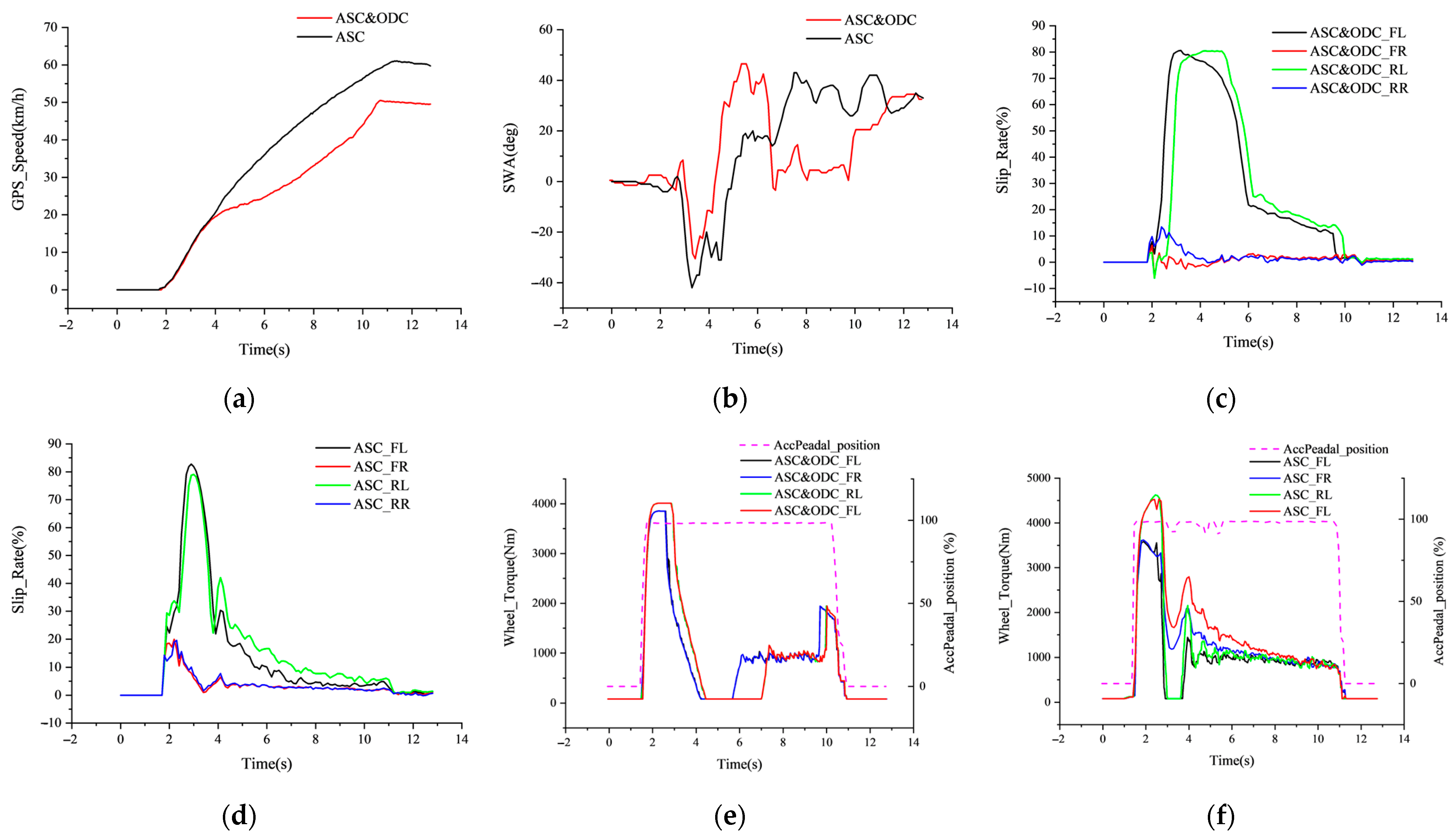
The first acceleration test simulated all four wheels being on a muddy or slippery road, so that all four wheels were all ready for overspeed. Figure 8d shows that ${\lambda }_i$ cannot be effectively suppressed under the ODC of differential speed without differential torque of the coaxial wheels, and the nonlinear decrease in the longitudinal force of the low attached wheels generates additional transverse sway moments that deteriorate the handling stability, as shown in Figure 8b, and the driver needs to apply a larger steering wheel turning angle to correct the driving trajectory; in addition, the front wheel attachment limit further decreases due to the backward shift of the droop load, making $WHD{H}_{FL}$ and $WHD{H}_{FR}$ in Figure 8f triggered the overspeed protection at 3.6 s and no more torque was output, and the same failure occurred at 9.1 s for $WHD{H}_{RL}$ and $WHD{H}_{RR}$. In contrast, Figure 8e shows that SOSMC designed in this paper is enabled at the 3.4 s and the feedforward link actively suppresses the maximum output torque T_wmax after capturing the drop in the attachment limit of each wheel, so that the four-wheel slip rate in Figure 8c drops to within 20% simultaneously in approximately 3.6 s, after which the vehicle continues to accelerate steadily. The comparison results in

Table 5. Performance comparison of controllers during the acceleration experiment on a low-adhesion road.

	Performance	${\mathit{\delta }}_{\mathbf{m}\mathbf{i}\mathbf{n}}$	${\mathit{\delta }}_{\mathbf{m}\mathbf{a}\mathbf{x}}$	$\Delta {\mathit{\delta }}_{\mathbf{m}\mathbf{a}\mathbf{x}}$	${\mathit{V}}_{\mathbf{x}\mathbf{m}\mathbf{a}\mathbf{x}}$	${\overline{\mathit{a}}}_{\mathbf{x}}$
Controllers
ODC		−104 deg	75 deg	179 deg	35.5 km/h	0.28 g
ASC AND ODC		−57 deg	39 deg	96 deg	48.9 km/h	0.098 g

show that the average vehicle acceleration is optimized by 150% and the steering wheel correction operation is relatively mild, achieving a coordinated optimization of power and stability.

When $\left|{\mu }_{Left}-{\mu }_{Right}\right|$ is large, or when only one wheel has sufficient traction, $T_w$ should be assigned more to the wheel with the larger $F_{x\max i}$, but the additional $M_z$ caused by $\left|F_{xLeft}-F_{xRight}\right|$ should be evaluated, anticipating that the ODC can partially optimize stability. In this test, vehicle stability and trafficability were compared by ASC and ASC & ODC interventions, and the need for ODC was evaluated using the comparison. Figure 9c,e show that under the control of ASC AND ODC, the left-side wheel moments $T_{wFL}$ and $T_{wRL}$ drop rapidly to within 100 Nm in 2.8 and 3 s, respectively, and correspondingly, the left-side wheel slip rates ${\lambda }_{FL}$ and ${\lambda }_{RL}$ drop from 80% to 20% in 1.5 s, and $T_{wFL}$ and $T_{wRL}$ rise rapidly and optimize acceleration after the slip rates converge, while The feedforward link limits the peak driving torque of the left low attached wheel to within 2000 Nm to avoid another longitudinal instability; in addition, the sudden increase in the left motor speed increases the power loss, which makes the right wheel torque $T_{wFR}$ and $T_{wRR}$ also decrease. Under the effect of ODC, ${\lambda }_{FL}$ and ${\lambda }_{RL}$ in Figure 9d gradually converge to the stability domain 4 s after the test starts, and the heteroside wheel torque difference is always zero, as shown in Figure 9f, which lowers the utilization of high attached wheel adhesion on the right and the average vehicle acceleration decreases by 23% compared to the ASC AND ODC control group. In terms of lateral stability, as shown in Figure 9b, although the driver was forced to correct the driving trajectory due to the large transverse sway motion in the first part of acceleration, the real-time differential torque control of each wheel through ASC AND ODC improved the stability margin of each wheel in time and effectively avoided the loss of steering control caused by the nonlinear decrease in wheel lateral deflection stiffness. The comparison results in

Table 6. Performance comparison of controllers during the acceleration experiment on a split road.

	Performance	${\mathit{\delta }}_{\mathit{m}\mathit{i}\mathit{n}}$	${\mathit{\delta }}_{\mathit{m}\mathit{a}\mathit{x}}$	$\Delta {\mathit{\delta }}_{\mathit{m}\mathit{a}\mathit{x}}$	${\mathit{V}}_{\mathit{x}\mathit{m}\mathit{a}\mathit{x}}$	${\overline{\mathit{a}}}_{\mathit{x}}$
Controllers
ODC		−42 deg	43 deg	85 deg	61.1 km/h	0.18 g
ASC AND ODC		−31 deg	47 deg	78 deg	50.5 km/h	0.14 g

show that the deviation between the steering wheel angles in the two sets of tests is less than 10% and the peak value does not exceed 47 deg, indicating that the additional transverse moment is small and always within the controllable range.

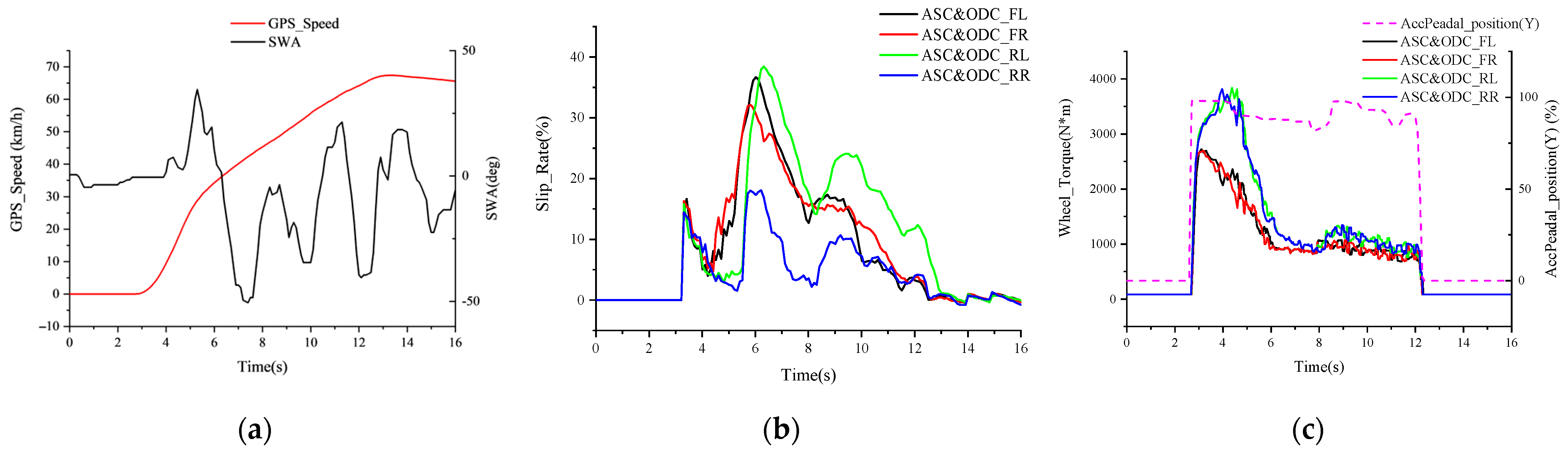
The docking road acceleration test can further verify the robustness of the ASC AND ODC distribution strategy in the face of transient perturbations. As shown in Figure 10b,c, with the rapid increase in wheel-end drive torque, the slip rate ${\lambda }_i$ reaches 16% at 3.5 s and does not disperse significantly due to the high adhesion limit, while the front and rear wheels enter the low-adhesion road at 4.5 and 5.6 s, respectively, and their slip rate rises abruptly afterwards, and the estimated adhesion coefficients of the front and rear wheels decrease rapidly, and the maximum output torque of a single wheel is limited actively in the feedforward link $T_{w\max }$ and the combined effect of longitudinal stability feedback control, the front and rear wheel slip rates start to converge at 5.5 and 6 s, respectively, and the response delay of ASC AND ODC is less than 0.5 s; after 6 s, ASC AND ODC takes the optimization goal of improving the adhesion utilization rate of each wheel, so that $T_{wi}\approx r_w{F}_{xmaxi}$, and carries out a continuous and stable approximate uniform acceleration motion as shown in Figure 10a, as in

Table 7. Performance of the controller ASC AND ODC during the acceleration experiment on a road with great $\dot{\mu }$.

	Performance	${\mathit{\delta }}_{\mathit{m}\mathit{i}\mathit{n}}$	${\mathit{\delta }}_{\mathit{m}\mathit{a}\mathit{x}}$	$\Delta {\mathit{\delta }}_{\mathit{m}\mathit{a}\mathit{x}}$	${\mathit{V}}_{\mathit{x}\mathit{m}\mathit{a}\mathit{x}}$	${\overline{\mathit{a}}}_{\mathit{x}}$
Controllers
ASC AND ODC		−50 deg	34 deg	84 deg	67.5 km/h	0.203 g

exceeds 0.2 g, considering that the road adhesion coefficient is in the range [0.2, 0.25], indicating that the average drive power utilization exceeds 80% and max does not exceed 50 deg, achieving a coordinated optimization of dynamics and longitudinal and transverse stability.

According to the above analysis, ${\widehat{F}}_{zi}$ and ${\widehat{\mu }}_i$ can be updated by the vehicle dynamic model and the LuGre tire model, respectively, in VCU. Therefore, the utilization of ${\mu }_i$ can be maintained as consistently as possible, and ASC can suppress ${\lambda }_i$ with a slight lag. However, the ODC was found to be indispensable in ensuring lateral stability, and $a_x$ can be forced to be reduced if ${\mu }_i$ abruptly changes with a great $V_x$.

4.2. HIL Simulation

4.2.1. Simulation Environment

The dSPACE hardware-in-the-loop (HIL) simulation platform primarily consists of an upper host computer and a lower-level control unit cabinet. The lower-level control unit cabinet can be further divided into the MicroAutoBox II (rapid prototyping controller) and SCALEXIO (real-time simulator). The MicroAutoBox II and SCALEXIO are, respectively, utilized for real-time execution of control strategies and simulating a “human–vehicle–road” closed-loop environment. SCALEXIO incorporates whole vehicle models and road environment models, while MicroAutoBox II leverages the CAN communication and analog-digital conversion modules built into Simulink to acquire feedback on vehicle state parameters calculated by the integrated models within SCALEXIO. The HPS model was established in the MATLAB/Simulink (R2017b) software, and the side slope passing test and the sine wave steering test on roads with different $\mu$ were designed in order to verify the rollover prevention effect of MPC. The first test simulated conditions where the roll moment was mainly decided by the obvious difference between $h_{zLeft}$ and $h_{zRight}$. Here, $a_y$ is usually small since the pilot should maintain a low $V_x$ to acquire sufficiently $F_y$ and overcome side slope resistance. Thus, the desired $V_x$ was set as 10 km/h. Since $L\dot{T}R$ was modest, $h_s$ was expected to gradually descend to a suitable value adjusted by the models of MPC and HPS.

The great ${\dot{F}}_{yi}$ readily occur under certain violent turning operations on flat roads, hence $LTR$ should be promptly predicted while the desired $h_s$ could rapidly decrease. Furthermore, the angle of slipping of the tires was rather large on roads with low-adhesion roads, and $a_y$ was relatively smaller since $F_{ymaxi}$ was restricted by the appearance of an adhesion limit, resulting in the tracking error. The desired SWA is expressed in Figure 11a, while the desired $V_x$ was equal at 60 km/h and $\mu$ was set to 0.85 and 0.25, respectively. The HIL test environment as shown in Figure 11b.

4.2.2. Comparative Validation

Expressed as the red line in Figure 12a, the value of $\left(h_s\ast cos\varphi \right)$ decreased from 0.97 m to 0.8 m with the improvement in a slant angle, while the roll arm was significantly descended by MPC and HPS. The black line in Figure 12a shows that $\Delta h_s$ dropped rapidly before the 4th second as $L\tilde{T}R$ and $L\dot{\tilde{T}}R$ improved while the road began to tilt. Afterward, $\Delta h_s$ changed slowly since $L\dot{\tilde{T}}R$ was timely restrained, and $\left(h_s\ast cos\varphi \right)$ reduced to 0.42 m after the 14th second. Consequently, $LTR$ reduced from 0.61 to 0.38, and $F_{yLeft}$ increased by 55% since the improvement of the left wheels’ vertical load with the control of MPC when the vehicle continued to run on the 30 deg slant slope, as shown in Figure 12b,c. According to the comparative analysis, the roll stability can be effectively improved by the designed MPC at the functional level.

When performing the violent turning motion on the higher adhesion road, the tires’ cornering stiffness was large enough to generate sufficient $F_y$ with a smaller slip angle. To this effect, the response of steering instructions improved; however, the roll moment created by $a_y$ was greater along with the rollover risk $(\left|LT{R}_{max}\right|>0.8)$, depicted by the blue lines in Figure 13b. In addition, Figure 13a expounded that $h_s$ was decreased by 0.32 m under the adjustment of MPC since $a_y$ and $\left|L\tilde{T}R\right|$ sharply increased while SWA began to mutate. In contrast, the model of HPS had a response delay in which the desired $h_s$ was achieved prior to the 5th second, after which $\left|L\tilde{T}R\right|$ and $\Delta h_s$ gradually converged to zero while $\left|LT{R}_{max}\right|$ was limited to 0.4 or less, as demonstrated by the green lines in Figure 13b. Meanwhile, $\left|{\mathsf{\beta }}_{max}\right|$ decreased from 2.4 deg to 1.2 deg, as shown in Figure 13c. Thus, the tracking error had a decline of 50%.

When the tire makes a violent turning movement on a low-adhesion road, the turning stiffness of the tire is relatively small, and a larger slip angle will occur, generating less lateral force and less risk of rollover. When $\mu$ decreased, $F_{ymaxi}$, $a_y$ and roll moment all reduced significantly. As shown in Figure 14a, when the road adhesion coefficient decreases, $\left(h_s\ast cos\varphi \right)$ starts to drop from the 7th second due to the intervention of MPC control, and tends to stabilize and remain at 0.63 m after 25 s, a drop of 0.34 m. As shown in Figure 14b, $\left|LT{R}_{max}\right|$ does not exceed 0.35. Figure 14c shows that the decreased $h_s$ could not effectively restrain the tracking error under the transient steering operation with a low $\mu$.

5. Conclusions

This paper innovatively proposes an effective anti-skid control method with superior real-time robustness, combined with a rollover algorithm to comprehensively consider the passing performance and stability of off-road vehicles, specifically including

(1)

To adapt to the strong interference of different tires on unpaved roads, an attachment state monitor consisting of a LuGre tire model, a resolver and an inertial sensor is proposed, in which ASC is used to improve the adhesion condition based on a 4 WHDM drive power utilization rate (DPUR) to achieve fast and smooth convergence of the slip rate under off-road conditions.

(2)

A nonlinear 14 DOF vehicle model is developed to estimate LTR in MPC for a limited time range to avoid rollover in advance by adjusting the SAS model.

(3)

During the experiments, the designed ASC maintains the drive-power utilization rate ($DPU{R}_i$) around 0.9 after the unloaded wheels of the designed ASC enter the surface of the slip model and their convergence time is reduced to 100 ms.

(4)

The designed MPC outputs the amount of suspension height adjustment at the appropriate adjustment rate, thus adjusting the lateral load transfer ratio error change rate ($L\dot{\tilde{T}}R$) and the lateral load transfer ratio maximum ($LT{R}_{max}$).

(5)

Furthermore, the feasibility of anti-rollover was verified on the HIL platform through sharp curves or violent steering on different roads.

References

1. Sun, X.; Wang, Y.; Cai, Y.; Wong, P.K.; Chen, L.; Bei, S. Nonsingular terminal sliding mode based direct yaw moment control for four-wheel independently actuated autonomous vehicles. IEEE Trans. Transp. Electrif. 2023, 9, 2568–2582. [Google Scholar] [CrossRef]
2. Huang, C.; Wu, X.; Wu, C.; Wang, J.; Shu, X. Rule-based torque vectoring distribution strategy combined with slip ratio control to improve the handling stability of distributed drive electric vehicles. Proc. Inst. Mech. Eng. Part D J. Automob. Eng. 2024. [Google Scholar] [CrossRef]
3. Wang, Y.; Kang, F.; Wang, T.; Ren, H. A robust control method for lateral stability control of in-wheel motored electric vehicle based on sideslip angle observer. Shock. Vib. 2018, 2018, 8197941. [Google Scholar] [CrossRef]
4. Ma, L.; Cheng, C.; Guo, J.; Shi, B.; Ding, S.; Mei, K. Direct yaw-moment control of electric vehicles based on adaptive sliding mode. Math. Biosci. Eng. 2023, 20, 13334–13355. [Google Scholar] [CrossRef] [PubMed]
5. Park, J.; Jang, I.G.; Hwang, S.-H. Torque distribution algorithm for an independently driven electric vehicle using a fuzzy control method: Driving stability and efficiency. Energies 2018, 11, 3479. [Google Scholar] [CrossRef]
6. Ge, P.; Guo, L.; Feng, J.; Zhou, X. Adaptive Stability Control Based on Sliding Model Control for BEVs Driven by In-Wheel Motors. Sustainability 2023, 15, 8660. [Google Scholar] [CrossRef]
7. Kim, H.S.; Hyun, Y.J.; Nam, K.H. Disturbance observer-based sideslip angle control for improving cornering characteristics of in-wheel motor electric vehicles. Int. J. Automot. Technol. 2018, 19, 1071–1080. [Google Scholar] [CrossRef]
8. Hassan, A.; Frejo, J.R.D.; Maestre, J.M. An Assessment of Predictive Control Strategies for Lateral Stability Control of 4-Wheels Drive Electrical Vehicle. In Proceedings of the 2023 8th International Conference on Control and Robotics Engineering (ICCRE), Niigata, Japan, 21–23 April 2023; pp. 177–182. [Google Scholar]
9. Guo, N.; Zhang, X.; Zou, Y. Real-time predictive control of path following to stabilize autonomous electric vehicles under extreme drive conditions. Automot. Innov. 2022, 5, 453–470. [Google Scholar] [CrossRef]
10. Wei, L.; Wang, X.; Li, L.; Fan, Z.; Dou, R.; Lin, J. TS fuzzy model predictive control for vehicle yaw stability in nonlinear region. IEEE Trans. Veh. Technol. 2021, 70, 7536–7546. [Google Scholar] [CrossRef]
11. Aksjonov, A.; Vodovozov, V.; Augsburg, K.; Petlenkov, E. Design of regenerative anti-lock braking system controller for 4 in-wheel-motor drive electric vehicle with road surface estimation. Int. J. Automot. Technol. 2018, 19, 727–742. [Google Scholar] [CrossRef]
12. Yoon, J.-H.; Eben Li, S.; Ahn, C. Estimation of vehicle sideslip angle and tire-road friction coefficient based on magnetometer with GPS. Int. J. Automot. Technol. 2016, 17, 427–435. [Google Scholar] [CrossRef]
13. Liu, J.; Liu, H.; Wang, J.; Gu, H. Coordinated Lateral Stability Control of Autonomous Vehicles Based on State Estimation and Path Tracking. Machines 2023, 11, 328. [Google Scholar] [CrossRef]
14. Canudas-De-Wit, C.; Horowitz, R. Observers for tire/road contact friction using only wheel angular velocity information. In Proceedings of the 38th IEEE Conference on Decision and Control (Cat. No. 99CH36304), Phoenix, AZ, USA, 7–10 December 1999; pp. 3932–3937. [Google Scholar]
15. Matsuzaki, R.; Kamai, K.; Seki, R. Intelligent tires for identifying coefficient of friction of tire/road contact surfaces. In Proceedings of the Sensors and Smart Structures Technologies for Civil, Mechanical, and Aerospace Systems 2015, San Diego, CA, USA, 9–12 March 2015; pp. 84–92. [Google Scholar]
16. Singh, K.B.; Taheri, S. Estimation of tire–road friction coefficient and its application in chassis control systems. Syst. Sci. Control Eng. 2015, 3, 39–61. [Google Scholar] [CrossRef]
17. Jin, L.-Q.; Ling, M.; Yue, W. Tire-road friction estimation and traction control strategy for motorized electric vehicle. PLoS ONE 2017, 12, e0179526. [Google Scholar] [CrossRef]
18. Kanungo, A.; Kumar, P.; Gupta, V.; Saxena, N.K. A design an optimized fuzzy adaptive proportional-integral-derivative controller for anti-lock braking systems. Eng. Appl. Artif. Intell. 2024, 133, 108556. [Google Scholar] [CrossRef]
19. Liu, S.T.; Chang, C.W.; Huang, Y.H.; Lin, T.H.; Chiu, J.; Lee, J.L. Development and Test of ABS/TCS Controller with Dual-Axis Dynamometer HIL Platform; SAE Technical Paper; SAE International: Warrendale, PA, USA, 2023. [Google Scholar]
20. El-bakkouri, J.; Ouadi, H.; Saad, A. Adaptive neuro fuzzy inference system based controller for electric vehicle’s hybrid ABS braking. IFAC-PapersOnLine 2022, 55, 371–376. [Google Scholar] [CrossRef]
21. Wu, J.; Zhao, Y.; Ji, X.; Liu, Y.; Zhang, L. Generalized internal model robust control for active front steering intervention. Chin. J. Mech. Eng. 2015, 28, 285–293. [Google Scholar] [CrossRef]
22. Ghazali, M.; Durali, M.; Salarieh, H. Vehicle trajectory challenge in predictive active steering rollover prevention. Int. J. Automot. Technol. 2017, 18, 511–521. [Google Scholar] [CrossRef]
23. Chen, C.; Zhang, G.; Qian, Z.; Tarefder, R.A.; Tian, Z. Investigating driver injury severity patterns in rollover crashes using support vector machine models. Accid. Anal. Prev. 2016, 90, 128–139. [Google Scholar] [CrossRef] [PubMed]
24. Islam, S.; Hossain, A.B.; Barnett, T.E. Comprehensive injury severity analysis of SUV and pickup truck rollover crashes: Alabama case study. Transp. Res. Rec. 2016, 2601, 1–9. [Google Scholar] [CrossRef]
25. Nguyen, T.A. Establishing a novel adaptive fuzzy control algorithm for an active stabilizer bar with complex automotive dynamics model. Ain Shams Eng. J. 2024, 15, 102334. [Google Scholar] [CrossRef]
26. Nguyen, T.A.; Iqbal, J.; Tran, T.T.H.; Hoang, T.B. Application of hybrid control algorithm on the vehicle active suspension system to reduce vibrations. Adv. Mech. Eng. 2024, 16, 16878132241239816. [Google Scholar] [CrossRef]
27. Li, H.; Zhao, Y.; Lin, F.; Zhu, M. Nonlinear dynamics modeling and rollover control of an off-road vehicle with mechanical elastic wheel. J. Braz. Soc. Mech. Sci. Eng. 2018, 40, 51. [Google Scholar] [CrossRef]
28. Wnag, C.; Zhao, W.; Xu, Z.; Zhou, G. Path planning and stability control of collision avoidance system based on active front steering. Sci. China Technol. Sci. 2017, 60, 1231–1243. [Google Scholar] [CrossRef]
29. Chen, Z.; Wu, Y.; Li, F. Integrated control of differential braking and active aerodynamic control for improving high speed stability of vehicles. Int. J. Automot. Technol. 2020, 21, 61–70. [Google Scholar] [CrossRef]
30. Her, H.; Suh, J.; Yi, K. Integrated control of the differential braking, the suspension damping force and the active roll moment for improvement in the agility and the stability. Proc. Inst. Mech. Eng. Part D J. Automob. Eng. 2015, 229, 1145–1157. [Google Scholar] [CrossRef]
31. Nguyen, T.A. Development of a Novel Integrated Control Strategy for Automotive Electric Power Steering Systems. IEEE Trans. Autom. Sci. Eng. 2024. [Google Scholar] [CrossRef]
32. Zhang, L.; Li, L.; Qi, B. Rollover prevention control for a four in-wheel motors drive electric vehicle on an uneven road. Sci. China Technol. Sci. 2018, 61, 934–948. [Google Scholar] [CrossRef]
33. Li, L.; Lu, Y.; Wang, R.; Chen, J. A three-dimensional dynamics control framework of vehicle lateral stability and rollover prevention via active braking with MPC. IEEE Trans. Ind. Electron. 2016, 64, 3389–3401. [Google Scholar] [CrossRef]
34. Liu, J.; Gao, L.; Zhang, J.; Yan, F. Super-twisting algorithm second-order sliding mode control for collision avoidance system based on active front steering and direct yaw moment control. Proc. Inst. Mech. Eng. Part D J. Automob. Eng. 2021, 235, 43–54. [Google Scholar] [CrossRef]
35. Xu, G.; Xu, K.; Zheng, C.; Zahid, T. Optimal operation point detection based on force transmitting behavior for wheel slip prevention of electric vehicles. IEEE Trans. Intell. Transp. Syst. 2015, 17, 481–490. [Google Scholar] [CrossRef]
36. Aligia, D.A.; Magallan, G.A.; De Angelo, C.H. EV traction control based on nonlinear observers considering longitudinal and lateral tire forces. IEEE Trans. Intell. Transp. Syst. 2017, 19, 2558–2571. [Google Scholar] [CrossRef]
37. GB/T 12541-2023; Motor Vehicles Passing Capacity Test Method. State Administration for Market Regulation, National Standardization Management Committee: Beijing, China, 2023.
38. GB/T 12539-2018; Motor Vehicles Steep Hill Climbing Test Method. State Administration for Market Regulation, National Standardization Management Committee: Beijing, China, 2018.
Figure 1. Nonlinear 14 DOF vehicle dynamic model. (a) Dynamic model of the vehicle in the XY plane. (b) Dynamic model of the vehicle in the YZ plane. (c) Dynamic model of the vehicle X-Z plane.
Mathematics 12 01871 g001
Figure 2. Logic diagram of the vehicle stability control module.
Mathematics 12 01871 g002
Figure 3. Sensor systems of real-vehicle experiments.
Mathematics 12 01871 g003
Figure 4. Results of the real-vehicle test of the climbing experiment with a standard gradient of 40%. (a) Pitch and roll angles of the carriage. (b) Output torques of the four wheels. (c) Rotation speeds of the four wheels. (d) Slip rates of the four wheels.
Mathematics 12 01871 g004
Figure 5. Test results of the climbing experiment with a standard gradient of 60%. (a) Pitch and roll angles of the carriage. (b) Output torques of the four wheels. (c) Rotation speeds of the four wheels. (d) Slip rates of the four wheels.
Mathematics 12 01871 g005
Figure 6. Results of cross-axis experiment with the maximum vertical height h m a x 1 . (a) Pitch and Roll angles of the carriage. (b) Output torques of the four wheels. (c) Rotation speeds of the four wheels.
Mathematics 12 01871 g006
Figure 7. Results of cross-axis experiment with the maximum vertical height h m a x 2 . (a) Pitch and Roll angles of the carriage. (b) Output torques of the four wheels. (c) Rotation speeds of the four wheels. (d) DPUR of the four wheels.
Mathematics 12 01871 g007
Figure 8. Results of the acceleration experiment on a low-adhesion road ( μ μ L o w ). (a) The measured vehicle velocity under different controllers. (b) SWA under different controllers. (c) Slip rates of the four wheels under the controller ASC AND ODC. (d) Slip rates of the four wheels under the controller ODC. (e) Output torques of the four wheels response to the accelerating demand under the controller ASC AND ODC. (f) Output torques of the response of the four wheels’ response to the accelerating demand under the ODC controller.
Mathematics 12 01871 g008
Figure 9. Results of the acceleration experiment on a split road ( μ L e f t μ L o w , μ R i g h t μ h i g h ). (a) The vehicle velocity under different controllers. (b) SWA under different controllers. (c) Slip rates of the four wheels under the controller ASC AND ODC. (d) Slip rates of the four wheels under the controller ASC. (e) Output torques of the four wheels response to the accelerating demand under the controller ASC AND ODC. (f) Output torques of the response of the four wheels’ response to the accelerating demand under the ASC controller.
Mathematics 12 01871 g009
Figure 10. Results of the acceleration experiment on a road with great μ ˙ ( μ h i g h μ L o w ). (a) The measured vehicle velocity and SWA under the controller ASC AND ODC. (b) Slip rates of the four wheels under the controller ASC AND ODC. (c) Output torques of the four wheels response to the accelerating demand under the controller ASC AND ODC.
Mathematics 12 01871 g010
Figure 11. The simulation environment setting. (a) The desired SWA. (b) The HIL test environment.
Mathematics 12 01871 g011
Figure 12. Performance validation of the controller MPC through the side slope passing simulation test. (a) The curve of roll arm’s length with the control of MPC or not. (b) The curve of LTR with the control of MPC or not. (c) The curve of the left wheels’ lateral force with the control of MPC or not.
Mathematics 12 01871 g012
Figure 13. Performance validation of the controller MPC through the sine wave steering simulation test ( μ = 0.85 ). (a) The curve of roll arm’s length with the control of MPC or not. (b) The curve of LTR with the control of MPC or not. (c) The curve of the sideslip angle with the control of MPC or not.
Mathematics 12 01871 g013
Figure 14. Performance validation of the controller MPC through the sine wave steering simulation test ( μ = 0.25 ). (a) The curve of roll arm’s length with the control of MPC or not. (b) The curve of LTR with the control of MPC or not. (c) The curve of the sideslip angle with the control of MPC or not.
Mathematics 12 01871 g014