Numerical Resolution of Differential Equations Using the Finite Difference Method in the Real and Complex Domain

Abstract

The paper expands the finite difference method to the complex plane, and thus obtains an improvement in the resolution of differential equations with an increase in numerical precision and a generalization in the mathematical modeling of problems. The article begins with a selection of the best techniques for obtaining finite difference coefficients for approximating derivatives in the real domain. Then, the calculation is expanded to the complex domain. The research expands forward, backward, and central difference approximations of the real case by a quadrant approximation in the complex plane, which facilitates the use in boundary conditions of differential equations. The article shows many real and complex finite difference equations with their respective order of error, intended to serve as a basis and reference, which have been tested in practical examples of solving differential equations used in engineering. Finally, a comparison is made between the real and complex techniques of finite difference methods applied in the Theory of Elasticity. As a surprising result, the article shows that the finite difference method has great advantages in numerical precision, diversity of formulas, and modeling generalities in the complex domain when compared to the real domain.

1. Introduction

The finite difference method can be employed to solve boundary value or initial value problems involving ordinary or partial differential equations. Thus, this method can be applied to solve the equations of models using concentrated or distributed parameters [1,2,3]. The technique consists of replacing each derivative or differential of the differential equations by approximation of finite differences or finite addition of the variables, as shown in Equation (1) below:

$$\left\{\begin{array}{c}dx\cong ∆x, dy\cong ∆y, du\cong ∆u\\ \frac{dy}{dx}\cong \frac{∆y}{∆x}\cong \frac{\nabla y}{\nabla x}\cong \frac{\delta y}{\delta x}\cong \frac{\mu \delta y}{\mu \delta x}, \frac{d^{2}y}{d{x}^2}\cong \frac{{∆}^{2}y}{∆x^2}\cong \frac{{\nabla }^{2}y}{\nabla x^2}\cong \frac{{\delta }^{2}y}{\delta x^2}, \frac{d^{3}y}{d{x}^3}\cong \frac{{∆}^{3}y}{∆x^3}\cong \frac{{\nabla }^{3}y}{\nabla x^3}\cong \frac{{\mu \delta }^{3}y}{\delta x^3}\cong \frac{{\mu \delta }^{3}y}{\mu \delta x^3} \\ \frac{\partial u}{\partial x}\cong \frac{∆u}{∆x}\cong \frac{\nabla \mathrm{u}}{\nabla x}\cong \frac{\delta u}{\delta x}\cong \frac{\mu \delta u}{\mu \delta x}, \frac{{\partial }^{2}u}{\partial x^2}\cong \frac{{∆}^{2}u}{∆x^2}, \frac{{\partial }^{3}u}{\partial x^3}\cong \frac{{∆}^{3}u}{∆x^3}, \frac{{\partial }^{2}u}{\partial x\partial y}\cong \frac{{∆}^{2}u}{\partial x\partial y}, \frac{{\partial }^{3}u}{\partial x\partial y}\cong \frac{{∆}^{3}u}{\partial x^2\partial y} \end{array}\right.$$

(1)

The error is the difference in the absolute value of the exact value and of the approximate value (Error = |Value_exact—Value_approx|). In principle, shortening the calculation step reduces the number of errors. The ratio of step to error decrease is the order of error (n), indicated by O(hⁿ), where h = Δx = x_i+1−x_i is the constant step of the independent variables [1,4]. Thus, if a numerical method is of error order O(h⁴), it means that if you shorten the step by half, the error decreases (1/2)⁴ = 1/16; that is, the error decreases approximately 16 times. If you reduce the step by 10 times, the error drops 10⁴ = 10,000 times. Therefore, the higher the error order of a method is, the more accurate the method. Most numerical methods contain errors; that is, they are approximate methods. The interesting question is to be able to reduce these errors to a level that meets the demand of the problem under investigation. Thus, this approach makes the method as accurate as one wishes [5].

The idea of replacing differentials with finite additions is derived from the origin of differential and integral calculus, where at the time of its creation, the idea of limit was not very developed. Thus, mathematicians approximated the differentials by very small positive values near zero. Therefore, the finite difference method is very simple and intuitive mathematics.

In recent years, the finite difference method has been losing ground to other numerical methods, such as the finite element method and the boundary element method. It is believed that one of the reasons for this trend is the difficulty of obtaining approximations of the derivatives by finite difference equations, especially for high-order derivatives with several variables, and finite difference formulas that have a high order of error. The present work attempts to correct this gap and starts with a review of numerical finite difference operators.

2. Review of Numerical Finite Difference Operators

The operator is a symbol that represents, in short, a set of operations to be performed on a variable [1]. The domain or field of definition of an operator is the set, to which the operator can be applied [6]. Numeric operators have as an operand or domain the images of a discrete (or tabulated) function, because numerical methods work mainly with tables of points rather than algebraic or analytic functions [4]. A discrete function (tabulated function) will be represented by the set of points {(x₁, y₁), (x₂, y₂), …, (x_n, y_n)} or {[x₁, u(x₁)], [x₂, u(x₂)], …, [x_n, u(x_n)]}, where y_n= u(x_n), and h = Δx = x_i+1-x_i is a constant step of the independent variables (h = Δx = x₂ − x₁ = x₃ − x₂ = x₄ − x₃ = x_i+1 − x_i = … = x_n − x_n−1).

Table 1. Definition of numeric operators.

Operator	Symbol	Definition
Shift	E	Eu(xi) = u(xi+1) or Eyi = yi+1
Forward difference	Δ	Δu(xi) = u(xi+1) − u(xi) or Δyi = yi+1 − yi or Δ = E − 1
Backward difference	∇	∇u(xi) = u(xi) − u(xi−1) or ∇yi = yi − yi−1 or ∇ = 1 − E−1
Central difference	δ	δu(xi) = u(xi+½) − u(xi−½) or δyi = yi+½ − yi−½ or δ = E1/2 − E−1/2
Average	μ	μu(xi) = (½)[ u(xi+½) + u(xi−½) ] or μyi = (½)(yi+½ + yi−½ ) or μ = (½)(E½ + E−½ )
Average central difference	μδ	μδu(xi) = (½)[ u(xi+1) − u(xi−1) ] or μδyi = (½)(yi+1 − yi−1) or μδ = (½)(E1 − E−1)

defines the main numeric operators.

In addition, the differential operator is usually denoted by D (the differential operator (D) is not a numeric operator), where $Df\left(x\right)=\frac{d}{dx}f\left(x\right)=f’\left(x\right) or D^{2}f\left(x\right)=\frac{d^2}{{dx}^2}f\left(x\right)=f´´\left(x\right) or D^{3}f\left(x\right)=\frac{d^3}{{dx}^3}f\left(x\right)=f´´´\left(x\right) or D^{4}f\left(x\right)=\frac{d^4}{{dx}^4}f\left(x\right)=f^{\left(4\right)}\left(x\right) or\dots or D^{n}f\left(x\right)=\frac{d^n}{{dx}^n}f\left(x\right)=f^{\left(n\right)}\left(x\right)$. Additionally, as the spacing of the variable x is constant, h = Δx = ∇x = δx = μδ x.

The numerical operators can be successively applied, which is referred to as the potence of operators, analogous to the operation of algebraic potentiation.

Table 2. Successive application of numeric operators (potentiation).

Operator	Symbol	Successive Application
Shift	E	Enu(xi) = u(xi+n) or Enyi = yi+n or En = E(E(E(….E)))
Forward difference	Δ	Δnu(xi) = Δn−1u(xi+1) − Δn−1u(xi) or Δnyi = Δn−1yi+1 − Δn−1yi or Δn = Δ(Δ(Δ(….Δ)))
Backward difference	∇	∇nu(xi) = ∇n−1u(xi) − ∇n−1u(xi−1) or ∇nyi = ∇n−1yi − ∇n−1yi−1 or ∇n = ∇(∇(∇(….∇)))
Central difference	δ	δnu(xi) = δn−1u(xi+½) − δn−1u(xi−½) or δnyi = δn−1yi+½ − δn−1yi−½ or δ n = δ(δ(δ(….δ))) δ2u(xi) = δu(xi+½) − δu(xi−½) = [u(xi+½+½) − u(xi+½−½)] − [u(xi−½+½) − u(xi−½−½)] = [u(xi+1) − u(xi)] − [u(xi) − u(xi−1)] = u(xi+1) − u(xi) − u(xi) + u(xi−1) = u(xi+1) − 2 u(xi) + u(xi−1) δ2u(xi) = u(xi+1) − 2 u(xi) + u(xi−1) or δ2yi = yi+1 − 2 yi + yi−1 δ4u(xi) = δ2u(xi+1) − 2 δ2u(xi) + δ2u(xi−1) or δ2yi = δ2yi+1 − 2 δ2yi + δ2yi−1 δnu(xi) = δn−2u(xi+1) − 2δn−2u(xi) + δn−2u(xi−1) or δnyi = δn−2yi+1 − 2δn−2yi + δn−2yi−1
Average central difference	μδ	μδnu(xi) = (½) [δn−1u(xi+½) − δn−1u(xi−½)] or μδnyi = (½) (δn−1yi+½ − δn−1yi−½ ) or μδn = μδ(δ(δ(….δ))) μδu(xi) = (½) [u(xi+1) − u(xi−1) ] or μδyi = (½)(yi+1 − yi−1) μδ3u(xi) = (½) [δ2u(xi+1) − δ2u(xi−1)] or μδ3yi = (½)(δ2yi+1 − δ2yi−1) μδnu(xi) = (½) [ δn−1u(xi+1) − δn−1u(xi−1)] or μδnyi = (½)(δn−1yi+1 − δn−1yi−1)

shows the successive application of the numeric operators, where n is any number.

3. Review of Finite Difference Equations for Derivative Approximations of a Single Variable

Finite difference equations are used to approximate derivatives of any order at any point, as long as there is a sufficient number of points [2,7,8,9,10]. To calculate the numerical value of a derivative, finite differences use nearby points and their locations. The locations of these sampled points receive the name of finite difference stencil.

To determine the coefficients for a difference equation:

$$\frac{d^{4}u}{d{x}^4}\approx Au\left(x-2h\right)+Bu\left(x-h\right)+Cu\left(x\right)+Du\left(x+h\right)+Eu(x+2h)$$

(2)

The formula for Taylor expansion is:

$$u\left(b\right)=u\left(a\right)+\frac{u´\left(a\right)}{1!}\left(b-a\right)+\frac{u´´\left(a\right)}{2!}{(b-a)}^2+\cdots +\frac{u^{\left(n\right)}\left(a\right)}{n!}{\left(b-a\right)}^n+\cdots$$

(3)

By expanding the first term, A of u(x − 2h), with b = x − 2h and a = x, we obtain:

$$\begin{array}{c}Au\left(x\right)+Au´\left(x\right)\left(-2h\right)+A\frac{1}{2}u´´\left(x\right){\left(-2h\right)}^2+A\frac{1}{6}u´´´\left(x\right){\left(-2h\right)}^3+\\ A\frac{1}{24}u´´´´\left(x\right){\left(-2h\right)}^4+A\frac{1}{120}u´´´´´\left(x\right){\left(-2h\right)}^5+\cdots \end{array}$$

(4)

We then did the same for all the other terms in the numerator:

$$\begin{array}{c}+Bu\left(x\right)+Bu´\left(x\right)\left(-h\right)+B\frac{1}{2}u´´\left(x\right){\left(-h\right)}^2+B\frac{1}{6}u´´´\left(x\right){\left(-h\right)}^3\hfill \\ +B\frac{1}{24}u´´´´\left(x\right){\left(-h\right)}^4+B\frac{1}{120}u´´´´´\left(x\right){\left(-h\right)}^5+\dots \hfill \\ +Cu\left(x\right)\hfill \\ +Du\left(x\right)+Du´\left(x\right)\left(h\right)+D\frac{1}{2}u´´\left(x\right){\left(h\right)}^2+D\frac{1}{6}u´´´\left(x\right){\left(h\right)}^3\hfill \\ +D\frac{1}{24}u´´´´\left(x\right){\left(h\right)}^4+D\frac{1}{120}u´´´´´\left(x\right){\left(h\right)}^5+\hfill \\ +Eu\left(x\right)+Eu´\left(x\right)\left(2h\right)+E\frac{1}{2}u´´\left(x\right){\left(2h\right)}^2+E\frac{1}{6}u´´´\left(x\right){\left(2h\right)}^3\hfill \\ +E\frac{1}{24}u´´´´\left(x\right){\left(2h\right)}^4+E\frac{1}{120}u´´´´´\left(x\right){\left(2h\right)}^5+\cdots \hfill \end{array}$$

(5)

Now, to choose A, B, C, D, and E such that the summation of all of these terms results in the cancellation of all u(x), u′(x), u″(x), and u‴(x) terms and in the u’’’’(x) coefficients summing to one, it is necessary to solve the linear system below:

$$\left\{\begin{array}{c}A+B+C+D+E=0\\ -2A-B+D+2E=0\\ \begin{array}{c}4A+B+D+4E=0\\ \begin{array}{c}-8A-B+D+8E=0\\ 16A+B+D+16E=\raisebox{1ex}{$24$}\!\left/ \!\raisebox{-1ex}{$h^4$}\right.\end{array}\end{array}\end{array}\right.$$

(6)

These can be rewritten in general form as $\left[with \phi \left(0\right)=1 and \forall n | n\ne 0, \phi \left(n\right)=0\right]$:

$${(-2)}^{n}A+{(-1)}^{n}B+C\phi \left(n\right)+{\left(1\right)}^{n}D+{\left(2\right)}^{n}E=\frac{4!}{h^4}\phi \left(n-4\right) for 0\le n\le 4$$

(7)

Or in matrix form as:

$$\left[\begin{array}{ccccc}1& 1& 1& 1& 1\\ -2& -1& 0& 1& 2\\ 4& 1& 0& 1& 4\\ -8& -1& 0& 1& 8\\ 16& 1& 0& 1& 16\end{array}\right]\left[\begin{array}{c}A\\ B\\ C\\ D\\ E\end{array}\right]=\frac{1}{h^4}\left[\begin{array}{c}0\\ 0\\ 0\\ 0\\ 24\end{array}\right]$$

(8)

Now, this matrix is invertible, and the solution is:

$$\left[\begin{array}{c}A\\ B\\ C\\ D\\ E\end{array}\right]=\frac{1}{h^4}{\left[\begin{array}{ccccc}1& 1& 1& 1& 1\\ -2& -1& 0& 1& 2\\ 4& 1& 0& 1& 4\\ -8& -1& 0& 1& 8\\ 16& 1& 0& 1& 16\end{array}\right]}^{-1}\left[\begin{array}{c}0\\ 0\\ 0\\ 0\\ 24\end{array}\right]=\frac{1}{h^4}\left[\begin{array}{c}1\\ -4\\ 6\\ -4\\ 1\end{array}\right]$$

(9)

Substituting these values into the original equation, we arrive at the finite difference equation:

$$\frac{d^{4}u}{d{x}^4}\approx \frac{u\left(x-2h\right)-4u\left(x-h\right)+6u\left(x\right)-4u\left(x+h\right)+u(x+2h)}{h^4}$$

(10)

It is noticed that this equation can be generalized to obtain the finite difference equation from any finite difference stencil considering the desired derivative. With a stencil, s, of length, N, and derivative order d < N, the coefficients, c’s, are obtained by the finite difference coefficients equation $\left[with \phi \left(0\right)=1 and \phi \left(any other value\right)=0\right]$:

$$s_1^n{c}_1+s_2^n{c}_2+\cdots +s_N^n{c}_N=\frac{d!}{h^d}\phi \left(n-d\right) for 0\le n\le N-1$$

(11)

The solution to this equation can be written in matrix form as:

$$\left[\begin{array}{c}{c}_1\\ ⋮\\ c_N\end{array}\right]=\frac{1}{h^d}\left[\begin{array}{ccc}{s}_1^0& \cdots & s_N^0\\ ⋮& \ddots & ⋮\\ s_1^{N-1}& \cdots & s_N^{N-1}\end{array}\right]\left[\begin{array}{c}0\\ ⋮\\ \begin{array}{c}d!\\ \begin{array}{c}⋮\\ 0\end{array}\end{array}\end{array}\right]$$

(12)

The error order of finite difference equations is provided by the order of the Taylor expansion.

Using Equation (12) to find the coefficients of the approximations of the derivatives by finite differences is very practical and quick. Furthermore, solving the linear system in (12) generates very general finite difference formulas, with any discrete input points. The Taylor series-based approximations are in closed forms. It was shown that a finite difference approximation of a derivative of a function u(x) at a reference mesh point x = x₁ can be represented as:

$$\frac{d}{d{x}_1}u(x_1)\approx \frac{1}{∆x_1}{\sum }_k{\displaystyle c_k}{u}_{i1+k}$$

(13)

where the coefficients c_k and the iterator k are defined based on the order and the type of the approximations. In the following discussion, we will denote c_k as c_k^F, c_k^B, and c_k^C for forward, backward, and central difference approximations, respectively [11,12,13,14]. Working algebraically with the determinants of the linear system (12), explicit equations can be deduced for calculating the coefficients of the finite difference formulas. For a forward approximation, 0 ≤ k ≤ N, where N is order of the approximation, and:

$$c_k^F=\left\{\begin{array}{c}-{\displaystyle \sum _{j=1}^N}1/j, k=0,\\ \frac{{(-1)}^{k+1}N!}{k\left(N-k\right)!k!}, 1\le k\le N\end{array}\right.$$

(14)

For backward approximations, −N ≤ k ≤ 0, and c_k^B = −c_k^F, i.e., the coefficients are additive inverse of those for forward approximations. For central approximations, −N ≤ k ≤ N, and:

$$c_k^C=\left\{\begin{array}{c}0,k=0,\\ \frac{{\left(-1\right)}^{k+1}{(N!)}^2}{k\left(N-k\right)!(N+k)!},-N\le k\le N,k\ne 0\end{array}\right.$$

(15)

These formulas in Equations (14) and (15) can be used to find the finite difference approximations of any type and order. Explicit formulas for the coefficients of finite difference approximations of first-degree derivatives have been derived mathematically from Taylor series [15]. Although it is very simple to use Equations (14) and (15) for finite difference coefficients, the linear system in (12) is also easy to use and is even more general, as it is possible to choose which discrete points will be used in the finite difference formulas. The use of the linear system in (12) will also allow the expansion of finite difference coefficients for the complex field.

Table A1. Finite difference formulas with error orders from O(h) through O(h⁶).

(a) $\frac{du\left(x_1\right)}{d{x}_1}=\frac{-u_{i1}+u_{i1+1}}{∆x_1},O(∆x_1),Forward$ (b) $\frac{du\left(x_1\right)}{d{x}_1}=\frac{-u_{i1-1}+u_{i1}}{∆x_1},O(∆x_1),Backward$

$\left(\mathrm{c}\right) \frac{du\left(x_1\right)}{d{x}_1}=\frac{-3u_{i1}+4u_{i1+1}-u_{i1+2}}{2∆x_1},O\left(∆x_1^2\right),Forward$ $\left(\mathrm{d}\right) \frac{du\left(x_1\right)}{d{x}_1}=\frac{u_{i1-2}-4u_{i1-1}+3u_{i1}}{2∆x_1},O\left(∆x_1^2\right),Backward$ (e) $\frac{du\left(x_1\right)}{d{x}_1}=\frac{-u_{i1-1}+u_{i1+1}}{2∆x_1},O\left(∆x_1^2\right),Centered$

$\left(\mathrm{f}\right) \frac{du\left(x_1\right)}{d{x}_1}=\frac{-11u_{i1}+18u_{i1+1}-9u_{i1+2}+2u_{i1+3}}{6∆x_1},O\left(∆x_1^3\right),Forward$ $\left(\mathrm{g}\right) \frac{du\left(x_1\right)}{d{x}_1}=\frac{-2u_{i1-3}+9u_{i1-2}-18u_{i1-1}+11u_{i1}}{6∆x_1},O\left(∆x_1^3\right),Backward$

(h) $\frac{du\left(x_1\right)}{d{x}_1}=\frac{-25u_{i1}+48u_{i1+1}-36u_{i1+2}+16u_{i1+3}-3u_{i1+4}}{12∆x_1},O\left(∆x_1^4\right),Forward$ (i) $\frac{du\left(x_1\right)}{d{x}_1}=\frac{3u_{i1-4}-16u_{i1-3}+36u_{i1-2}-48u_{i1-1}+25u_{i1}}{12∆x_1},O\left(∆x_1^4\right),Backward$ $\left(\mathrm{j}\right) \frac{du\left(x_1\right)}{d{x}_1}=\frac{u_{i1-2}-8u_{i1-1}+8u_{i1+1}-u_{i1+2}}{12∆x_1},O\left(∆x_1^4\right),Centered$

(k) $\frac{du\left(x_1\right)}{d{x}_1}=\frac{-137u_{i1}+300u_{i1+1}-300u_{i1+2}+200u_{i1+3}-75u_{i1+4}+12u_{i1+5}}{60∆x_1},O\left(∆x_1^5\right),Forward$ (l) $\frac{du\left(x_1\right)}{d{x}_1}=\frac{-12u_{i1-5}+75u_{i1-4}-200u_{i1-3}+300u_{i1-2}-300u_{i1-1}+137u_{i1}}{60∆x_1},O\left(∆x_1^5\right),Backward$

(m) $\frac{du\left(x_1\right)}{d{x}_1}=\frac{-147u_{i1}+360u_{i1+1}-450u_{i1+2}+400u_{i1+3}-225u_{i1+4}+72u_{i1+5}-10u_{i1+6}}{60∆x_1},O\left(∆x_1^6\right),Forward$ (n) $\frac{du\left(x_1\right)}{d{x}_1}=\frac{10u_{i1-6}-72u_{i1-5}+225u_{i1-4}-400u_{i1-3}+450u_{i1-2}-360u_{i1-1}+147u_{i1}}{60∆x_1},O\left(∆x_1^6\right),Backward$ (o) $\frac{du\left(x_1\right)}{d{x}_1}=\frac{-u_{i1-3}+9u_{i1-2}-45u_{i1-1}+45u_{i1+1}-9u_{i1+2}+u_{i1+3}}{60∆x_1},O\left(∆x_1^6\right),Centered$

,

Table A2. Finite difference formulas with error orders from O(h⁷) through O(h¹⁰).

(a) $\frac{du\left(x_1\right)}{d{x}_1}=\frac{-1089u_{i1}+2940u_{i1+1}-4410u_{i1+2}+4900u_{i1+3}-3675u_{i1+4}+1764u_{i1+5}-490u_{i1+6}+60u_{i1+7}}{420∆x_1},O\left(∆x_1^7\right),Forward$ $\left(\mathrm{b}\right) \frac{du\left(x_1\right)}{d{x}_1}=\frac{-60u_{i1-7}+490u_{i1-6}-1764u_{i1-5}+3675u_{i1-4}-4900u_{i1-3}+4410u_{i1-2}-2940u_{i1-1}+1089u_{i1}}{420∆x_1},O\left(∆x_1^7\right),Backward$

$\left(\mathrm{c}\right) \frac{du\left(x_1\right)}{d{x}_1}=\frac{-2283u_{i1}+6720u_{i1+1}-11760u_{i1+2}+15680u_{i1+3}-14700u_{i1+4}+9408u_{i1+5}-3920u_{i1+6}+960u_{i1+7}-105u_{i1+8}}{840∆x_1},O\left(∆x_1^8\right),Forward$ $\left(\mathrm{d}\right) \frac{du\left(x_1\right)}{d{x}_1}=\frac{105u_{i1-8}-960u_{i1-7}+3920u_{i1-6}-9408u_{i1-5}+14700u_{i1-4}-15680u_{i1-3}+11760u_{i1-2}-6720u_{i1-1}+2283u_{i1}}{840∆x_1},O\left(∆x_1^8\right),Backward$ (e) $\frac{du\left(x_1\right)}{d{x}_1}=\frac{3u_{i1-4}-32u_{i1-3}+168u_{i1-2}-672u_{i1-1}+672u_{i1+1}-168u_{i1+2}+32u_{i1+3}-3u_{i1+4}}{840∆x_1},O\left(∆x_1^8\right),Centered$

(f) $\frac{du\left(x_1\right)}{d{x}_1}=\frac{1}{2520∆x_1}\left(-7129u_{i1}+22680u_{i1+1}-45360u_{i1+2}+70560u_{i1+3}-79380u_{i1+4}+63504u_{i1+5}-35280u_{i1+6}+12960u_{i1+7}-2835u_{i1+8}+280u_{i1+9}\right),O\left(∆x_1^9\right),Forward$ $\left(\mathrm{g}\right) \frac{du\left(x_1\right)}{d{x}_1}=\frac{1}{2520∆x_1}\left(-280u_{i1-9}+2835u_{i1-8}-12960u_{i1-7}+35280u_{i1-6}-63504u_{i1-5}+79380u_{i1-4}-70560u_{i1-3}+45360u_{i1-2}-22680u_{i1-1}+7129u_{i1}\right),O\left(∆x_1^9\right),Backward$

(h) $\frac{du\left(x_1\right)}{d{x}_1}=\frac{1}{2520∆x_1}\left(-7381u_{i1}+25200u_{i1+1}-56700u_{i1+2}+100800u_{i1+3}-132300u_{i1+4}+127008u_{i1+5}-88200u_{i1+6}+43200u_{i1+7}-14175u_{i1+8}+2800u_{i1+9}-252u_{i1+10}\right),O\left(∆x_1^{10}\right),Forward$ (i) $\frac{du\left(x_1\right)}{d{x}_1}=\frac{1}{2520∆x_1}\left(252u_{i1-10}-2800u_{i1-9}+14175u_{i1-8}-43200u_{i1-7}+88200u_{i1-6}-127008u_{i1-5}+132300u_{i1-4}-100800u_{i1-3}+56700u_{i1-2}-25200u_{i1-1}+7381u_{i1}\right),O\left(∆x_1^{10}\right),Backward$ (j) $\frac{du\left(x_1\right)}{d{x}_1}=\frac{1}{2520∆x_1}\left(-2u_{i1-5}+25u_{i1-4}-150u_{i1-3}+600u_{i1-2}-2100u_{i1-1}+2100u_{i1+1}-600u_{i1+2}+150u_{i1+3}-25u_{i1+4}+2u_{i1+5}\right),O\left(∆x_1^{10}\right),Centered$

and

Table A3. Finite difference formulas with error orders of O(h³⁰).

$\begin{array}{c}\left(\mathrm{a}\right)\frac{du\left(x_1\right)}{d{x}_1}=\frac{1}{2329089562800∆x_1}(-9304682830147u_{i1}+69872686884000u_{i1+1}-506576979909000u_{i1+2}+\hfill \\ 3152034541656000u_{i1+3}-15957174867133500u_{i1+4}+66381847447275360u_{i1+5}-230492525858595000u_{i1+6}+\hfill \\ 677365790278320000u_{i1+7}-1703998316168898750u_{i1+8}+3702514859823780000u_{i1+9}-\hfill \\ 6997753085066944200u_{i1+10}+11566534024904040000u_{i1+11}-16787538966701002500u_{i1+12}+\hfill \\ 21456262821345660000u_{i1+13}-24193031038354035000u_{i1+14}+24085506455961350400u_{i1+15}-\hfill \\ 21168902158559780625u_{i1+16}+16407730392793740000u_{i1+17}-11191692644467335000u_{i1+18}+\hfill \\ 6696414435470760000u_{i1+19}-3498876542533472100u_{i1+20}+1586792082781620000u_{i1+21}-\hfill \\ 619635751334145000u_{i1+22}+206154805736880000u_{i1+23}-57623131464648750u_{i1+24}+\hfill \\ 13276369489455072u_{i1+25}-2454949979559000u_{i1+26}+350226060184000u_{i1+27}-36184069993500u_{i1+28}+\hfill \\ 2409402996000u_{i1+29}-77636318760u_{i1+30}),O\left(∆x_1^{30}\right),Forward\hfill \end{array}$ $\begin{array}{c}\left(\mathrm{b}\right)\frac{du\left(x_1\right)}{d{x}_1}=\frac{1}{2329089562800∆x_1}(77636318760u_{i1-30}-2409402996000u_{i1-29}+36184069993500u_{i1-28}-\hfill \\ 350226060184000u_{i1-27}+2454949979559000u_{i1-26}-13276369489455072u_{i1-25}+57623131464648750u_{i1-24}-\hfill \\ 206154805736880000u_{i1-23}+619635751334145000u_{i1-22}-1586792082781620000u_{i1-21}+\hfill \\ 3498876542533472100u_{i1-20}-6696414435470760000u_{i1-19}+11191692644467335000u_{i1-18}-\hfill \\ 16407730392793740000u_{i1-17}+21168902158559780625u_{i1-16}-24085506455961350400u_{i1-15}+\hfill \\ 24193031038354035000u_{i1-14}-21456262821345660000u_{i1-13}+16787538966701002500u_{i1-12}-\hfill \\ 11566534024904040000u_{i1-11}+6997753085066944200u_{i1-10}-3702514859823780000u_{i1-9}+\hfill \\ 1703998316168898750u_{i1-8}-677365790278320000u_{i1-7}+230492525858595000u_{i1-6}-\hfill \\ 66381847447275360u_{i1-5}+15957174867133500u_{i1-4}-3152034541656000u_{i1-3}+506576979909000u_{i1-2}-\hfill \\ 69872686884000u_{i1-1}+9304682830147u_{i1}),O\left(∆x_1^{30}\right),Backward\hfill \end{array}$ $\begin{array}{c}\left(\mathrm{c}\right)\frac{du\left(x_1\right)}{d{x}_1}=\frac{1}{2329089562800∆x_1}(-1001u_{i1-15}+32175u_{i1-14}-502425u_{i1-13}+5080075u_{i1-12}-37407825u_{i1-11}+\hfill \\ 213972759u_{i1-10}-990614625u_{i1-9}+3820942125u_{i1-8}-12554524125u_{i1-7}+35803642875u_{i1-6}-\hfill \\ 90225180045u_{i1-5}+205057227375u_{i1-4}-432898591125u_{i1-3}+899097073875u_{i1-2}-2183521465125u_{i1-1}+\hfill \\ 2183521465125u_{i1+1}-899097073875u_{i1+2}+432898591125u_{i1+3}-205057227375u_{i1+4}+90225180045u_{i1+5}-\hfill \\ 35803642875u_{i1+6}+12554524125u_{i1+7}-3820942125u_{i1+8}+990614625u_{i1+9}-213972759u_{i1+10}+\hfill \\ 37407825u_{i1+11}-5080075u_{i1+12}+502425u_{i1+13}-32175u_{i1+14}+1001u_{i1+15}),O\left(∆x_1^{30}\right),Centered\hfill \end{array}$

in Appendix A show some finite difference formulas obtained for the first derivatives in forward, backward, and centered forms for various orders of error. To use a more general notation and for several variables, we chose to exchange y for u as the independent variable and x for x₁ or x₂ or x₃ or… for the dependent variable, as well as the index i by i₁ or i₂ or i₃ or… for the indices of each dependent variable. Forward finite difference formulas have terms with an index greater than or equal to zero. Backward finite difference formulas have indices less than or equal to zero. Centered finite difference formulas have terms with indices equally on the positive and negative sides.

The proposed method for finding finite difference coefficients consists of using Taylor expansion for derivatives of a single variable with any sequence of points, and numerical operators to generalize finite difference formulas for partial derivatives and higher-order derivatives. The objective is to expand the approximations of derivatives by finite differences involving several different sequences of points and increasing the options of formulas with a high order of error that can be used. Thus, generalizing the finite difference equations that can be applied to solve differential equations.

It is observed that in Table A3 in Appendix A, there is an approximation with order 30, which is an order much higher than any order of error obtained, for example, for the Runge–Kutta method, which currently only has knowledge up to order 14 and is still very difficult to obtain (Terry Feagin’s order 14 Runge–Kutta scheme) [16].

4. Finite Difference Equations for Derivative Approximations with Numeric Operators

First-derivative finite difference formulas can now be applied to develop other finite difference approximations for higher-order derivatives and partial derivatives of more than one independent variable with the same error order as the original formulas. Here, a structure of the operational calculation is employed.

For example, for the second-order centered derivative (16), one has:

$$\begin{array}{c}\frac{du\left(x_1\right)}{d{x}_1}=\frac{-u_{i1-1}+u_{i1+1}}{2∆x_1},O\left(∆x_1^2\right)\to \frac{du\left(x_1\right)}{d{x}_1}=\left(\frac{-E^{-1}+E}{2∆x_1}\right)u_{i1}\\ \frac{d^{2}u\left(x1\right)}{d{x}_1^2}={\left(\frac{-E^{-1}+E}{2∆x_1}\right)}^2{u}_{i1}=\left(\frac{E^{-2}-2+E^2}{4∆x_1^2}\right)u_{i1}=\left(\frac{E^{-2}{u}_{i1}-2u_{i1}+E^2{u}_{i1}}{4∆x_1^2}\right)=\\ \left(\frac{u_{i1-2}-2u_{i1}+u_{i1+2}}{4∆x_1^2}\right),O\left(∆x_1^2\right)\end{array}$$

(16)

Alternatively, for a second-order centered third derivative (17), one has:

$$\begin{array}{c}\frac{du\left(x_1\right)}{d{x}_1}=\frac{-u_{i1-1}+u_{i1+1}}{2∆x_1},O\left(∆x_1^2\right)\to \frac{du\left(x_1\right)}{d{x}_1}=\left(\frac{-E^{-1}+E}{2∆x_1}\right)u_{i1}\\ \frac{d^{3}u\left(x_1\right)}{{dx1}^3}={\left(\frac{-E^{-1}+E}{2∆x_1}\right)}^3{u}_{i1}=\left(\frac{{-E}^{-3}+3E^{-1}-3E+E^3}{8∆x_1^3}\right)u_{i1}=\\ \left(\frac{{-E}^{-3}{u}_{i1}+3E^{-1}{u}_{i1}-3E{u}_{i1}+E^3{u}_{i1}}{8∆x_1^3}\right)=\\ \left(\frac{-u_{i1-3}+3u_{i1-1}-3u_{i1+1}+u_{i1+3}}{8∆x_1^3}\right),O\left(∆x_1^2\right)\end{array}$$

(17)

In another example, for a second-order centered partial derivative with second-order error (18), one has:

$$\begin{array}{c}\frac{du\left(x_1\right)}{d{x}_1}=\frac{-u_{i1-1}+u_{i1+1}}{2∆x_1},O\left(∆x_1^2\right)\to \frac{du\left(x_1\right)}{d{x}_1}=\left(\frac{-{E_{x1}}^{-1}+E_{x1}}{2∆x_1}\right)u_{i1}\\ \frac{{\partial }^{2}u\left(x_1,x_2\right)}{\partial x_1\partial x2}=\left(\frac{-{E_{x1}}^{-1}+E_{x1}}{2∆x_1}\right)\left(\frac{-{E_{x2}}^{-1}+E_{x2}}{2∆x_2}\right)u_{i1,i2}=\\ \left(\frac{{E_{x1}}^{-1}{E_{x2}}^{-1}-{E_{x1}}^{-1}{E}_{x2}-E_{x1}{E_{x2}}^{-1}+{E_{x1}E}_{x2}}{4∆x_1∆x_2}\right)u_{i1,i2}\\ =\frac{{E_{x1}}^{-1}{E_{x2}}^{-1}{u}_{i1,i2}-{E_{x1}}^{-1}{E}_{x2}{u}_{i1,i2}-E_{x1}{E_{x2}}^{-1}{u}_{i1,i2}+{E_{x1}E}_{x2}{u}_{i1,i2}}{4∆x_1∆x_2}\\ =\frac{u_{i1-1,i2-1}-u_{i1-1,i2+1}-u_{i1+1,i2-1}+u_{i1+1,i2+1}}{4∆x_1∆x_2},O\left(∆x_1^2∆x_2^2\right)\end{array}$$

(18)

This same procedure could be performed without using the Shift E operator. The successive application of various operators is equivalent to plugging one formula into another, and for partial derivatives the operators act independently on different variables. In other words, a successive application of the operational calculation as the derivative operator, as follows:

$$\begin{array}{c}\frac{du\left(x_1\right)}{d{x}_1}=\frac{-u_{i1-1}+u_{i1+1}}{2∆x_1},O\left(∆x_1^2\right)\\ \frac{{\partial }^{2}u\left(x_1,x_2\right)}{\partial x_1\partial x_2}=\frac{\partial \left(\frac{\partial u\left(x_1,x2\right)}{\partial x_1}\right)}{\partial x_2}=\frac{\partial \left(\frac{-u_{i1-1,i2}+u_{i1+1,i2}}{2∆x_1}\right)}{\partial x_2}=\\ \frac{-\frac{\left(-u_{i1-1,i2-1}+u_{i1+1,i2-1}\right)}{2∆x_1}+\frac{\left(-u_{i1-1,i2+1}+u_{i1+1,i2+1}\right)}{2∆x_1}}{2∆x_2}=\\ \frac{u_{i1-1,i2-1}-u_{i1-1,i2+1}-u_{i1+1,i2-1}+u_{i1+1,i2+1}}{4∆x_1∆x_2},O\left(∆x_1^2∆x_2^2\right)\end{array}$$

These are simple and straightforward manipulations, and the operator approach merely reproduces them using indices. There is nothing wrong with this procedure, but it is believed that for larger expressions and to facilitate understanding, as with automation, the use of numerical operators is much simpler and easier because it transforms the determination of derivative approximations with finite differences into quick algebraic manipulations of polynomials with the variable E (numeric operator). In other words, the development of finite difference formulas has become simpler than solving linear systems or evaluating formulas with sums and producers. The objective of this research is to provide alternatives of how to obtain the coefficients of approximations of derivatives by finite differences in a simple, quick, easy, and accurate way.

For another example, of a third-order centered derivative with two independent variables (19), one has:

$$\begin{array}{c} \frac{du\left(x_1\right)}{d{x}_1}=\frac{-u_{i1-1}+u_{i1+1}}{2∆x_1},O\left(∆x_1^2\right)\to \frac{du\left(x_1\right)}{d{x}_1}=\left(\frac{-{E_{x1}}^{-1}+E_{x1}}{2∆x_1}\right)u_{i1}\hfill \\ \frac{{\partial }^{3}u(x1,x_2)}{\partial x_1^2\partial x_2}={\left(\frac{-{E_{x1}}^{-1}+E_{x1}}{2∆x1}\right)}^2\left(\frac{-{E_{x2}}^{-1}+E_{x2}}{2∆x_2}\right)u_{i1,i2}\hfill \\ =\left(\frac{{{-E}_{x1}}^{-2}{E_{x2}}^{-1}+{E_{x1}}^{-2}{E}_{x2}+2{E_{x2}}^{-1}{-2E}_{x2}{{-E}_{x1}}^2{E_{x2}}^{-1}+{E_{x1}}^2{E}_{x2}}{8∆x_1^2∆x_2}\right)u_{i1,i2}\hfill \\ =\frac{{{-E}_{x1}}^{-2}{E_{x2}}^{-1}{u}_{i1,i2}+{E_{x1}}^{-2}{E}_{x2}{u}_{i1,i2}+2{E_{x2}}^{-1}{u}_{i1,i2}{-2E}_{x2}{{u_{i1,i2}-E}_{x1}}^2{E_{x2}}^{-1}{u}_{i1,i2}+{E_{x1}}^2{E}_{x2}{u}_{i1,i2}}{8∆x_1^2∆x_2}\hfill \\ =\frac{-u_{i1-2,i2-1}+u_{i1-2,i2+1}+2u_{i1,i2-1}-2u_{i1,i2+1}-u_{i1+2,i2-1}+u_{i1+2,i2+1}}{8∆x_1^2∆x_2},O\left(∆x_1^2∆x_2^2\right)\hfill \end{array}$$

(19)

Now, for a third-order centered partial derivative with second-order error and three independent variables (20), we have:

$$\begin{array}{c}\frac{du\left(x_1\right)}{d{x}_1}=\frac{-u_{i1-1}+u_{i1+1}}{2∆x_1},O\left(∆x_1^2\right)\to \frac{du\left(x_1\right)}{d{x}_1}=\left(\frac{-{E_{x1}}^{-1}+E_{x1}}{2∆x_1}\right)u_{i1}\\ \frac{{\partial }^{3}u\left(x_1,x_2,x_3\right)}{\partial x_1\partial x_2\partial x_3}=\left(\frac{-{E_{x1}}^{-1}+E_{x1}}{2∆x_1}\right)\left(\frac{-{E_{x2}}^{-1}+E_{x2}}{2∆x_2}\right)\left(\frac{-{E_{x3}}^{-1}+E_{x3}}{2∆x_3}\right)u_{i1,i2,i3}=\\ \frac{\left(\begin{array}{c}{E_{x1}}^{-1}{E_{x2}}^{-1}{E_{x3}}^{-1}+{E_{x1}}^{-1}{{E_{x2}}^{-1}E}_{x3}+{E_{x1}}^{-1}{E}_{x2}{E_{x3}}^{-1}-{{{E_{x1}}^{-1}E}_{x2}E}_{x3}{{+E_{x1}E}_{x2}}^{-1}{E_{x3}}^{-1}\\ -E_{x1}{E_{x2}}^{-1}{E}_{x3}-E_{x1}{E}_{x2}{E_{x3}}^{-1}+E_{x1}{E_{x2}E}_{x3}\end{array}\right)}{8∆x_1∆x_2∆x_3}{u}_{i1,i2,i3}=\\ \frac{\left(\begin{array}{c}{-u}_{i1-1,i2-1,i3-1}+u_{i1-1,i2-1,i3+1}+u_{i1-1,i2+1,i3-1}-u_{i1-1,i2+1,i3+1}+u_{i1+1,i2-1,i3-1}\\ -u_{i1+1,i2-1,i3+1}-u_{i1+1,i2+1,i3-1}+u_{i1+1,i2+1,i3+1}\end{array}\right)}{8∆x_1∆x_2∆x_3},\\ O\left(∆x_1^2∆x_2^2∆x_3^2\right)\end{array}$$

(20)

Thus, having finite difference formulas for the first derivatives of a given error order, one can obtain approximations for successive derivatives and for partial derivatives of several variables with that same error order. For this, it is enough to use $u_{ip+n}=E_{ip}^n$ and make algebraic manipulations with a remarkable product of multiplication and potentiation of the operator E; at the end of the analytic expansions, the inverse transformation of $E_{x1}^{n1}{E}_{x2}^{n2}{E}_{x3}^{n3}\dots E_{xp}^{np}{u}_i=u_{i1+n1,i2+n2,i3+n3,\dots ,ip+np}$. Using computer algebra software (Maple 2023 Academic Edition^®) makes it even easier to obtain finite difference approximations of successive derivatives of any order and of any number of independent variables.

With the use of finite difference formulas for first derivative approximations, obtaining finite difference formulas for approximation of higher-order derivatives of a variable or of several variables becomes a work of the relation between two operators and purely algebraic manipulation of polynomials, which can be automatically performed by mathematical algebra software for any error order.

There is also the possibility of mixing approximations with different error orders for each independent variable; thus, we used a formula with order error two for x₁ and with order error three for x₂. One can also mix the types of formulas by merging forward approximations of one variable with centered and backward approximations of another variable. The most common approach is to use finite difference approximations with the same type (forward, backward, and central) and with the same order of error.

5. Finite Difference Coefficients for Complex Variables

Analytic functions form a very important special case of functions defined over a 2D complex plane. A function u(x₁) with u and x₁ are complex variables and said to be analytic if $\frac{du}{d{x}_1}=\underset{∆x_1\to 0}{\lim }\frac{u\left(x_1+∆x_1\right)-u\left(x_1\right)}{∆x_1}$ is uniquely defined, no matter from which direction in the complex plane Δx₁ approaches zero [17,18]. Any function u(x) that possesses a Taylor expansion at some x-location can be extended to an analytic function, with a vast range of further consequences [17,18,19,20].

Now, instead of having forward, backward, and central difference approximations on the real line, we have first quadrant (Q1), second quadrant (Q2), third quadrant (Q3), fourth quadrant (Q4), and central (C) on the complex plane. Furthermore, the spacings form square matrices in the complex plane, with the number of points being squared powers (4, 9, 16, 25, 36, 49, 64, 81, 100, 121, 144, 169, etc.). Thus, there are spacings, as shown in Figure 1, Figure 2 and Figure 3, where h = Δx and I $=\sqrt{-1}$.

Following the same scheme for the real case, the linear system generated by the Taylor series for the complex domain is solved. In the complex case, the spacing points of the complex plane are used to generate the linear system, as shown in item 3.

Table A4. Matrix of points in the complex plane, matrix of obtained coefficients, and finite difference formula for quadrant 01.

(a) xi + $\left[\begin{array}{cc}I& 1+I\\ 0& 1\end{array}\right]$ .h         c = $\left[\begin{array}{cc}1& \frac{1}{2}-\frac{I}{2}\\ -\frac{3}{2}+\frac{3I}{2}& -I\end{array}\right]$ $\frac{du\left(x_1\right)}{d{x}_1}=\frac{2u_{i1+I}+\left(1-I\right)u_{i1+1+I}+\left(-3+3I\right)u_{i1}-2I{u}_{i1+1}}{2∆x_1},O\left(∆x_1^3\right)$

(b) xi + $\left[\begin{array}{ccc}2I& 1+2I& 2+2I\\ I& 1+I& 2+I\\ 0& 1& 2\end{array}\right]$ .h         c = $\left[\begin{array}{ccc}\frac{I}{2}& -\frac{4}{5}+\frac{8I}{5}& -\frac{1}{4}+\frac{I}{4}\\ 4I& 10-10I& -\frac{8}{5}+\frac{4I}{5}\\ -\frac{57}{20}+\frac{57I}{20}& -4& -\frac{1}{2}\end{array}\right]$ $\frac{du\left(x_1\right)}{d{x}_1}=\frac{10I{u}_{i1+2I}+\left(-16+32I\right)u_{i1+1+2I}+\left(-5+5I\right)u_{i1+2+2I}+80I{u}_{i1+I}+\left(200-200I\right)u_{i1+1+I}+\left(-32+16I\right)u_{i1+2+I}+\left(-57+57I\right)u_{i1}-80u_{i1+1}-10u_{i1+2}}{20∆x_1},O\left(∆x_1^8\right)$

(c) xi + $\left[\begin{array}{cc}\begin{array}{cc}3I& 1+3I\\ 2I& 1+2I\end{array}& \begin{array}{cc}2+3I& 3+3I\\ 2+2I& 3+2I\end{array}\\ \begin{array}{cc}I& 1+I\\ 0& 1\end{array}& \begin{array}{cc}2+I& 3+I\\ 2& 3\end{array}\end{array}\right]$ .h      c = $\left[\begin{array}{cc}\begin{array}{cc}\frac{1}{3}& -\frac{9}{10}+\frac{9I}{2}\\ \frac{9}{10}-\frac{36I}{5}& -\frac{702}{5}-\frac{351I}{5}\end{array}& \begin{array}{cc}-\frac{198}{65}-\frac{171I}{65}& \frac{1}{6}-\frac{I}{6}\\ -\frac{351}{4}+\frac{351I}{4}& \frac{171}{65}+\frac{198I}{65}\end{array}\\ \begin{array}{cc}-\frac{72}{5}+\frac{9I}{5}& \frac{351}{2}-\frac{351I}{2}\\ -\frac{215}{52}+\frac{215I}{52}& -\frac{9}{5}+\frac{72I}{5}\end{array}& \begin{array}{cc}\frac{351}{5}+\frac{702I}{5}& -\frac{9}{2}+\frac{9I}{10}\\ \frac{36}{5}-\frac{9I}{10}& -\frac{I}{3}\end{array}\end{array}\right]$ $\begin{array}{c}\frac{du\left(x_1\right)}{d{x}_1}=\frac{1}{780∆x_1}(260u_{i1+3I}+(-702+3510I)u_{i1+1+3I}-(2376+2052I)u_{i1+2+3I}+(130-130I)u_{i1+3+3I}+(702-\hfill \\ 5616I)u_{i1+2I}-(109512+54756I)u_{i1+1+2I}+(-68445+68445I)u_{i1+2+2I}+(2052+2376I)u_{i1+3+2I}+(-11232+\hfill \\ 1404I)u_{i1+I}+(136890-136890I)u_{i1+1+I}+(54756+109512I)u_{i1+2+I}+(-3510+702I)u_{i1+3+I}+(-3225+\hfill \\ 3225I)u_{i1}+(-1404+11232I)u_{i1+1}+(5616-702I)u_{i1+2}-260I{u}_{i1+3}),O\left(∆x_1^{15}\right)\hfill \end{array}$

$\begin{array}{c}\left(\mathrm{d}\right) \frac{du\left(x_1\right)}{d{x}_1}=\frac{1}{132600∆x_1}(33150I{u}_{i1+4I}-(124800+1622400I)u_{i1+1+4I}+(-2386800+4773600I)u_{i1+2+4I}+(1103232-\hfill \\ 763776I)u_{i1+3+4I}+(-16575+16575I)u_{i1+4+4I}+(707200-2121600I)u_{i1+3I}+(72134400-216403200I)u_{i1+1+3I}+\hfill \\ (499392000-749088000I)u_{i1+2+3I}+(120224000-120224000I)u_{i1+3+3I}+(763776-1103232I)u_{i1+4+3I}+\hfill \\ 11934000I{u}_{i1+2I}+(649209600-1298419200I)u_{i1+1+2I}+(-3956121000+3956121000I)u_{i1+2+2I}+(749088000-\hfill \\ 499392000I)u_{i1+3+2I}+(-4773600+2386800I)u_{i1+4+2I}-(2121600+6364800I)u_{i1+I}+(360672000-\hfill \\ 360672000I)u_{i1+1+I}+(1298419200-649209600I)u_{i1+2+I}+(216403200-72134400I)u_{i1+3+I}+(1622400+\hfill \\ 124800I)u_{i1+4+I}+(-713883+713883I)u_{i1}+(6364800+2121600I)u_{i1+1}-11934000u_{i1+2}+(2121600-\hfill \\ 707200I)u_{i1+3}-33150u_{i1+4}),O\left(∆x_1^{24}\right)\hfill \end{array}$

,

Table A5. Matrix of points in the complex plane, matrix of obtained coefficients, and finite difference formula for quadrant 02.

(a) xi + $\left[\begin{array}{cc}-1+I& I\\ -1& 0\end{array}\right]$ .h         c = $\left[\begin{array}{cc}-\frac{1}{2}-\frac{I}{2}& -1\\ -I& \frac{3}{2}+\frac{3I}{2}\end{array}\right]$ $\frac{du\left(x_1\right)}{d{x}_1}=\frac{-\left(1+I\right)u_{i1-1+I}-2u_{i1+I}-2I{u}_{i1-1}+\left(3+3I\right)u_{i1}}{2∆x_1},O\left(∆x_1^3\right)$

(b) xi + $\left[\begin{array}{ccc}-2+2I& -1+2I& 2I\\ -2+I& -1+I& I\\ -2& -1& 0\end{array}\right]$ .h         c = $\left[\begin{array}{ccc}\frac{1}{4}+\frac{I}{4}& \frac{4}{5}+\frac{8I}{5}& \frac{I}{2}\\ \frac{8}{5}+\frac{4I}{5}& -10-10I& 4I\\ \frac{1}{2}& 4& \frac{57}{20}+\frac{57I}{20}\end{array}\right]$ $\frac{du\left(x_1\right)}{d{x}_1}=\frac{\left(5+5I\right)u_{i1-2+2I}+\left(16+32I\right)u_{i1-1+2I}+10I{u}_{i1+2I}+\left(32+16I\right)u_{i1-2+I}-\left(200+200I\right)u_{i1-1+I}+80I{u}_{i1+I}+10u_{i1-2}+80u_{i1-1}+\left(57+57I\right)u_{i1}}{20∆x_1},O\left(∆x_1^8\right)$

(c) xi + $\left[\begin{array}{cccc}-3+3I& -2+3I& -1+3I& 3I\\ -3+2I& -2+2I& -1+2I& 2I\\ -3+I& -2+I& -1+I& I\\ -3& -2& -1& 0\end{array}\right]$ .h         c = $\left[\begin{array}{cccc}-\frac{1}{6}-\frac{I}{6}& \frac{198}{65}-\frac{171I}{65}& \frac{9}{10}+\frac{9I}{2}& -\frac{1}{3}\\ -\frac{171}{65}+\frac{198I}{65}& \frac{351}{4}+\frac{351I}{4}& \frac{702}{5}-\frac{351I}{2}& -\frac{9}{10}-\frac{36I}{5}\\ \frac{9}{2}+\frac{9I}{10}& -\frac{351}{5}+\frac{702I}{5}& -\frac{351}{2}-\frac{351I}{2}& \frac{72}{5}+\frac{9I}{5}\\ -\frac{I}{3}& -\frac{36}{5}-\frac{9I}{10}& \frac{9}{5}+\frac{72I}{5}& \frac{215}{52}+\frac{215I}{52}\end{array}\right]$ $\begin{array}{c}\frac{du\left(x_1\right)}{d{x}_1}=\frac{1}{780∆x_1}(-(130+130I)u_{i1-3+3I}+(2376-2052I)u_{i1-2+3I}+(702+3510I)u_{i1-1+3I}-260u_{i1+3I}+(-2052+\hfill \\ 2376I)u_{i1-3+2I}+(68445+68445I)u_{i1-2+2I}+(109512-54756I)u_{i1-1+2I}-(702+5616I)u_{i1+2I}+(3510+\hfill \\ 702I)u_{i1-3+I}+(-54756+109512I)u_{i1-2+I}-(136890+136890I)u_{i1-1+I}+(11232+1404I)u_{i1+I}-260I{u}_{i1-3}-\hfill \\ (5616+702I)u_{i1-2}+(1404+11232I)u_{i1-1}+(3225+3225I)u_{i1}),O\left(∆x_1^{15}\right)\hfill \end{array}$

$\begin{array}{c}\left(\mathrm{d}\right)\frac{du\left(x_1\right)}{d{x}_1}=\frac{1}{132600∆x_1}((16575+16575I)u_{i1-4+4I}-(1103232+763776I)u_{i1-3+4I}+(2386800+4773600I)u_{i1-2+4I}+\hfill \\ (124800-1622400I)u_{i1-1+4I}+33150I{u}_{i1+4I}-(763776+1103232I)u_{i1-4+3I}-(120224000+120224000I)u_{i1-3+3I}-\hfill \\ (499392000+749088000I)u_{i1-2+3I}-(72134400+216403200I)u_{i1-1+3I}-(707200+2121600I)u_{i1+3I}+(4773600+\hfill \\ 2386800I)u_{i1-4+2I}-(749088000+499392000I)u_{i1-3+2I}+(3956121000+3956121000I)u_{i1-2+2I}-(649209600+\hfill \\ 1298419200I)u_{i1-1+2I}+11934000I)u_{i1+2I}+(-1622400+124800I)u_{i1-4+I}-(216403200+72134400I)u_{i1-3+I}-\hfill \\ (1298419200+649209600I)u_{i1-2+I}-(360672000+360672000I)u_{i1-1+I}+(2121600-6364800I)u_{i1+I}+\hfill \\ 33150u_{i1-4}-(2121600+707200I)u_{i1-3}+11934000u_{i1-2}+(-6364800+2121600I)u_{i1-1}+(713883+\hfill \\ 713883I)u_{i1}),O\left(∆x_1^{24}\right)\hfill \end{array}$

,

Table A6. Matrix of points in the complex plane, matrix of obtained coefficients, and finite difference formula for quadrant 03.

(a) xi + $\left[\begin{array}{cc}-1& 0\\ -1-I& -I\end{array}\right]$ .h         c = $\left[\begin{array}{cc}I& \frac{3}{2}-\frac{3I}{2}\\ -\frac{1}{2}+\frac{I}{2}& -1\end{array}\right]$ $\frac{du\left(x_1\right)}{d{x}_1}=\frac{2I{u}_{i1-1}+\left(3-3I\right)u_{i1}+\left(-1+I\right)u_{i1-1-I}-2u_{i1-I}}{2∆x_1},O\left(∆x_1^3\right)$

(b) xi + $\left[\begin{array}{ccc}-2& -1& 0\\ -2-I& -1-I& -I\\ -2-2I& -1-2I& -2I\end{array}\right]$ .h         c = $\left[\begin{array}{ccc}\frac{1}{2}& 4& \frac{57}{20}-\frac{57I}{20}\\ \frac{8}{5}-\frac{4I}{5}& -10+10I& -4I\\ \frac{1}{4}-\frac{I}{4}& \frac{4}{5}-\frac{8I}{5}& -\frac{I}{2}\end{array}\right]$ $\frac{du\left(x_1\right)}{d{x}_1}=\frac{10u_{i1-2}+80u_{i1-1}+\left(57-57I\right)u_{i1}+\left(32-16I\right)u_{i1-2-I}+\left(-200+200I\right)u_{i1-1-I}-80I{u}_{i1-I}+\left(5-5I\right)u_{i1-2-2I}+\left(16-32I\right)u_{i1-1-2I}-10I{u}_{i1-2I}}{20∆x_1},O\left(∆x_1^8\right)$

(c) xi + $\left[\begin{array}{cccc}-3& -2& -1& 0\\ -3-I& -2-I& -1-I& -I\\ -3-2I& -2-2I& -1-2I& -2I\\ -3-3I& -2-3I& -1-3I& -3I\end{array}\right]$ .h         c = $\left[\begin{array}{cccc}\frac{I}{3}& -\frac{36}{5}+\frac{9I}{10}& \frac{9}{5}-\frac{72I}{5}& \frac{215}{52}-\frac{215I}{52}\\ \frac{9}{2}+\frac{9I}{10}& -\frac{351}{5}-\frac{702I}{5}& -\frac{351}{2}+\frac{351I}{2}& \frac{72}{5}-\frac{9I}{5}\\ -\frac{171}{65}-\frac{198I}{65}& \frac{351}{4}-\frac{351I}{4}& \frac{702}{5}+\frac{351I}{5}& -\frac{9}{10}+\frac{36I}{5}\\ -\frac{1}{6}+\frac{I}{6}& \frac{198}{65}+\frac{171I}{65}& \frac{9}{10}-\frac{9I}{2}& -\frac{1}{3}\end{array}\right]$ $\begin{array}{c}\frac{du\left(x_1\right)}{d{x}_1}=\frac{1}{780∆x_1}(260I{u}_{i1-3}+(-5616+702I)u_{i1-2}+(1404-11232I)u_{i1-1}+(3225-3225I)u_{i1}+(3510-\hfill \\ 702I)u_{i1-3-I}-(54756+109512I)u_{i1-2-I}+(-136890+136890I)u_{i1-1-I}+(11232-1404I)u_{i1-I}-(2052+\hfill \\ 2376I)u_{i1-3-2I}+(68445-68445I)u_{i1-2-2I}+(109512+54756I)u_{i1-1-2I}+(-702+5616I)u_{i1-2I}+(-130+\hfill \\ 130I)u_{i1-3-3I}+(2376+2052I)u_{i1-2-3I}+(702-3510I)u_{i1-1-3I}-260u_{i1-3I}),O\left(∆x_1^{15}\right)\hfill \end{array}$

$\begin{array}{c}\left(\mathrm{d}\right)\frac{du\left(x_1\right)}{d{x}_1}=\frac{1}{132600∆x_1}(33150u_{i1-4}+(-2121600+707200I)u_{i1-3}+11934000u_{i1-2}-(6364800+2121600I)u_{i1-1}+\hfill \\ (713883-713883I)u_{i1}-(1622400+124800I)u_{i1-4-I}+(-216403200+72134400I)u_{i1-3-I}+(-1298419200+\hfill \\ 649209600I)u_{i1-2-I}+(-360672000+360672000I)u_{i1-1-I}+(2121600+6364800I)u_{i1-I}+(4773600-\hfill \\ 2386800I)u_{i1-4-2I}+(-749088000+499392000I)u_{i1-3-2I}+(3956121000-3956121000I)u_{i1-2-2I}+(-649209600+\hfill \\ 1298419200I)u_{i1-1-2I}-11934000I)u_{i1-2I}+(-763776+1103232I)u_{i1-4-3I}+(-120224000+\hfill \\ 120224000I)u_{i1-3-3I}+(-499392000+749088000I)u_{i1-2-3I}+(-72134400+216403200I)u_{i1-1-3I}+(-707200+\hfill \\ 2121600I)u_{i1-3I}+(16575-16575I)u_{i1-4-4I}+(-1103232+763776I)u_{i1-3-4I}+(2386800-4773600I)u_{i1-2-4I}+\hfill \\ (124800+1622400I)u_{i1-1-4I}-33150I{u}_{i1-4I}),O\left(∆x_1^{24}\right)\hfill \end{array}$

,

Table A7. Matrix of points in the complex plane, matrix of obtained coefficients, and finite difference formula for quadrant 04.

(a) xi + $\left[\begin{array}{cc}0& 1\\ -I& 1-I\end{array}\right]$ .h         c = $\left[\begin{array}{cc}-\frac{3}{2}-\frac{3I}{2}& I\\ 1& \frac{1}{2}+\frac{I}{2}\end{array}\right]$ $\frac{du\left(x_1\right)}{d{x}_1}=\frac{-\left(3+3I\right)u_{i1}+2I{u}_{i1+1}+2u_{i1-I}+\left(1+I\right)u_{i1+1-I}}{2∆x_1},O\left(∆x_1^3\right)$

(b) xi + $\left[\begin{array}{ccc}0& 1& 2\\ -I& 1-I& 2-I\\ -2I& 1-2I& 2-2I\end{array}\right]$ .h         c = $\left[\begin{array}{ccc}-\frac{57}{20}-\frac{57I}{20}& -4& -\frac{1}{2}\\ -4I& 10+10I& -\frac{8}{5}-\frac{4I}{5}\\ -\frac{I}{2}& -\frac{4}{5}-\frac{8I}{5}& -\frac{1}{4}-\frac{I}{4}\end{array}\right]$ $\frac{du\left(x_1\right)}{d{x}_1}=\frac{-\left(57+57I\right)u_{i1}-80u_{i1+1}-10u_{i1+2}-80I{u}_{i1-I}+\left(200+200I\right)u_{i1+1-I}-\left(32+16I\right)u_{i1+2-I}-10I{u}_{i1-2I}-\left(16+32I\right)u_{i1+1-2I}-\left(5+5I\right)u_{i1+2-2I}}{20∆x_1},O\left(∆x_1^8\right)$

(c) xi + $\left[\begin{array}{cccc}0& 1& 2& 3\\ -I& 1-I& 2-I& 3-I\\ -2I& 1-2I& 2-2I& 3-2I\\ -3I& 1-3I& 2-3I& 3-3I\end{array}\right]$ .h         c = $\left[\begin{array}{cccc}-\frac{215}{52}-\frac{215I}{52}& -\frac{9}{5}-\frac{72I}{5}& \frac{36}{5}+\frac{9I}{10}& \frac{I}{3}\\ -\frac{72}{5}-\frac{9I}{5}& \frac{351}{2}+\frac{351I}{2}& \frac{351}{5}-\frac{702I}{5}& -\frac{9}{2}-\frac{9I}{10}\\ \frac{9}{10}+\frac{36I}{5}& -\frac{702}{5}+\frac{351I}{5}& -\frac{351}{4}-\frac{351I}{4}& \frac{171}{65}-\frac{198I}{65}\\ \frac{1}{3}& -\frac{9}{10}-\frac{9I}{2}& -\frac{198}{65}+\frac{171I}{65}& \frac{1}{6}+\frac{I}{6}\end{array}\right]$ $\begin{array}{c}\frac{du\left(x_1\right)}{d{x}_1}=\frac{1}{780∆x_1}(-(3225+3225I)u_{i1}-(1404+11232I)u_{i1+1}+(5616+702I)u_{i1+2}+260I{u}_{i1+3}-(11232+\hfill \\ 1404I)u_{i1-I}+(136890+136890I)u_{i1+1-I}+(54756-109512I)u_{i1+2-I}-(3510+702I)u_{i1+3-I}+(702+\hfill \\ 5616I)u_{i1-2I}+(-109512+54756I)u_{i1+1-2I}-(68445+68445I)u_{i1+2-2I}+(2052-2376I)u_{i1+3-2I}+260u_{i1-3I}-\hfill \\ (702+3510I)u_{i1+1-3I}+(-2376+2052I)u_{i1+2-3I}+(130+130I)u_{i1+3-3I}),O\left(∆x_1^{15}\right)\hfill \end{array}$

$\begin{array}{c}\left(\mathrm{d}\right)\frac{du\left(x_1\right)}{d{x}_1}=\frac{1}{132600∆x_1}(-(713883+713883I)u_{i1}+(6364800-2121600I)u_{i1+1}-11934000u_{i1+2}+(2121600+\hfill \\ 707200I)u_{i1+3}-33150u_{i1+4}+(-2121600+6364800I)u_{i1-I}+(360672000+360672000I)u_{i1+1-I}+(1298419200+\hfill \\ 649209600I)u_{i1+2-I}+(216403200+72134400I)u_{i1+3-I}+(1622400-124800I)u_{i1+4-I}-11934000I{u}_{i1-2I}+\hfill \\ (649209600+1298419200I)u_{i1+1-2I}-(3956121000+3956121000I)u_{i1+2-2I}+(749088000+\hfill \\ 499392000I)u_{i1+3-2I}-(4773600+2386800I)u_{i1+4-2I}+(707200+2121600I)u_{i1-3I}+(72134400+\hfill \\ 216403200I)u_{i1+1-3I}+(499392000+749088000I)u_{i1+2-3I}+(120224000+120224000I)u_{i1+3-3I}+(763776+\hfill \\ 1103232I)u_{i1+4-3I}-33150I{u}_{i1-4I}+(-124800+1622400I)u_{i1+1-4I}-(2386800+4773600I)u_{i1+2-4I}+(1103232+\hfill \\ 763776I)u_{i1+3-4I}-(16575+16575I)u_{i1+4-4I}),O\left(∆x_1^{24}\right)\hfill \end{array}$

and

Table A8. Matrix of points in the complex plane, matrix of obtained coefficients, and finite difference formula for centered derivatives.

(a) xi + $\left[\begin{array}{ccc}-1+I& I& 1+I\\ -1& 0& 1\\ -1-I& -I& 1-I\end{array}\right]$ .h         c = $\left[\begin{array}{ccc}-\frac{1}{40}-\frac{I}{40}& -\frac{I}{5}& \frac{1}{40}-\frac{I}{40}\\ -\frac{1}{5}& 0& \frac{1}{5}\\ -\frac{1}{40}+\frac{I}{40}& \frac{I}{5}& \frac{1}{40}+\frac{I}{40}\end{array}\right]$ $\frac{du\left(x_1\right)}{d{x}_1}=\frac{-\left(1+I\right)u_{i1-1+I}-8I{u}_{i1+I}+\left(1-I\right)u_{i1+1+I}-8u_{i1-1}+8u_{i1+1}+\left(-1+I\right)u_{i1-1-I}+8I{u}_{i1-I}+\left(1+I\right)u_{i1+1-I}}{40∆x_1},O\left(∆x_1^8\right)$

$(\mathrm{b}) {\mathrm{x}}_{\mathrm{i}}+\left[\begin{array}{ccccc}-2+2I& -1+2I& 2I& 1+2I& 2+2I\\ -2+I& -1+I& I& 1+I& 2+I\\ -2& -1& 0& 1& 2\\ -2-I& -1-I& -I& 1-I& 2-I\\ -2-2I& -1-2I& -2I& 1-2I& 2-2I\end{array}\right].h c=$$\left[\begin{array}{ccccc}\frac{1}{477360}+\frac{I}{477360}& -\frac{4}{29835}-\frac{4I}{29835}& \frac{I}{1326}& \frac{4}{29835}-\frac{4I}{29835}& -\frac{1}{477360}+\frac{I}{477360}\\ -\frac{4}{29835}-\frac{4I}{29835}& -\frac{8}{351}-\frac{8I}{351}& -\frac{8I}{39}& \frac{8}{351}-\frac{8I}{351}& \frac{4}{29835}-\frac{4I}{29835}\\ \frac{1}{1326}& -\frac{8}{39}& 0& \frac{8}{39}& -\frac{1}{1326}\\ -\frac{4}{29835}+\frac{4I}{29835}& -\frac{8}{351}+\frac{8I}{351}& \frac{8I}{39}& \frac{8}{351}+\frac{8I}{351}& \frac{4}{29835}+\frac{4I}{29835}\\ \frac{1}{477360}-\frac{I}{477360}& -\frac{4}{29835}+\frac{4I}{29835}& -\frac{I}{1326}& \frac{4}{29835}+\frac{4I}{29835}& -\frac{1}{477360}-\frac{I}{477360}\end{array}\right]$ $\begin{array}{c}\frac{du\left(x_1\right)}{d{x}_1}=\frac{1}{477360∆x_1}((1+I)u_{i1-2+2I}-(64+64I)u_{i1-1+2I}+360I{u}_{i1+2I}+(64-64I)u_{i1+1+2I}+(-1+I)u_{i1+2+2I}-(64+\hfill \\ 64I)u_{i1-2+I}-(10880+10880I)u_{i1-1+I}-97920I{u}_{i1+I}+(10880-10880I)u_{i1+1+I}+(64-64I)u_{i1+2+I}+360u_{i1-2}-\hfill \\ 97920u_{i1-1}+97920u_{i1+1}-360u_{i1+2}+(-64+64I)u_{i1-2-I}+(-10880+10880I)u_{i1-1-I}+97920I{u}_{i1-I}+(10880+\hfill \\ 10880I)u_{i1+1-I}+(64+64I)u_{i1+2-I}+(1-I)u_{i1-2-2I}+(-64+64I)u_{i1-1-2I}-360I{u}_{i1-2I}+(64+64I)u_{i1+1-2I}-(1+\hfill \\ I)u_{i1+2-2I}),O\left(∆x_1^{24}\right)\hfill \end{array}$

(c) xi + $\left[\begin{array}{ccccccc}-3+3I& -2+3I& -1+3I& 3I& 1+3I& 2+3I& 3+3I\\ -3+2I& -2+2I& -1+2I& 2I& 1+2I& 2+2I& 3+3I\\ -3+I& -2+I& -1+I& I& 1+I& 2+I& 3+I\\ -3& -2& -1& 0& 1& 2& 3\\ -3-I& -2-I& -1-I& -I& 1-I& 2-I& 3-I\\ -3-2I& -2-2I& -1-2I& -2I& 1-2I& 2-2I& 3-2I\\ -3-3I& -2-3I& -1-3I& -3I& 1-3I& 2-3I& 3-3I\end{array}\right]$.h c = $\left[\begin{array}{cccc}\frac{-13}{14890609862400}-\frac{13I}{14890609862400}& \frac{-57051}{68558849574800}-\frac{8181I}{68558849574800}& \frac{-44577}{1383280697600}-\frac{1053I}{47699334400}& \frac{-13I}{93029100}\\ \frac{-8181}{68558849574800}-\frac{57051I}{68558849574800}& \frac{3159}{2336622800}+\frac{3159I}{2336622800}& \frac{-249561}{2336622800}-\frac{344331I}{2336622800}& \frac{351I}{419050}\\ \frac{-1053}{47699334400}-\frac{44577I}{1383280697600}& \frac{-344331}{2336622800}-\frac{249561I}{2336622800}& \frac{-41067}{1849600}-\frac{41067I}{1849600}& \frac{-351I}{1700}\\ \frac{-13}{93029100}& \frac{351}{419050}& \frac{-351}{1700}& 0\\ \frac{-1053}{47699334400}+\frac{44577I}{1383280697600}& \frac{-344331}{2336622800}+\frac{249561I}{2336622800}& \frac{-41067}{1849600}+\frac{41067I}{1849600}& \frac{351I}{1700}\\ \frac{-8181}{68558849574800}+\frac{57051I}{68558849574800}& \frac{3159}{2336622800}-\frac{3159I}{2336622800}& \frac{-249561}{2336622800}+\frac{344331I}{2336622800}& \frac{-351I}{419050}\\ \frac{-13}{14890609862400}+\frac{13I}{14890609862400}& \frac{-57051}{68558849574800}+\frac{8181I}{68558849574800}& \frac{-44577}{1383280697600}+\frac{1053I}{47699334400}& \frac{13I}{93029100}\end{array}\right.$ $\left.\begin{array}{ccc}\frac{44577}{1383280697600}-\frac{1053I}{47699334400}& \frac{57051}{68558849574800}-\frac{8181I}{68558849574800}& \frac{13}{14890609862400}-\frac{13I}{14890609862400}\\ \frac{249561}{2336622800}-\frac{344331I}{2336622800}& \frac{-3159}{2336622800}+\frac{3159I}{2336622800}& \frac{8181}{68558849574800}-\frac{57051I}{68558849574800}\\ \frac{41067}{1849600}-\frac{41067I}{1849600}& \frac{344331}{2336622800}-\frac{249561I}{2336622800}& \frac{1053}{47699334400}-\frac{44577I}{1383280697600}\\ \frac{351}{1700}& \frac{-351}{419050}& \frac{13}{93029100}\\ \frac{41067}{1849600}+\frac{41067I}{1849600}& \frac{344331}{2336622800}+\frac{249561I}{2336622800}& \frac{1053}{47699334400}+\frac{44577I}{1383280697600}\\ \frac{249561}{2336622800}+\frac{344331I}{2336622800}& \frac{-3159}{2336622800}-\frac{3159I}{2336622800}& \frac{8181}{68558849574800}+\frac{57051I}{68558849574800}\\ \frac{-44577}{1383280697600}+\frac{1053I}{47699334400}& \frac{57051}{68558849574800}+\frac{8181I}{68558849574800}& \frac{13}{14890609862400}+\frac{13I}{14890609862400}\end{array}\right]$ $\begin{array}{c}\frac{du\left(x_1\right)}{d{x}_1}=\frac{1}{3290824779590400∆x_1}(-(2873+2873I)u_{i1-3+3I}-(2738448+392688I)u_{i1-2+3I}-(106048683+72647523I)u_{i1-1+3I}-459863872I{u}_{i1+3I}+\hfill \\ (106048683-72647523I)u_{i1+1+3I}+(2738448-392688I)u_{i1+2+3I}+(2873-2873I)u_{i1+3+3I}-(392688+2738448I)u_{i1-3+2I}+(4449034512+\hfill \\ 4449034512I)u_{i1-2+2I}-(351473726448+484944761808I)u_{i1-1+2I}+2756424048768I{u}_{i1+2I}+(351473726448-484944761808I)u_{i1+1+2I}+\hfill \\ (-4449034512+4449034512I)u_{i1+2+2I}+(392688-2738448I)u_{i1+3+2I}-(72647523+106048683I)u_{i1-3+I}-(484944761808+\hfill \\ 351473726448I)u_{i1-2+I}-(73066771855233+73066771855233I)u_{i1-1+I}-679458528021312I{u}_{i1+I}+(73066771855233-\hfill \\ 73066771855233I)u_{i1+1+I}+(484944761808-351473726448I)u_{i1+2+I}+(72647523-106048683I)u_{i1+3+I}-459863872u_{i1-3}+\hfill \\ 2756424048768u_{i1-2}-679458528021312u_{i1-1}+679458528021312u_{i1+1}-2756424048768u_{i1+2}+459863872u_{i1+3}+(-72647523+\hfill \\ 106048683I)u_{i1-3-I}+(-484944761808+351473726448I)u_{i1-2-I}+(-73066771855233+73066771855233I)u_{i1-1-I}+\hfill \\ 679458528021312I)u_{i1-I}+(73066771855233+73066771855233I)u_{i1+1-I}+(484944761808+351473726448I)u_{i1+2-I}+(72647523+\hfill \\ 106048683I)u_{i1+3-I}+(-392688+2738448I)u_{i1-3-2I}+(4449034512-4449034512I)u_{i1-2-2I}+(-351473726448+484944761808I)u_{i1-1-2I}-\hfill \\ 2756424048768I{u}_{i1-2I}+(351473726448+484944761808I)u_{i1+1-2I}-(4449034512+4449034512I)u_{i1+2-2I}+(392688+2738448I)u_{i1+3-2I}+\hfill \\ (-2873+2873I)u_{i1-3-3I}+(-2738448+392688I)u_{i1-2-3I}+(-106048683+72647523I)u_{i1-1-3I}+459863872I{u}_{i1-3I}+(106048683+\hfill \\ 72647523I)u_{i1+1-3I}+(2738448+392688I)u_{i1+2-3I}+(2873+2873I)u_{i1+3-3I}),O\left(∆x_1^{48}\right)\hfill \end{array}$

in Appendix A show the formulas obtained for the first derivative and a single variable. It should be noted that the Cauchy–Riemann equations were not used in the limit of defining the complex derivative, no matter from which direction the complex plane approaches zero. The only different thing used was that the operations of addition, subtraction, multiplication, and division were now in the complex domain.

This simple transition from the real domain to the complex domain in obtaining the approximations of the derivatives through finite differences is very important because it shows that the finite difference method can possibly also be easily expanded to the domain of variables.

Furthermore, with the resolution of complex linear systems, it is possible to obtain finite difference formulas for higher-order derivatives since these derivatives appear in the Taylor expansion. The problem is that there is a reduction in the order of the error as the order of the derivative increases, but with the advantage of having few points in the formulas, as shown in

Table A9. Matrix of points in the complex plane, matrix of obtained coefficients, and finite difference formula for quadrant 01 and higher-order derivatives.

(a) xi + $\left[\begin{array}{cc}I& 1+I\\ 0& 1\end{array}\right]$ .h         c = $\left[\begin{array}{cc}-3+I& 2I\\ -4I& 3+I\end{array}\right]$ $\frac{d^{2}u\left(x_1\right)}{d{x}_1^2}=\frac{\left(-3+I\right)u_{i1+I}+2I{u}_{i1+1+I}-4I{u}_{i1}+\left(3+I\right)u_{i1+1}}{∆x_1^2},O(∆x_1^2),Quadrant 1$

(b) xi + $\left[\begin{array}{cc}I& 1+I\\ 0& 1\end{array}\right]$ .h         c = $\left[\begin{array}{cc}3-3I& -3-3I\\ 3+3I& -3+3I\end{array}\right]$ $\frac{d^{3}u\left(x_1\right)}{d{x}_1^3}=\frac{\left(3-3I\right)u_{i1+I}-\left(3+3I\right)u_{i1+1+I}+\left(3+3I\right)u_{i1}+\left(-3+3I\right)u_{i1+1}}{∆x_1^3},O(∆x_1),Quadrant 1$

(c) xi + $\left[\begin{array}{ccc}2I& 1+2I& 2+2I\\ I& 1+I& 2+I\\ 0& 1& 2\end{array}\right]$ .h         c = $\left[\begin{array}{ccc}-\frac{47}{20}-\frac{57I}{20}& -\frac{18}{5}-\frac{62I}{5}& -\frac{13I}{5}\\ -\frac{74}{5}-\frac{114I}{5}& 94I& \frac{18}{5}-\frac{62I}{5}\\ -\frac{153I}{10}& \frac{74}{5}-\frac{114I}{5}& \frac{47}{20}-\frac{57I}{20}\end{array}\right]$ $\begin{array}{c}\frac{d^{4}u\left(x_1\right)}{d{x}_1^4}=\frac{1}{200∆x_1^4}(\left(-520+2679I\right)u_{i1+4I}+\left(-10752+15760I\right)u_{i1+1+4I}+\left(-31124+20300I\right)u_{i1+2+4I}(-12896+\hfill \\ 3744I)u_{i1+3+4I}-1352u_{i1+4+4I}+\left(-12080+38304I\right)u_{i1+3I}+\left(15384+17880I\right)u_{i1+1+3I}+(425008-\hfill \\ 112416I)u_{i1+2+3I}+31072u_{i1+3+3I}-\left(12896+3744I\right)u_{i1+4+3I}+\left(-77602+149358I\right)u_{i1+2I}+(741488-\hfill \\ 529888I)u_{i1+1+2I}-2057370u_{i1+2+2I}+\left(425008+112416I\right)u_{i1+3+2I}-\left(31124+20300I\right)u_{i1+4+2I}+(-139536+\hfill \\ 90576I)u_{i1+I}+279728u_{i1+1+I}+\left(741488+529888I\right)u_{i1+2+I}+\left(15384-17880I\right)u_{i1+3+I}-\left(10752+15760I\right)u_{i1+4+I}-\hfill \\ 46818u_{i1}-(139536+90576I)u_{i1+1}-(77602+149358I)u_{i1+2}-(12080+38304I)u_{i1+3}-(520+\hfill \\ 2679I)u_{i1+4}),O(∆x_1^7),Quadrant 1\hfill \end{array}$

and

Table A10. Matrix of points in the complex plane, matrix of obtained coefficients, and finite difference formula for centered and higher-order derivatives.

(a) xi + $\left[\begin{array}{ccc}-1+I& I& 1+I\\ -1& 0& 1\\ -1-I& -I& 1-I\end{array}\right]$ .h         c = $\left[\begin{array}{ccc}\frac{I}{20}& -\frac{2}{5}& -\frac{I}{20}\\ \frac{2}{5}& 0& \frac{2}{5}\\ -\frac{I}{20}& -\frac{2}{5}& \frac{I}{20}\end{array}\right]$ $\frac{d^{2}u\left(x_1\right)}{d{x}_1^2}=\frac{I{u}_{i1-1+I}-8u_{i1+I}-I{u}_{i1+1+I}+8u_{i1-1}+8u_{i1+1}-I{u}_{i1-1-I}-8u_{i1-I}+I{u}_{i1+1-I}}{20∆x_1^2},O(∆x_1^8),Centered$

(b) xi + $\left[\begin{array}{ccc}-1+I& I& 1+I\\ -1& 0& 1\\ -1-I& -I& 1-I\end{array}\right]$ .h         c = $\left[\begin{array}{ccc}\frac{3}{40}-\frac{3I}{40}& \frac{6I}{5}& -\frac{3}{40}-\frac{3I}{40}\\ -\frac{6}{5}& 0& \frac{6}{5}\\ \frac{3}{40}+\frac{3I}{40}& -\frac{6I}{5}& -\frac{3}{40}+\frac{3I}{40}\end{array}\right]$ $\frac{d^{3}u\left(x_1\right)}{d{x}_1^3}=\frac{\left(3-3I\right)u_{i1-1+I}+48I{u}_{i1+I}-\left(3+3I\right)u_{i1+1+I}-48u_{i1-1}+48u_{i1+1}+\left(3+3I\right)u_{i1-1-I}-48I{u}_{i1-I}+\left(-3+3I\right)u_{i1+1-I}}{40∆x_1^3},O(∆x_1^8),Centered$

(c) xi + $\left[\begin{array}{ccc}-1+I& I& 1+I\\ -1& 0& 1\\ -1-I& -I& 1-I\end{array}\right]$ .h         c = $\left[\begin{array}{ccc}-\frac{3}{10}& \frac{24}{5}& -\frac{3}{10}\\ \frac{24}{5}& -18& \frac{24}{5}\\ -\frac{3}{10}& \frac{24}{5}& -\frac{3}{10}\end{array}\right]$ $\frac{d^{4}u\left(x_1\right)}{d{x}_1^4}=\frac{3\left(-u_{i1-1+I}+16u_{i1+I}-u_{i1+1+I}+16u_{i1-1}-60u_{i1}+16u_{i1+1}-u_{i1-1-I}+16u_{i1-I}-u_{i1+1-I}\right)}{10∆x_1^4},O(∆x_1^8),Centered$

(d) xi + $\left[\begin{array}{ccc}-1+I& I& 1+I\\ -1& 0& 1\\ -1-I& -I& 1-I\end{array}\right]$ .h         c = $\left[\begin{array}{ccc}3+3I& -6I& -3+3I\\ -6& 0& 6\\ 3-3I& 6I& -3-3I\end{array}\right]$ $\frac{d^{5}u\left(x_1\right)}{d{x}_1^5}=\frac{\left(3+3I\right)u_{i1-1+I}-6I{u}_{i1+I}+\left(-3+3I\right)u_{i1+1+I}-6u_{i1-1}+6u_{i1+1}+\left(3-3I\right)u_{i1-1-I}+6I{u}_{i1-I}-\left(3+3I\right)u_{i1+1-I}}{∆x_1^5},O(∆x_1^4),Centered$

(e) xi + $\left[\begin{array}{ccc}-1+I& I& 1+I\\ -1& 0& 1\\ -1-I& -I& 1-I\end{array}\right]$ .h         c = $\left[\begin{array}{ccc}-18I& -36& 18I\\ 36& 0& 36\\ 18I& -36& -18I\end{array}\right]$ $\frac{d^{6}u\left(x_1\right)}{d{x}_1^6}=\frac{18\left(-I{u}_{i1-1+I}-2u_{i1+I}+I{u}_{i1+1+I}+2u_{i1-1}+2u_{i1+1}+I{u}_{i1-1-I}-2u_{i1-I}-I{u}_{i1+1-I}\right)}{∆x_1^6},O(∆x_1^4),Centered$

in Appendix A.

A generalization for calculating finite difference coefficients via only linear systems, as described in item 3 of this article, would be to exchange Equation (3) for the Taylor series in several variables. It is also noted that the variables are now in the complex domain [2,3,4,10]. The linear systems generated are larger, but it is now possible to calculate finite difference approximations for partial derivatives and high-order derivatives:

$$\begin{array}{c}u\left(b_1,b_2,\dots ,b_d\right)={\displaystyle \sum _{n_1=0}^{\mathrm{\infty }}}\dots {\displaystyle \sum _{n_{d=0}}^{\mathrm{\infty }}}\frac{{\left(b_1-a_1\right)}^{n_1}\dots {\left(b_d-a_d\right)}^{n_d}}{n_1!n_2!\dots n_d!}\left(\frac{{\partial }^{n_1+n_2\dots +n_d}u}{\partial x_1^{n_1}\partial x_2^{n_2}\dots \partial x_d^{n_d}}\right)\left(a_1,a_2,\dots a_d\right)\hfill \\ =u\left(a_1,a_2,\dots ,a_d\right)+{\displaystyle \sum _{j=1}^d}\frac{\partial u\left(a_1,a_2,\dots ,a_d\right)}{\partial x_j}\left(b_j-a_j\right)\hfill \\ +\frac{1}{2!}{\displaystyle \sum _{j=1}^d}{\displaystyle \sum _{k=1}^d}\frac{{\partial }^{2}u\left(a_1,a_2,\dots ,a_d\right)}{\partial x_j\partial x_k}\left(b_j-a_j\right)\left(b_k-a_k\right)+\frac{1}{3!}{\displaystyle \sum _{j=1}^d}{\displaystyle \sum _{k=1}^d}{\displaystyle \sum _{l=1}^d}\frac{{\partial }^{3}u\left(a_1,a_2,\dots ,a_d\right)}{\partial x_j\partial x_k\partial x_l}\left(b_j-a_j\right)\left(b_k-a_k\right)\left(b_l-a_l\right)+\dots \hfill \end{array}$$

(21)

In contrast, this research advocates using the Taylor series and the resolution of linear systems only for calculating finite difference coefficients only for first derivatives and with a single variable. To calculate the coefficients of finite difference approximations of the partial derivatives of several variables and derivatives of higher order than the first, it is always proposed to use the numerical operator Shift E and multiplication of polynomials. The reason for this is to reduce the number of mathematical operations necessary to calculate the finite difference coefficients, and to guarantee the order of the error in the approximations of derivatives by finite differences.

6. Second- and Higher-Order Derivatives and Derivatives with Several Variables

Again, with the complex finite difference approximations to the first-order derivatives, one can easily calculate the higher-order derivatives and the derivatives of several variables using the numerical operator Shift E and multiplication of polynomials. The use of operational calculation is perhaps the safest way to calculate other approximations of derivatives by finite differences, guaranteeing the order of the error. In practical engineering applications, the option is usually to maintain the quadrant and order of the error in finite difference approximations.

A difference in the complex case is that complex potentiation will be used in the operators. For example, $E^{n}u\left(x_i\right)=u\left(x_{i+n}\right)$ can be generalized to $u\left[x_i+\left(n+mI\right)∆x\right]=u\left(x_{i+n+mI}\right)=E^{n+mI}u\left(x_i\right)$; then, for example, $E^{1+I}u\left(x_i\right)=u\left[x_i+\left(1+I\right)∆x\right]$ and $E^{2-3I}u\left(x_i\right)=u\left[x_i+\left(2-3I\right)∆x\right]$. Here, a structure of the operational calculation is employed.

For example, for the second-order quadrant 1 derivative (22), one has:

$$\begin{array}{c}\frac{du\left(x_1\right)}{d{x}_1}=\frac{2u_{i1+I}+\left(1-I\right)u_{i1+1+I}+\left(-3+3I\right)u_{i1}-2u_{i1+1}}{2∆x_1},O\left(∆x_1^3\right)\to \\ \frac{du\left(x_1\right)}{d{x}_1}=\left(\frac{2E^I+\left(1-I\right)E^{1+I}+\left(-3+3I\right)-2E}{2∆x_1}\right)u_{i1}\hfill \\ \frac{d^{2}u\left(x_1\right)}{d{x}_1^2}={\left(\frac{2E^I+\left(1-I\right)E^{1+I}+\left(-3+3I\right)-2E}{2∆x_1}\right)}^2{u}_{i1}\hfill \\ \frac{d^2}{d{x}_1^2}u\left(x_1\right)=\frac{1}{2∆x_1^2}(2u_{i1+2I}+\left(2-2I\right)u_{i1+1+2I}-I{u}_{i1+2+2I}+\left(-6+6I\right)u_{i1+I}+2I{u}_{i1+1+I}\\ -\left(2+2I\right)u_{i1+2+I}-9I{u}_{i1}+\left(6+6I\right)u_{i1+1}-2u_{i1+2}), O\left( ∆x_1^3 \right)\end{array}$$

(22)

Alternatively, for a second-order quadrant 1 derivative with two variables (23), one has:

$$\begin{array}{c}\frac{du\left(x_1\right)}{d{x}_1}=\frac{2u_{i1+I}+\left(1-I\right)u_{i1+1+I}+\left(-3+3I\right)u_{i1}-2u_{i1+1}}{2∆x_1},O\left(∆x_1^3\right)\to \\ \frac{du\left(x_1\right)}{d{x}_1}=\left(\frac{2E^I+\left(1-I\right)E^{1+I}+\left(-3+3I\right)-2E}{2∆x_1}\right)u_{i1}\hfill \\ \frac{{\partial }^{2}u\left(x_1,x_2\right)}{\partial x_1\partial x_2}=\left(\frac{2E_{x1}^I+\left(1-I\right)E_{x1}^{1+I}+\left(-3+3I\right)-2E_{x1}}{2∆x_1}\right)\left(\frac{2E_{x2}^I+\left(1-I\right)E_{x2}^{1+I}+\left(-3+3I\right)-2E_{x2}}{2∆x_2}\right)u_{i1,i2}\\ \frac{{\partial }^2}{\partial x_1\partial x_2}u\left(x_1,x_2\right)=\frac{1}{2∆x_1∆x_2}(2u_{i1+I,i2+I}+\left(1-I\right)u_{i1+I,i2+1+I}\hfill \\ +\left(-3+3I\right)u_{i1+I,i2}-2I{u}_{i1+I,i2+1}\hfill \\ +\left(1-I\right)u_{i1+1+I,i2+I}-I{u}_{i1+1+I,i2+1+I}\hfill \\ +3I{u}_{i1+1+I,i2}-\left(1+I\right)u_{i1+1+I,i2+1}\hfill \\ +\left(-3+3I\right)u_{i1,i2+I}+3I{u}_{i1,i2+1+I}-9I{u}_{i1,i2}\hfill \\ +\left(3+3I\right)u_{i1,i2+1}-2I{u}_{i1+1,i2+I}\hfill \\ -\left(1+I\right)u_{i1+1,i2+1+I}+\left(3+3I\right)u_{i1+1,i2}\hfill \\ -2u_{i1+1,i2+1}), O\left( ∆x_1^3 ∆x_2^3 \right)\hfill \end{array}$$

(23)

For another example, of a third-order quadrant 1 derivative with two independent variables (24), one has:

$$\begin{array}{c}\frac{du\left(x_1\right)}{d{x}_1}=\frac{2u_{i1+I}+\left(1-I\right)u_{i1+1+I}+\left(-3+3I\right)u_{i1}-2u_{i1+1}}{2∆x_1},O\left(∆x_1^3\right)\to \\ \frac{du\left(x_1\right)}{d{x}_1}=\left(\frac{2E^I+\left(1-I\right)E^{1+I}+\left(-3+3I\right)-2E}{2∆x_1}\right)u_{i1}\hfill \\ \frac{{\partial }^{3}u\left(x_1,x_2\right)}{\partial x_1^2\partial x_2}={\left(\frac{2E_{x1}^I+\left(1-I\right)E_{x1}^{1+I}+\left(-3+3I\right)-2E_{x1}}{2∆x_1}\right)}^2\left(\frac{2E_{x2}^I+\left(1-I\right)E_{x2}^{1+I}+\left(-3+3I\right)-2E_{x2}}{2∆x_2}\right)u_{i1,i2}\hfill \\ \frac{{\partial }^3}{{\partial x}_1^2\partial x_2}=\frac{1}{4∆x_1^2∆x_2}(4u_{i1+2I,i2+I}+\left(2-2I\right)u_{i1+2I,i2+1+I}+\left(-6+6I\right)u_{i1+2I,i2}\hfill \\ -4I{u}_{i1+2I,i2+1}+\left(4-4I\right)u_{i1+1+2I,i2+I}-4I{u}_{i1+1+2I,i2+1+I}\hfill \\ +12I{u}_{i1+1+2I,i2}-\left(4+4I\right)u_{i1+1+2I,i2+1}-2I{u}_{i1+2+2I,i2+I}\hfill \\ -\left(1+I\right)u_{i1+2+2I,i2+1+I}+\left(3+3I\right)u_{i1+2+2I,i2}-2u_{i1+2+2I,i2+1}\hfill \\ +\left(-12+12I\right)u_{i1+I,i2+I}+12I{u}_{i1+I,i2+1+I}-36I{u}_{i1+I,i2}\hfill \\ +\left(12+12I\right)u_{i1+I,i2+1}+4I{u}_{i1+1+I,i2+I}+\left(2+2I\right)u_{i1+1+I,i2+1+I}\hfill \\ -\left(6+6I\right)u_{i1+1+I,i2}+4u_{i1+1+I,i2+1}-\left(4+4I\right)u_{i1+2+2I,i2+I}\hfill \\ -4u_{i1+2+I,i2+1+I}+12u_{i1+2+I,i2}+\left(-4+4I\right)u_{i1+2+I,i2+1}-18u_{i1,i2+I}\hfill \\ -\left(9+9I\right)u_{i1,i2+1+I}+\left(27+27I\right)u_{i1,i2}-18u_{i1,i2+1}\hfill \\ +\left(12+12I\right)u_{i1+1,i2+I}+12u_{i1+1,i2+1+I}-36u_{i1+1,i2}\hfill \\ +\left(12-12I\right)u_{i1+1,i2+1}-4u_{i1+2,i2+I}+\left(-2+2I\right)u_{i1+2,i2+1+I}\hfill \\ +\left(6-6I\right)u_{i1+2,i2}+4I{u}_{i1+2,i2+1}), O\left( ∆x_1^3 ∆x_2^3\right)\hfill \end{array}$$

(24)

Now, for a third-order quadrant 1 partial derivative with three independent variables (25), we have:

$$\begin{array}{c}\frac{du\left(x_1\right)}{d{x}_1}=\frac{2u_{i1+I}+\left(1-I\right)u_{i1+1+I}+\left(-3+3I\right)u_{i1}-2u_{i1+1}}{2∆x_1},O\left(∆x_1^3\right)\to \\ \frac{du\left(x_1\right)}{d{x}_1}=\left(\frac{2E^I+\left(1-I\right)E^{1+I}+\left(-3+3I\right)-2E}{2∆x_1}\right)u_{i1}\hfill \\ \frac{{\partial }^{3}u\left(x_1,x_2,x_3\right)}{\partial x_1\partial x_2\partial x_3}=\left(\frac{2E_{x1}^I+\left(1-I\right)E_{x1}^{1+I}+\left(-3+3I\right)-2E_{x1}}{2∆x_1}\right)\left(\frac{2E_{x2}^I+\left(1-I\right)E_{x2}^{1+I}+\left(-3+3I\right)-2E_{x2}}{2∆x_2}\right)\hfill \\ \left(\frac{2E_{x3}^I+\left(1-I\right)E_{x3}^{1+I}+\left(-3+3I\right)-2E_{x3}}{2∆x_3}\right)u_{i1,i2,i3}\hfill \\ \frac{{\partial }^3}{\partial x_1\partial x_2\partial x_3}=\frac{1}{4∆x_1∆x_2∆x_3}(4u_{i1+I,i2+I,i3+I}+\left(2-2I\right)u_{i1+I,i2+I,i3+1+I}\hfill \\ +\left(-6+6I\right)u_{i1+I,i2+I,i3}-4u_{i1+I,i2+I,i3+1}+\left(2-2I\right)u_{i1+I,i2+1+I,i3+I}\hfill \\ -2I{u}_{i1+I,i2+1+I,i3+1+I}+6I{u}_{i1+I,i2+1+I,i3}-\left(2+2I\right)u_{i1+I,i2+1+I,i3+1}\hfill \\ +\left(-6+6I\right)u_{i1+I,i2,i3+I}+6I{u}_{i1+I,i2,i3+1+I}-18I{u}_{i1+I,i2,i3}\hfill \\ +\left(6+6I\right)u_{i1+I,i2,i3+1}-4I{u}_{i1+I,i2+1,i3+I}-\left(2+2I\right)u_{i1+I,i2+1,i3+1+I}\hfill \\ +\left(6+6I\right)u_{i1+I,i2+1,i3}-4u_{i1+I,i2+1,i3+1}+\left(2-2I\right)u_{i1+1+I,i2+I,i3+I}\hfill \\ -2I{u}_{i1+1+I,i2+I,i3+1+I}+6I{u}_{i1+1+I,i2+I,i3}-\left(2+2I\right)u_{i1+1+I,i2+I,i3+1}\hfill \\ -2I{u}_{i1+1+I,i2+1+I,i3+I}-\left(1+I\right)u_{i1+1+I,i2+1+I,i3+1+I}\hfill \\ +\left(3+3I\right)u_{i1+1+I,i2+1+I,i3}-2u_{i1+1+I,i2+1+I,i3+1}+6I{u}_{i1+1+I,i2,i3+I}\hfill \\ +\left(3+3I\right)u_{i1+1+I,i2,i3+1+I}-\left(9+9I\right)u_{i1+1+I,i2,i3}+6u_{i1+1+I,i2,i3+1}\hfill \\ -\left(2+2I\right)u_{i1+1+I,i2+1,i3+I}-2u_{i1+1+I,i2+1,i3+1+I}+6u_{i1+1+I,i2+1,i3}\hfill \\ +\left(-2+2I\right)u_{i1+1+I,i2+1,i3+1}+\left(-6+6I\right)u_{i1,i2+I,i3+I}+6I{u}_{i1,i2+I,i3+1+I}\hfill \\ -18I{u}_{i1,i2+I,i3}+\left(6+6I\right)u_{i1,i2+I,i3+1}+6I{u}_{i1,i2+1+I,i3+I}\hfill \\ +\left(3+3I\right)u_{i1,i2+1+I,i3+1+I}-\left(9+9I\right)u_{i1,i2+1+I,i3}+6u_{i1,i2+1+I,i3+1}\hfill \\ -18I{u}_{i1,i2,i3+I}-\left(9+9I\right)u_{i1,i2,i3+1+I}+\left(27+27I\right)u_{i1,i2,i3}\hfill \\ -18u_{i1,i2,i3+1}+\left(6+6I\right)u_{i1,i2+1,i3+I}+6u_{i1,i2+1,i3+1+I}-18u_{i1,i2+1,i3}\hfill \\ +\left(6-6I\right)u_{i1,i2+1,i3+1}-4I{u}_{i1+1,i2+I,i3+I}\hfill \\ -\left(2+2I\right)u_{i1+1,i2+I,i3+1+I}\left(6+6I\right)u_{i1+1,i2+I,i3}-4u_{i1+1,i2+I,i3+1}\hfill \\ -\left(2+2I\right)u_{i1+1,i2+1+I,i3+I}-2u_{i1+1,i2+1+I,i3+1+I}+6u_{i1+1,i2+1+I,i3}\hfill \\ +\left(-2+2I\right)u_{i1+1,i2+1+I,i3+1}+\left(6+6I\right)u_{i1+1,i2,i3+I}+6u_{i1+1,i2,i3+1+I}\hfill \\ -18u_{i1+1,i2,i3}+\left(6-6I\right)u_{i1+1,i2,i3+1}-4u_{i1+1,i2+1,i3+I}\hfill \\ +\left(-2+2I\right)u_{i1+1,i2+1,i3+1+I}+\left(6-6I\right)u_{i1+1,i2+1,i3}\hfill \\ +4I{u}_{i1+1,i2+1,i3+1}), O\left( ∆x_1^3 ∆x_2^3 ∆x_3^3 \right)\hfill \end{array}$$

(25)

In this way, obtaining a finite difference formula becomes a simple multiplication of polynomials that can be automated with the use of computational tools.

7. Testing the Finite Difference Formulas Obtained and Checking the Error Order

It was observed that all real and complex finite difference formulas obtained could be numerically verified and tested, and even the order of the error could be numerically validated by simply choosing an easily derived function with an exponential and where the Ithprime function returns the ith prime number, where the first prime number is Ithprime(1) = 2, the second prime number is Ithprime(2) = 3, and the third prime number is Ithprime(3) = 5, for example:

$$u={\mathrm{e}}^{\left[\raisebox{1ex}{$1000$}\!\left/ \!\raisebox{-1ex}{$\left(1000+\mathrm{I}\mathrm{t}\mathrm{h}\mathrm{p}\mathrm{r}\mathrm{i}\mathrm{m}\mathrm{e}\left(1\right)\right)$}\right.\right]{\mathrm{x}}_1} e^{\left[\raisebox{1ex}{$1000$}\!\left/ \!\raisebox{-1ex}{$\left(1000+\mathrm{I}\mathrm{t}\mathrm{h}\mathrm{p}\mathrm{r}\mathrm{i}\mathrm{m}\mathrm{e}\left(2\right)\right)$}\right.\right]x_2} e^{\left[\raisebox{1ex}{$1000$}\!\left/ \!\raisebox{-1ex}{$\left(1000+\mathrm{I}\mathrm{t}\mathrm{h}\mathrm{p}\mathrm{r}\mathrm{i}\mathrm{m}\mathrm{e}\left(3\right)\right)$}\right.\right]x_3}\dots$$

We chose a value for x₁, x₂, x₃,…; for example, where each x₁, x₂, x₃, … is a different, randomly generated real or complex value (for complex finite difference formulas), and then chose a small value for the step or increment of Δx₁ or Δx₂ or Δx₃…; for example, where each Δx₁, Δx₂, Δx₃, … is a different randomly generated real or complex value (for complex finite difference formulas), with absolute value in the range of 0.1 and 0.01. We then compared the analytically obtained derivative using derivation rules, which is the exact value, with the values of the derivatives obtained using the finite difference formulas, which is the approximate value. We could then calculate the error, which is the absolute value of the difference between the exact value and the approximate value. Then, a smaller step value was selected, for example, do Δx₁ = Δx₁/10 or Δx₂ = Δx₂/10 or Δx₃ = Δx₃/10 or…, ten times smaller. The value of the derivative was recalculated using the finite difference formulas and the new error was obtained. With the values of the two errors with different steps, we could obtain the error order of the approximation by finite differences, making the logarithm of the ratio of errors on the basis of the ratio of the steps and rounding the result of the logarithm to the nearest integer [21]. Thus, we obtained:

$$\begin{array}{c}Step1=0.01\to Error1=\left|u_{exact}-u_{aprox1}\right|\\ Step2=0.001\to Error2=\left|u_{exact}-u_{aprox2}\right|\\ ErrorOrder=l=round\left({log}_{\left(\raisebox{1ex}{$Step1$}\!\left/ \!\raisebox{-1ex}{$Step2$}\right.\right)}\left(\raisebox{1ex}{$Error1$}\!\left/ \!\raisebox{-1ex}{$Error2$}\right.\right)\right)=\\ round\left(\frac{ln\left(\raisebox{1ex}{$Error1 $}\!\left/ \!\raisebox{-1ex}{$Error2$}\right.\right)}{ln\left(\raisebox{1ex}{$Step1$}\!\left/ \!\raisebox{-1ex}{$Step2$}\right.\right)}\right)\to O({∆x}^l)\end{array}$$

(26)

Special care must be taken so that Error1 and Error2 are nonzero so as not to produce an error in the expression (26) above. This test checks not only whether the finite difference formula approximates the real value of the derivatives but also the order of their error. It is, therefore, an important test for the verification of the finite difference equations obtained [22]. In this analytical test, the finite difference derivative approximations in the complex domain showed exceptional performance, with a small absolute error and high precision and accuracy. Passing this test, it was suggested to verify whether the approximation formulas of the calculus of derivatives by finite differences are useful in practical problems of engineering and physics [23,24].

8. Approximations of Derivatives Using Complex Finite Differences for Non-Rectangular Grids

An interesting feature that appears in the complex domain is the use of non-rectangular or square grids. The use of this type of grid is important for problems with heterogeneous materials, complex geometries, or with different initial and boundary conditions.

Figure A1, Figure A2, Figure A3, Figure A4, Figure A5, Figure A6, Figure A7 and Figure A8 in Appendix B show examples of finite difference formulas for non-rectangular grids. These equations were deduced in a similar way to the others using complex linear systems obtained from the Taylor series for the grid points, Equations (3)–(5) and (12). Only the first-order derivatives were calculated. Higher-order derivatives and several variables could be obtained using polynomial multiplication with the Shift (E) operator. When using non-rectangular or square grids, care must be taken when applying the finite difference method with successive use in numbering the formula indices. Therefore, symmetric and regular grids are computationally easier to use.

9. Comparison of the Real Solution with the Complex One by Finite Differences in the Theory of Disk Elasticity in Compression

As the main subject of this work, the finite difference formulas obtained were used to solve elasticity theory problems, with fourth-order derivatives, of a ring in compression by a constant force, as shown in Figure 4, where the radius of the inner disk (R1) was 0.02 m, the radius of the outer disk (R2) was 0.04 m, and the constant force (P) was 100 N, with an angle α of 10 degrees and disc thickness of 0.0025 m. This is an interesting problem because in addition to the Dirichlet or a Neumann boundary condition, it presents a boundary condition using second derivatives for the normal and shear stresses [23,25].

In the real case, the problem can be mathematically modeled by Airy’s stress function (ϕ) as:

$$\frac{{\partial }^4\mathsf{\varphi }}{{\partial x}^4}+2\frac{{\partial }^4\mathsf{\varphi }}{{\partial x}^2{\partial y}^2}+\frac{{\partial }^4\mathsf{\varphi }}{{\partial y}^4}=0$$

(27)

In polar coordinates (r² = x² + y², θ = arctan(y/x)):

$$\left(\frac{{\partial }^2}{{\partial r}^2}+\frac{1}{r}\frac{\partial }{\partial r}+\frac{1}{r^2}\frac{{\partial }^2}{{\partial \theta }^2}\right)\left(\frac{{\partial }^2\mathsf{\varphi }}{{\partial r}^2}+\frac{1}{r}\frac{\partial \mathsf{\varphi }}{\partial r}+\frac{1}{r^2}\frac{{\partial }^2\mathsf{\varphi }}{{\partial \theta }^2}\right)=0$$

We assumed that the two-dimensional Cartesian normal (σ_x and σ_y) and shear (τ_xy) stress components could be represented by a stress function, ϕ, such that:

$${\sigma }_x=\frac{{\partial }^2\mathsf{\varphi }}{{\partial y}^2}{\sigma }_y=\frac{{\partial }^2\mathsf{\varphi }}{{\partial x}^2}{\tau }_{xy}=-\frac{{\partial }^2\mathsf{\varphi }}{\partial x\partial y}$$

(28)

In polar coordinates, with radial stress, σ_r, circumferential stress, σ_θ, and polar shear stress, τ_rθ:

$${\sigma }_r=\frac{1}{r}\frac{\partial \mathsf{\varphi }}{\partial r}+\frac{1}{r^2}\frac{{\partial }^2\mathsf{\varphi }}{{\partial \theta }^2}{\sigma }_{\theta }=\frac{{\partial }^2\mathsf{\varphi }}{{\partial r}^2}{\tau }_{r\theta }=\frac{1}{r^2}\frac{\partial \mathsf{\varphi }}{\partial \theta }-\frac{1}{r}\frac{{\partial }^2\mathsf{\varphi }}{\partial r\partial \theta }$$

(29)

The principal stresses yielded:

$${\sigma }_1=\frac{{\sigma }_x+{\sigma }_y}{2}+\sqrt{{\left(\frac{{\sigma }_x-{\sigma }_y}{2}\right)}^2+{{\tau }_{xy}}^2}{\sigma }_2=\frac{{\sigma }_x+{\sigma }_y}{2}-\sqrt{{\left(\frac{{\sigma }_x-{\sigma }_y}{2}\right)}^2+{{\tau }_{xy}}^2}$$

(30)

The maximum shear stresses:

$${\tau }_{max}=\left\{\begin{array}{cc}\raisebox{1ex}{$\left({\sigma }_1-{\sigma }_2\right)$}\!\left/ \!\raisebox{-1ex}{$2$}\right.,& {\sigma }_1{\sigma }_2\le 0\\ \raisebox{1ex}{${\sigma }_1$}\!\left/ \!\raisebox{-1ex}{$2$}\right.,& {\sigma }_1>0 and {\sigma }_2>0\\ \raisebox{1ex}{$\left|{\sigma }_2\right|$}\!\left/ \!\raisebox{-1ex}{$2$}\right.& {\sigma }_1<0 and {\sigma }_2<0\end{array}\right.$$

(31)

Expressions could be obtained that related the polar stress components to the Cartesian stress components, as follows [26]:

$$\left\{\begin{array}{c}{\sigma }_r={\sigma }_x{cos}^2\theta +{\sigma }_y{sin}^2\theta +{\tau }_{xy}sin2\theta \\ {\sigma }_{\theta }={\sigma }_y{cos}^2\theta +{\sigma }_x{sin}^2\theta -{\tau }_{xy}sin2\theta \\ {\tau }_{r\theta }={(\sigma }_y-{\sigma }_x)sin\theta cos\theta {+\tau }_{xy}cos2\theta \end{array}\right. \mathrm{or} \left\{\begin{array}{c}{\sigma }_x={\sigma }_r{cos}^2\theta +{\sigma }_{\theta }{sin}^2\theta -{\tau }_{r\theta }sin2\theta \\ {\sigma }_y={\sigma }_r{sin}^2\theta +{\sigma }_{\theta }{cos}^2\theta +{\tau }_{r\theta }sin2\theta \\ {\tau }_{xy}={(\sigma }_r-{\sigma }_{\theta })sin\theta cos\theta {+\tau }_{r\theta }cos2\theta \end{array}\right.$$

(32)

The in-plane total stress was determined by the following formula:

$$\sigma ={\sigma }_r+{\sigma }_{\theta }$$

(33)

The equivalent tensile stress or equivalent von Mises stress was defined as follows [26]:

$$von=\sqrt{\frac{{\left({\sigma }_1-{\sigma }_2\right)}^2+{\left({\sigma }_1\right)}^2+{\left({\sigma }_2\right)}^2}{2}}$$

(34)

The principal angle could be computed according to Formula (35):

$$\beta =\frac{1}{2}arctan\left(\frac{\left(2{\sigma }_r-\sigma \right)sin2\theta +2{\tau }_{r\theta }cos2\theta }{\left(2{\sigma }_r-\sigma \right)cos2\theta -2{\tau }_{r\theta }sin2\theta }\right)$$

(35)

The disk was subjected to in-plane uniform pressure that was distributed on the two diametrically opposite regions of the external circular surface (boundary conditions) [26]:

$$\begin{array}{c}{\sigma }_r\left(R2,\theta \right)=\left\{\begin{array}{c}-P,\theta \in \left[\frac{\pi }{2}-\alpha ,\frac{\pi }{2}+\alpha \right]\cup \left[\frac{3\pi }{2}-\alpha ,\frac{3\pi }{2}+\alpha \right]\\ 0,in other cases\end{array}\right.\\ {otherwise,\sigma }_r\left(R1,\theta \right)=0,{\tau }_{r\theta }\left(R1,\theta \right)=0,{\tau }_{r\theta }\left(R2,\theta \right)=0,\theta \in (0,\frac{\pi }{2}]\end{array}$$

(36)

One point that may go unnoticed is that because the step (Δx) was constant, we could change the values of the indices in the finite difference formulas. To use the finite difference method in all potentialities, in addition to having a bank of finite difference approximations, it is also necessary to manipulate the indices in the finite difference formulas, where one can:

(a)

add or subtract the indices of the equations by any value, shifting the indices, which is useful at the border of the geometric domain of the mesh,

(b)

use the formulas obtained for total and partial derivatives,

(c)

swap the variable with respect to the derivative,

(d)

change the orders of the variables of the partial derivatives, changing the indices of equations,

(e)

obtain the backward equations based on the forward equations, and vice versa,

(f)

with symmetry in the finite difference coefficients of different quadrants, considering the formula of quadrant 1, one can obtain that of quadrants 2, 3, and 4,

(g)

observe the symmetry of the numerator coefficients of centered equations.

These characteristics of finite difference formulas are just a few examples that show the versatility and potential of their use in solving differential equation problems. Mainly in implicit formulations of the finite difference method, we arrived at linear systems that can be revolved most of the time by iterative methods or by successive and cyclic application of the equations.

Table A11. Real approximations used in solving the elasticity problem.

(a) $\frac{du\left(x_1\right)}{d{x}_1}=\frac{u_{i1-2}-8u_{i1-1}+8u_{i1+1}-u_{i1+2}}{12∆x_1},O(∆x_1^4),Centered$

$\left(\mathrm{b}\right) \frac{d^{2}u\left(x_1\right)}{d{x}_1^2}=\frac{625u_{i1}-2400u_{i1+1}+4104u_{i1+2}-4256u_{i1+3}+2982u_{i1+4}-1440u_{i1+5}+472u_{i1+6}-96u_{i1+7}+9u_{i1+8}}{144∆x_1^2},O(∆x_1^4),Forward$ $\left(\mathrm{c}\right) \frac{d^{2}u\left(x_1\right)}{d{x}_1^2}=\frac{9u_{i1-8}-96u_{i1-7}+472u_{i1-6}-1440u_{i1-5}+2982u_{i1-4}-4256u_{i1-3}+4104u_{i1-2}-2400u_{i1-1}+625u_{i1}}{144∆x_1^2},O(∆x_1^4),Backward$ $\left(\mathrm{d}\right) \frac{d^{2}u\left(x_1\right)}{d{x}_1^2}=\frac{u_{i1-4}-16u_{i1-3}+64u_{i1-2}+16u_{i1-1}-130u_{i1}+16u_{i1+1}+64u_{i1+2}-16u_{i1+3}+u_{i1+4}}{144∆x_1^2},O(∆x_1^4),Centered$ $\begin{array}{c}\left(\mathrm{e}\right)\frac{{\partial }^{2}u\left(x_1,x_2\right)}{\partial x_1\partial x_2}=\frac{1}{144∆x_1∆x_2}(u_{i1-2,i2-2}-8u_{i1-2,i2-1}+8u_{i1-2,i2+1}-u_{i1-2,i2+2}-8u_{i1-1,i2-2}+64u_{i1-1,i2-1}-64u_{i1-1,i2+1}+\hfill \\ 8u_{i1-1,i2+2}+8u_{i1+1,i2-2}-64u_{i1+1,i2-1}+64u_{i1+1,i2+1}-8u_{i1+1,i2+2}-u_{i1+2,i2-2}+8u_{i1+2,i2-1}-8u_{i1+2,i2+1}+\hfill \\ u_{i1+2,i2+2}),O(∆x_1^4∆x_2^4),Centered\hfill \end{array}$

$\begin{array}{c}\left(\mathrm{f}\right) \frac{d^{3}u\left(x_1\right)}{d{x}_1^3}=\frac{1}{1728∆x_1^3}(u_{i1-6}-24u_{i1-5}+192u_{i1-4}-488u_{i1-3}-387u_{i1-2}+1584u_{i1-1}-1584u_{i1+1}+387u_{i1+2}+\hfill \\ 488u_{i1+3}-192u_{i1+4}+24u_{i1+5}-u_{i1+6}),O(∆x_1^4),Centered\hfill \end{array}$ $\begin{array}{c}\left(\mathrm{g}\right) \frac{{\partial }^{3}u\left(x_1,x_2\right)}{\partial x_1^2\partial x_2}=\frac{1}{1728∆x_1^2∆x_2}(u_{i1-4,i2-2}-8u_{i1-4,i2-1}+8u_{i1-4,i2+1}-u_{i1-4,i2+2}-16u_{i1-3,i2-2}+128u_{i1-3,i2-1}-128u_{i1-3,i2+1}+\hfill \\ 16u_{i1-3,i2+2}+64u_{i1-2,i2-2}-512u_{i1-2,i2-1}+512u_{i1-2,i2+1}-64u_{i1-2,i2+2}+16u_{i1-1,i2-2}-128u_{i1-1,i2-1}+128u_{i1-1,i2+1}-\hfill \\ 16u_{i1-1,i2+2}-130u_{i1,i2-2}+1040u_{i1,i2-1}-1040u_{i1,i2+1}+130u_{i1,i2+2}+16u_{i1+1,i2-2}-128u_{i1+1,i2-1}+128u_{i1+1,i2+1}-\hfill \\ 16u_{i1+1,i2+2}+64u_{i1+2,i2-2}-512u_{i1+2,i2-1}+512u_{i1+2,i2+1}-64u_{i1+2,i2+2}-16u_{i1+3,i2-2}+128u_{i1+3,i2-1}-128u_{i1+3,i2+1}+\hfill \\ 16u_{i1+3,i2+2}+u_{i1+4,i2-2}-8u_{i1+4,i2-1}+8u_{i1+4,i2+1}-u_{i1+4,i2+2}),O(∆x_1^4∆x_2^4),Centered\hfill \end{array}$

$\begin{array}{c}\left(\mathrm{h}\right)\frac{d^{4}u\left(x_1\right)}{d{x}_1^4}=\frac{1}{20736∆x_1^4}(u_{i1-8}-32u_{i1-7}+384u_{i1-6}-2016u_{i1-5}+3324u_{i1-4}+6240u_{i1-3}-16768u_{i1-2}-4192u_{i1-1}+\hfill \\ 26118u_{i1}-4192u_{i1+1}-16768u_{i1+2}+6240u_{i1+3}+3324u_{i1+4}-2016u_{i1+5}+384u_{i1+6}-32u_{i1+7}+\hfill \\ u_{i1+8}),O(∆x_1^4),Centered\hfill \end{array}$ $\begin{array}{c}\left(\mathrm{i}\right)\frac{{\partial }^{4}u\left(x_1,x_2\right)}{\partial x_1^3\partial x_2}=\frac{1}{20736∆x_1^3∆x_2}(u_{i1-6,i2-2}-8u_{i1-6,i2-1}+8u_{i1-6,i2+1}-u_{i1-6,i2+2}-24u_{i1-5,i2-2}+192u_{i1-5,i2-1}-192u_{i1-5,i2+1}+24u_{i1-5,i2+2}+192u_{i1-4,i2-2}-\hfill \\ 1536u_{i1-4,i2-1}+1536u_{i1-4,i2+1}-192u_{i1-4,i2+2}-488u_{i1-3,i2-2}+3904u_{i1-3,i2-1}-3904u_{i1-3,i2+1}+488u_{i1-3,i2+2}-387u_{i1-2,i2-2}+3096u_{i1-2,i2-1}-\hfill \\ 3096u_{i1-2,i2+1}+387u_{i1-2,i2+2}+1584u_{i1-1,i2-2}-12672u_{i1-1,i2-1}+12672u_{i1-1,i2+1}-1584u_{i1-1,i2+2}-1584u_{i1+1,i2-2}+12672u_{i1+1,i2-1}-\hfill \\ 12672u_{i1+1,i2+1}+1584u_{i1+1,i2+2}+387u_{i1+2,i2-2}-3096u_{i1+2,i2-1}+3096u_{i1+2,i2+1}-387u_{i1+2,i2+2}+488u_{i1+3,i2-2}-3904u_{i1+3,i2-1}+3904u_{i1+3,i2+1}-\hfill \\ 488u_{i1+3,i2+2}-192u_{i1+4,i2-2}+1536u_{i1+4,i2-1}-1536u_{i1+4,i2+1}+192u_{i1+4,i2+2}+24u_{i1+5,i2-2}-192u_{i1+5,i2-1}+192u_{i1+5,i2+1}-24u_{i1+5,i2+2}-u_{i1+6,i2-2}+\hfill \\ 8u_{i1+6,i2-1}-8u_{i1+6,i2+1}+u_{i1+6,i2+2}),O(∆x_1^4∆x_2^4),Centered\hfill \end{array}$ $\begin{array}{c}\left(\mathrm{j}\right)\frac{{\partial }^{4}u\left(x_1,x_2\right)}{\partial x_1^2\partial x_2^2}=\frac{1}{20736∆x_1^2∆x_1^2}(u_{i1-4,i2-4}-16u_{i1-4,i2-3}+64u_{i1-4,i2-2}+16u_{i1-4,i2-1}-130u_{i1-4,i2}+16u_{i1-4,i2+1}+64u_{i1-4,i2+2}-16u_{i1-4,i2+3}+u_{i1-4,i2+4}-\hfill \\ 16u_{i1-3,i2-4}+256u_{i1-3,i2-3}-1024u_{i1-3,i2-2}-256u_{i1-3,i2-1}+2080u_{i1-3,i2}-256u_{i1-3,i2+1}-1024u_{i1-3,i2+2}+256u_{i1-3,i2+3}-16u_{i1-3,i2+4}+\hfill \\ 64u_{i1-2,i2-4}-1024u_{i1-2,i2-3}+4096u_{i1-2,i2-2}+1024u_{i1-2,i2-1}-8320u_{i1-2,i2}+1024u_{i1-2,i2+1}+4096u_{i1-2,i2+2}-1024u_{i1-2,i2+3}+64u_{i1-2,i2+4}+\hfill \\ 16u_{i1-1,i2-4}-256u_{i1-1,i2-3}+1024u_{i1-1,i2-2}+256u_{i1-1,i2-1}-2080u_{i1-1,i2}+256u_{i1-1,i2+1}+1024u_{i1-1,i2+2}-256u_{i1-1,i2+3}+16u_{i1-1,i2+4}-130u_{i1,i2-4}+\hfill \\ 2080u_{i1,i2-3}-8320u_{i1,i2-2}-2080u_{i1,i2-1}+16900u_{i1,i2}-2080u_{i1,i2+1}-8320u_{i1,i2+2}+2080u_{i1,i2+3}-130u_{i1,i2+4}+16u_{i1+1,i2-4}-256u_{i1+1,i2-3}+\hfill \\ 1024u_{i1+1,i2-2}+256u_{i1+1,i2-1}-2080u_{i1+1,i2}+256u_{i1+1,i2+1}+1024u_{i1+1,i2+2}-256u_{i1+1,i2+3}+16u_{i1+1,i2+4}+64u_{i1+2,i2-4}-1024u_{i1+2,i2-3}+\hfill \\ 4096u_{i1+2,i2-2}+1024u_{i1+2,i2-1}-8320u_{i1+2,i2}+1024u_{i1+2,i2+1}+4096u_{i1+2,i2+2}-1024u_{i1+2,i2+3}+64u_{i1+2,i2+4}-16u_{i1+3,i2-4}+256u_{i1+3,i2-3}-\hfill \\ 1024u_{i1+3,i2-2}-256u_{i1+3,i2-1}+2080u_{i1+3,i2}-256u_{i1+3,i2+1}-1024u_{i1+3,i2+2}+256u_{i1+3,i2+3}-16u_{i1+3,i2+4}+u_{i1+4,i2-4}-16u_{i1+4,i2-3}+64u_{i1+4,i2-2}+\hfill \\ 16u_{i1+4,i2-1}-130u_{i1+4,i2}+16u_{i1+4,i2+1}+64u_{i1+4,i2+2}-16u_{i1+4,i2+3}+u_{i1+4,i2+4}),O(∆x_1^4∆x_2^4),Centered\hfill \end{array}$

in Appendix A shows the finite difference formulas utilized in solving the problem [27,28,29].

In the complex case, the problem can be mathematically modeled by Westergaard’s stress function (Z). Westergaard introduced a complex stress function, Z(z), that is related to Airy’s stress function, ϕ, by the equation:

$$\varnothing =Re \overline{Z}+y Im \overline{Z}$$

(37)

Since Z is a complex function, it is clear that:

$$Z\left(z\right)=Re Z+ Im Z$$

(38)

where z is defined as:

$$z=x+ y=r e^{ \theta }$$

(39)

Note that Z was analytic over the region of interest, and the Cauchy–Riemann conditions led to:

$${\nabla }^2 Re Z={\nabla }^2 Im Z=0$$

(40)

This result shows that the Westergaard stress function automatically satisfied Equation (27). The bars over the stress function Z in Equation (37) indicate integration [22,30]. Thus,

$$\begin{array}{c}\frac{d\overline{\overline{Z}}}{dz}=\overline{Z} or \overline{\overline{Z}}=\int \overline{Z}dz\\ \frac{d\overline{Z}}{dz}=Z or \overline{Z}=\int Zdz\\ \frac{dZ}{dz}=Z^{\prime } or Z=\int Z^{\prime }dz\end{array}$$

(41)

where the bar and the prime represent integration and differentiation, respectively. Substituting Equation (37) into Equation (28) yielded the Cartesian components of stress in terms of real and imaginary parts of the Westergaard stress function, as:

$${\sigma }_{xx}=Re Z-y Im Z^{\prime } {\sigma }_{yy}=Re Z+y Im Z^{\prime } {\tau }_{xy}=-y Re Z^{\prime }$$

(42)

Equation (42) will yield stresses for functions Z(z) that are analytic; however, the stress function must satisfy boundary conditions corresponding to the problem being investigated. The Westergaard stress function, Z, can be used in fracture mechanics to model, for example, the stress field in regions adjacent to the crack tip, and Airy’s stress function, ϕ, cannot model this.

To find the complex approximations of the derivatives by finite differences, the following algorithm was used:

(1)

Define the error order of the approximation and thus the number of formula intervals (Figure 1, Figure 2 and Figure 3).

(2)

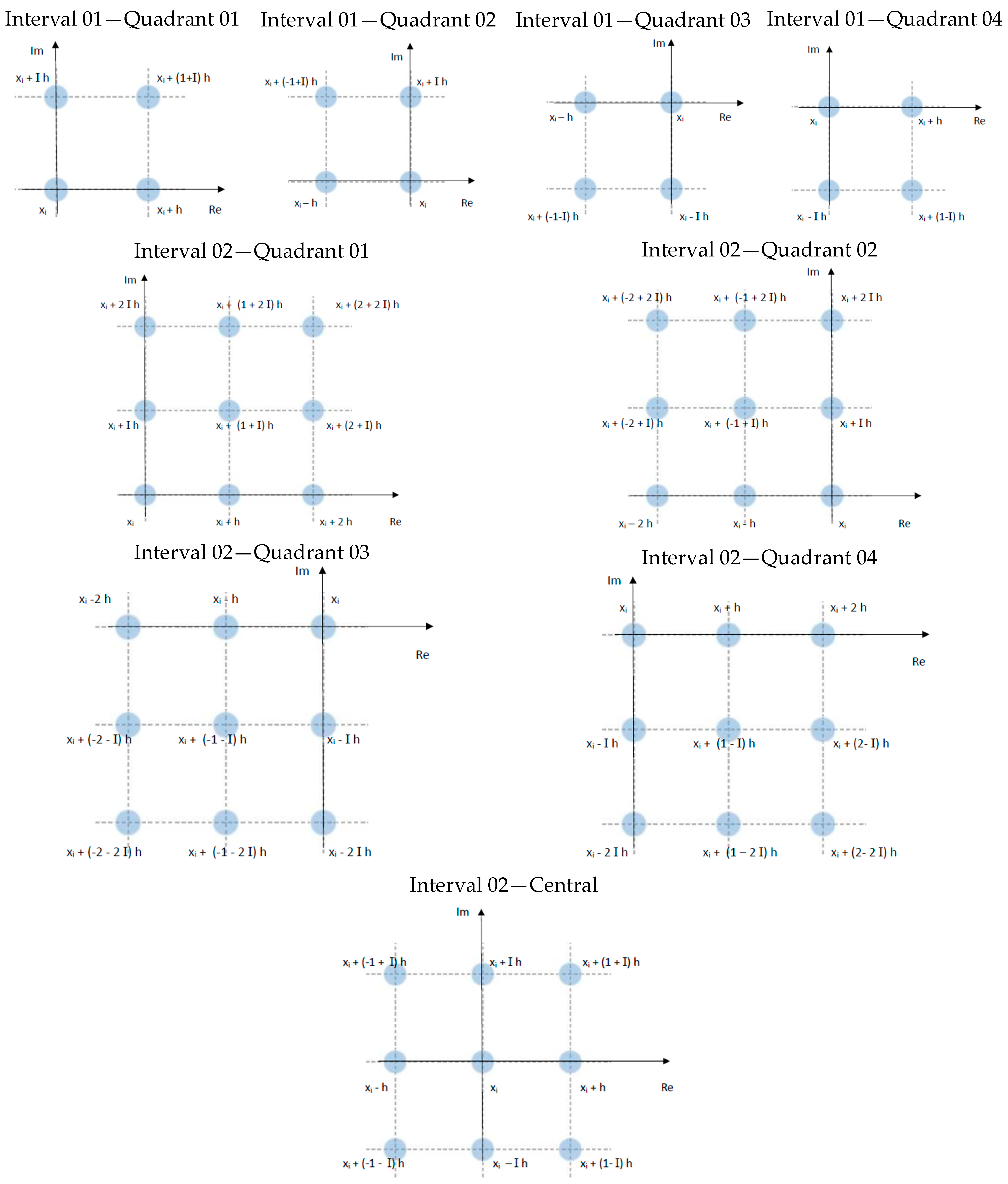
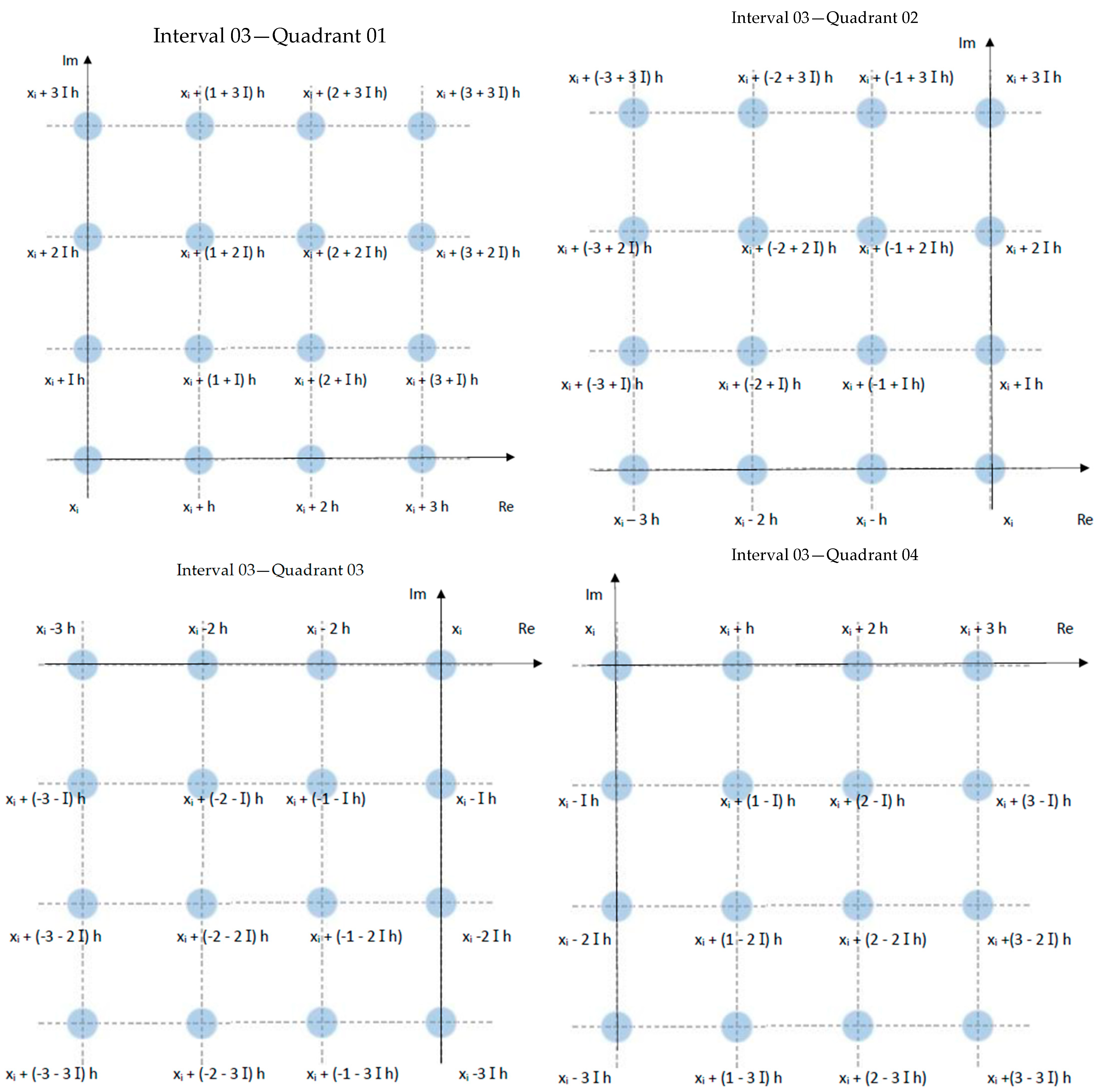
Define whether to use equations from the first, second, third, or fourth quadrants or central equations, thus having the discrete points of the finite difference formulas (depending on the need in the problem mesh).

(3)

Assemble the complex linear system using Taylor series (Equations (3)–(6)).

(4)

Solve the complex linear system and obtain approximations for the first derivative (Equations (11) and (12)).

(5)

Write the first derivative approximations obtained in terms of the Shift operator E, with complex powers (Section 6).

(6)

Define the derivative that must be calculated with the number of independent complex and real variables and the order of the derivative of each variable (depending on the differential equation to be solved).

(7)

Perform polynomial multiplication in terms of the Shift operator E to obtain the desired finite difference approximation (Section 4 and Section 6).

(8)

Perform an algebraic test of the formula obtained (Section 7).

(9)

Use the finite difference formula obtained in the practical example.

(10)

Apply the finite difference approximation with increasingly smaller increment steps until obtaining the desired precision and accuracy.

Table A12. Complex approximations used in solving the elasticity problem (part 1).

(a) $\frac{du\left(x_1\right)}{d{x}_1}=\frac{2u_{i1+I}+\left(1-I\right)u_{i1+1+I}+\left(-3+3I\right)u_{i1}-2I{u}_{i1+1}}{2∆x_1},O(∆x_1^3),Quadrant 1$ $\left(\mathrm{b}\right) \frac{du\left(x_1\right)}{d{x}_1}=\frac{-\left(1+I\right)u_{i1-1+I}-2u_{i1+I}-2I{u}_{i1-1}+\left(3+3I\right)u_{i1}}{2∆x_1},O(∆x_1^3),Quadrant 2$ $\left(\mathrm{c}\right) \frac{du\left(x_1\right)}{d{x}_1}=\frac{2I{u}_{i1-1}+\left(3-3I\right)u_{i1}+\left(-1+I\right)u_{i1-1-I}-2u_{i1-I}}{2∆x_1},O(∆x_1^3),Quadrant 3$ $\left(\mathrm{d}\right) \frac{du\left(x_1\right)}{d{x}_1}=\frac{-\left(3+3I\right)u_{i1}+2I{u}_{i1+1}+2u_{i1-I}+\left(1+I\right)u_{i1+1-I}}{2∆x_1},O(∆x_1^3),Quadrant 4$ (e) $\frac{du\left(x_1\right)}{d{x}_1}=\frac{-\left(1+I\right)u_{i1-1+I}-8I{u}_{i1+I}+\left(1-I\right)u_{i1+1+I}-8u_{i1-1}+8u_{i1+1}+\left(-1+I\right)u_{i1-1-I}+8I{u}_{i1-I}+\left(1+I\right)u_{i1+1-I}}{40∆x_1},O(∆x_1^8),Centered$

$\left(\mathrm{f}\right) \frac{d^{2}u\left(x_1\right)}{d{x}_1^2}=\frac{\left(-3+I\right)u_{i1+I}+2I{u}_{i1+1+I}-4I{u}_{i1}+\left(3+I\right)u_{i1+1}}{∆x_1^2},O(∆x_1^2),Quadrant 1$ $\left(\mathrm{g}\right) \frac{d^{2}u\left(x_1\right)}{d{x}_1^2}=\frac{-2I{u}_{i1-1+I}-\left(3+I\right)u_{i1+I}+\left(3-I\right)u_{i1-1}+4I{u}_{i1}}{∆x_1^2},O(∆x_1^2),Quadrant 2$ (h) $\frac{d^{2}u\left(x_1\right)}{d{x}_1^2}=\frac{\left(3+I\right)u_{i1-1}-4I{u}_{i1}+2I{u}_{i1-1-I}+\left(-3+I\right)u_{i1-I}}{∆x_1^2},O(∆x_1^2),Quadrant 3$ (i) $\frac{d^{2}u\left(x_1\right)}{d{x}_1^2}=\frac{4I{u}_{i1}+\left(3-I\right)u_{i1+1}-\left(3+I\right)u_{i1-I}-2I{u}_{i1+1-I}}{∆x_1^2},O(∆x_1^2),Quadrant 4$ (j) $\frac{d^{2}u\left(x_1\right)}{d{x}_1^2}=\frac{I{u}_{i1-1+I}-8u_{i1+I}-I{u}_{i1+1+I}+8u_{i1-1}+8u_{i1+1}-I{u}_{i1-1-I}-8u_{i1-I}+I{u}_{i1+1-I}}{20∆x_1^2},O(∆x_1^8),Centered$ $\begin{array}{c}\left(\mathrm{k}\right)\frac{d^{2}u\left(x_1\right)}{d{x}_1^2}=\frac{1}{800∆x_1^2}(u_{i1-2+2I}+(-8+8I)u_{i1-1+2I}-34u_{i1+2I}-(8+8I)u_{i1+1+2I}-I{u}_{i1+2+2I}+(8+8I)u_{i1-2+I}+\hfill \\ 64I{u}_{i1-1+I}-16u_{i1+I}-64I{u}_{i1+1+I}+(8-8I)u_{i1+2+I}+34u_{i1-2}+16u_{i1-1}+16u_{i1+1}+34u_{i1+2}+(8-8I)u_{i1-2-I}-\hfill \\ 64I{u}_{i1-1-I}-16u_{i1-I}+64I{u}_{i1+1-I}+(8+8I)u_{i1+2-I}-I{u}_{i1-2-2I}-(8+8I)u_{i1-1-2I}-34u_{i1-2I}+(-8+8I)u_{i1+1-2I}+\hfill \\ I{u}_{i1+2-2I}),O(∆x_1^8),Centered\hfill \end{array}$

and

Table A13. Complex approximations used in solving the elasticity problem (part 2).

$\begin{array}{c}\left(\mathrm{a}\right)\frac{{\partial }^{2}u\left(x_1,x_2\right)}{\partial x_1\partial x_2}=\frac{1}{800∆x_1∆x_2}(u_{i1-1+I,i2-1+I}+(-4+4I)u_{i1-1+I,i2+I}-u_{i1-1+I,i2+1+I}+(4+4I)u_{i1-1+I,i2-1}-(4+\hfill \\ 4I)u_{i1-1+I,i2+1}+u_{i1-1+I,i2-1-I}+(4-4I)u_{i1-1+I,i2-I}-I{u}_{i1-1+I,i2+1-I}+(-4+4I)u_{i1+I,i2-1+I}-32u_{i1+I,i2+I}-(4+\hfill \\ 4I)u_{i1+I,i2+1+I}+32I{u}_{i1+I,i2-1}-32I{u}_{i1+I,i2+1}+(4+4I)u_{i1+I,i2-1-I}+32u_{i1+I,i2-I}+(4-4I)u_{i1+I,i2+1-I}-u_{i1+1+I,i2-1+I}-\hfill \\ (4+4I)u_{i1+1+I,i2+I}-I{u}_{i1+1+I,i2+1+I}+(-4+4I)u_{i1+1+I,i2-1}+(4-4I)u_{i1+1+I,i2+1}+I{u}_{i1+1+I,i2-1-I}+(4+4I)u_{i1+1+I,i2-I}+\hfill \\ u_{i1+1+I,i2+1-I}+(4+4I)u_{i1-1,i2-1+I}+32I{u}_{i1-1,i2+I}+(-4+4I)u_{i1-1,i2+1+I}+32u_{i1-1,i2-1}-32u_{i1-1,i2+1}+(4-\hfill \\ 4I)u_{i1-1,i2-1-I}-32I{u}_{i1-1,i2-I}-(4+4I)u_{i1-1,i2+1-I}-(4+4I)u_{i1+1,i2-1+I}-32I{u}_{i1+1,i2+I}+(4-4I)u_{i1+1,i2+1+I}-\hfill \\ 32u_{i1+1,i2-1}+32u_{i1+1,i2+1}+(-4+4I)u_{i1+1,i2-1-I}+32I{u}_{i1+1,i2-I}+(4+4I)u_{i1+1,i2+1-I}+u_{i1-1-I,i2-1+I}+(4+\hfill \\ 4I)u_{i1-1-I,i2+I}+I{u}_{i1-1-I,i2+1+I}+(4-4I)u_{i1-1-I,i2-1}+(-4+4I)u_{i1-1-I,i2+1}-I{u}_{i1-1-I,i2-1-I}-(4+4I)u_{i1-1-I,i2-I}-\hfill \\ u_{i1-1-I,i2+1-I}+(4-4I)u_{i1-I,i2-1+I}+32u_{i1-I,i2+I}+(4+4I)u_{i1-I,i2+1+I}-32I{u}_{i1-I,i2-1}+32I{u}_{i1-I,i2+1}-(4+\hfill \\ 4I)u_{i1-I,i2-1-I}-32u_{i1-I,i2-I}+(-4+4I)u_{i1-I,i2+1-I}-I{u}_{i1+1-I,i2-1+I}+(4-4I)u_{i1+1-I,i2+I}+u_{i1+1-I,i2+1+I}-(4+\hfill \\ 4I)u_{i1+1-I,i2-1}+(4+4I)u_{i1+1-I,i2+1}-u_{i1+1-I,i2-1-I}+(-4+4I)u_{i1+1-I,i2-I}+I{u}_{i1+1-I,i2+1-I}),O(∆x_1^8∆x_2^8),Centered\hfill \end{array}$

$\left(\mathrm{b}\right) \frac{d^{3}u\left(x_1\right)}{d{x}_1^3}=\frac{\left(3-3I\right)u_{i1-1+I}+48I{u}_{i1+I}-\left(3+3I\right)u_{i1+1+I}-48u_{i1-1}+48u_{i1+1}+\left(3+3I\right)u_{i1-1-I}-48I{u}_{i1-I}+\left(-3+3I\right)u_{i1+1-I}}{40∆x_1^3},O(∆x_1^8),Centered$

$\left(\mathrm{c}\right) \frac{d^{4}u\left(x_1\right)}{d{x}_1^4}=\frac{3\left(-u_{i1-1+I}+16u_{i1+I}-u_{i1+1+I}+16u_{i1-1}-60u_{i1}+16u_{i1+1}-u_{i1-1-I}+16u_{i1-I}-u_{i1+1-I}\right)}{10∆x_1^4},O(∆x_1^8),Centered$ $\begin{array}{c}\left(\mathrm{d}\right)\frac{d^{4}u\left(x_1\right)}{d{x}_1^4}=\frac{1}{400∆x_1^4}(-u_{i1-2+2I}-16I{u}_{i1-1+2I}+66u_{i1+2I}+16I{u}_{i1+1+2I}-u_{i1+2+2I}+16I{u}_{i1-2+I}-128u_{i1-1+I}-\hfill \\ 128u_{i1+1+I}-16I{u}_{i1+2+I}+66u_{i1-2}+252u_{i1}+66u_{i1+2}-16I{u}_{i1-2-I}-128u_{i1-1-I}-128u_{i1+1-I}+16I{u}_{i1+2-I}-u_{i1-2-2I}+\hfill \\ 16I{u}_{i1-1-2I}+66u_{i1-2I}-16I{u}_{i1+1-2I}-u_{i1+2-2I}),O(∆x_1^8),Centered\hfill \end{array}$

$\begin{array}{c}\left(\mathrm{e}\right)\frac{{\partial }^{4}u\left(x_1,x_2\right)}{\partial x_1^2\partial x_2^2}=\frac{1}{400∆x_1^2∆x_2^2}(-u_{i1-1+I,i2-1+I}-8I{u}_{i1-1+I,i2+I}+u_{i1-1+I,i2+1+I}+8I{u}_{i1-1+I,i2-1}+8I{u}_{i1-1+I,i2+1}+u_{i1-1+I,i2-1-I}-\hfill \\ 8I{u}_{i1-1+I,i2-I}-u_{i1-1+I,i2+1-I}-8I{u}_{i1+I,i2-1+I}+64u_{i1+I,i2+I}+8I{u}_{i1+I,i2+1+I}-64u_{i1+I,i2-1}-64u_{i1+I,i2+1}+8I{u}_{i1+I,i2-1-I}+\hfill \\ 64u_{i1+I,i2-I}-8I{u}_{i1+I,i2+1-I}+u_{i1+1+I,i2-1+I}+8I{u}_{i1+1+I,i2+I}-u_{i1+1+I,i2+1+I}-8I{u}_{i1+1+I,i2-1}-8I{u}_{i1+1+I,i2+1}-\hfill \\ u_{i1+1+I,i2-1-I}+8I{u}_{i1+1+I,i2-I}+u_{i1+1+I,i2+1-I}+8I{u}_{i1-1,i2-1+I}-64u_{i1-1,i2+I}-8I{u}_{i1-1,i2+1+I}+64u_{i1-1,i2-1}+64u_{i1-1,i2+1}-\hfill \\ 8I{u}_{i1-1,i2-1-I}-64u_{i1-1,i2-I}+8I{u}_{i1-1,i2+1-I}+8I{u}_{i1+1,i2-1+I}-64u_{i1+1,i2+I}-8I{u}_{i1+1,i2+1+I}+64u_{i1+1,i2-1}+64u_{i1+1,i2+1}-\hfill \\ 8I{u}_{i1+1,i2-1-I}-64u_{i1+1,i2-I}+8I{u}_{i1+1,i2+1-I}+u_{i1-1-I,i2-1+I}+8I{u}_{i1-1-I,i2+I}-u_{i1-1-I,i2+1+I}-8I{u}_{i1-1-I,i2-1}-\hfill \\ 8I{u}_{i1-1-I,i2+1}-u_{i1-1-I,i2-1-I}+8I{u}_{i1-1-I,i2-I}+u_{i1-1-I,i2+1-I}-8I{u}_{i1-I,i2-1+I}+64u_{i1-I,i2+I}+8I{u}_{i1-I,i2+1+I}-64u_{i1-I,i2-1}-\hfill \\ 64u_{i1-I,i2+1}+8I{u}_{i1-I,i2-1-I}+64u_{i1-I,i2-I}-8I{u}_{i1-I,i2+1-I}-u_{i1+1-I,i2-1+I}-8I{u}_{i1+1-I,i2+I}+u_{i1+1-I,i2+1+I}+8I{u}_{i1+1-I,i2-1}+\hfill \\ 8I{u}_{i1+1-I,i2+1}+u_{i1+1-I,i2-1-I}-8I{u}_{i1+1-I,i2-I}-u_{i1+1-I,i2+1-I}),O(∆x_1^8∆x_2^8),Centered\hfill \end{array}$

in Appendix A show the complex finite difference formulas utilized in solving the problem.

The implicit method was used to solve the problem by finite differences, making Δr = 0.001 m and Δθ = 0.01 rad, and then comparing with Δr = 0.0001 m and Δθ = 0.001 rad using 8 decimal places. Although the edges were circular, as the steps were very small and, consequently, the elements as well, the Control–Volume Approach or Volume–Integral Approach (a technique used for an irregularly shaped boundary, where weighting coefficients are applied to account for the nonuniform spacing in the vicinity of the nonrectangular boundary) were not used [1,2,3].

The computational solution of the problem was performed, and the linear system was solved by an iterative method. Figure 5 graphically shows the results, which were compared with the analytical solutions and were successful up to the eighth decimal place of precision (ξ ≤ 10⁻⁸). To gain computational efficiency, only the nodes where x² + y² were between the internal radius R1² (0.02²) and the external radius R2² (0.04²) were activated for the calculation. Each node is a real value of the incognita (ϕ) Airy’s stress function or a complex value of the incognita (Z) Westergaard’s stress function, but it is also a finite difference equation. At the edge of the boundary of the inner radius and outer radius, an increase in the grid of eight radial lines was provided for the stress boundary conditions. Thus, the number of unknowns (nodes) was equal to the number of equations in a large linear system that can be solved by Gauss–Seidel-type iterative techniques [2,31]. For this example of compression rings, the exact value of the analytical solution of the differential equation at each position, x and y, was also calculated. Thus, the error of using the finite difference method was obtained in the real case and in the complex case.

The results obtained by finite differences were compared with the analytical solution up to an error of less than eight decimal places. This example demonstrated the effectiveness of the finite difference method in accurately solving an engineering application involving fourth-order differential equations and circular geometry [26].

Both in the real model with the Airy function and in the complex model with the Westergaard function, the finite difference method was successful in obtaining the stress diagrams. No significant visual differences were observed between the real solution and the complex solution.

Table 3. Comparison of the real solution with the complex solution of the Theory of Elasticity problem of circular rings in compression.

Step or Increment of Cartesian Coordinates x and y—Δx or Δy (m)	Step or Increment of Polar Coordinates Radial Distance—Δr (m)	Step or Increment of Polar Coordinates Polar Angle—Δθ (rad)	Average Stresses Error between the Exact Value and the Real Solution Due to Finite Differences at the Mesh Nodes—σ or τ (Pa)	Average Stresses Error between the Exact Value and the Complex Solution Due to Finite Differences at the Mesh Nodes—σ or τ (Pa)
h = 0.1	0.14142	0.07854	0.02805	0.006871
h = 0.01	0.014142	0.007854	2.4463 × 10−6	5.8212 × 10−11
h = 0.001	0.0014142	0.0007854	7.7650 × 10−10	8.5163 × 10−19
h = 10−4	1.14142 × 10−4	7.854 × 10−5	1.5339 × 10−14	1.2798 × 10−27
h = 10−5	1.14142 × 10−5	7.854 × 10−6	7.4519 × 10−18	6.7628 × 10−35
h = 10−6	1.14142 × 10−6	7.854 × 10−7	1.7867 × 10−22	8.6599 × 10−43

shows a comparison of the errors of the real solution in relation to the errors of the complex solution [23]. It should be noted that the complex solution obtained fewer errors, being considered much better than the real solution.

To date, we do not have a full understanding of why the complex solution is more accurate than the real solution. However, it is believed that the order of error in complex finite difference formulas is greater than that used in real finite difference formulas. Another reason comes from the modulus of the coefficients of the terms in complex finite difference equations being smaller than the real coefficients, reducing rounding errors in mathematical operations.

Finite difference formulas in the complex plane are in general more accurate than finite difference formulas in the real domain [17,18,19,20]. The reasons for this are that complex derivatives depend equally on data from all directions around the point, i.e., stencils must not extend very far, only along a line, and the Cauchy–Riemann equations impose restrictions on the range of functions that need to be considered. Even as stencil sizes and orders of accuracy increase, complex planar finite difference stencils continue to extract their key information from a very small neighborhood of the point of interest. By using standard finite difference approximations along the real axis and increasing the stencil width and precision order to a fixed derivative, the weights converge to a limit, known as the pseudospectral method. This contrasts with traditional pseudospectral methods which, with their slow algebraic decay of weights, rely on distant data, even when approximating local operators as derivatives. It seems that the derivative at a point cannot depend on the direction of approach in the complex plane, resulting in greater stability for the finite difference method. Holding a stencil size fixed and increasing the order p of the derivative $d^p/{dz}^p$ (as far as the stencil size permits) will typically make the weights (following the leading factor $1/h^p$) increase rapidly. The Cauchy–Riemann equations also seemed to smooth the variations of finite differences in the complex domain, which improved the numerical precision and accuracy of numerical solutions of differential equations. The Euler–Maclaurin approximations benefited from a compensatory decrease in the magnitude of the coefficients for successive terms. If a very high-order derivative is to be approximated, algorithms based on Cauchy integrals may be preferable to finite difference approximations. Another option could be to find sets of finite difference weights where some orders of precision have been traded off against reductions in the magnitude of the weights. This has been used successfully in contexts such as numerical quadrature and in cases of Gregory-type and Newton–Cotes-type formulas, respectively.

Another issue that helps in the use of complex finite difference approximations is the square increase in the points used per interval. Thus, a spacing interval uses two points in the real case and four points in the complex case, two intervals uses three points in the real case and nine points in the complex case, three intervals uses four points in the real case and sixteen points in the complex case, and so on. This increases the precision and error order of the finite difference approximation and decreases the absolute value of the coefficient values of the finite difference approximations.

Table 4. Comparison of the precision of numerical resolution of differential equations between the different grids in the complex plane.

Grid or Set of Points of the Main Stencil Used in the Numerical Resolution of the Stress Calculation Problem:	Average Stresses Error between the Exact Value and the Complex Solution Due to Finite Differences at the Mesh Nodes with Step of Cartesian Coordinates x and y Equal to:
	h = 0.1	h = 0.01	h = 0.001	h = 10−4	h = 10−5
Square with Interval 01—Quadrant 01—Table A4a	2.04 × 102	6.83 × 10−1	9.59 × 10−4	4.50 × 10−7	9.74 × 10−10
Square with Interval 01—Quadrant 02—Table A5a	3.88 × 102	8.91 × 10−1	7.38 × 10−4	1.75 × 10−8	2.48 × 10−10
Square with Interval 01—Quadrant 03—Table A6a	3.88 × 102	3.36 × 10−1	6.95 × 10−4	4.28 × 10−7	1.29 × 10−10
Square with Interval 01—Quadrant 04—Table A7a	2.27 × 10	1.26 × 10−1	1.40 × 10−4	4.74 × 10−7	1.38 × 10−10
Square with Interval 02—Quadrant 01—Table A4b	3.81 × 10−3	3.37 × 10−11	4.86 × 10−20	5.67 × 10−27	7.91 × 10−35
Square with Interval 02—Quadrant 02—Table A5b	3.17 × 10−3	7.21 × 10−11	6.76 × 10−19	7.29 × 10−27	4.08 × 10−35
Square with Interval 02—Quadrant 03—Table A6b	8.40 × 10−3	3.19 × 10−11	6.46 × 10−19	5.17 × 10−27	2.78 × 10−35
Square with Interval 02—Quadrant 04—Table A7b	7.78 × 10−3	6.94 × 10−11	4.22 × 10−19	2.95 × 10−27	7.70 × 10−35
Square with Interval 02—Central—Table A8a	3.74 × 10−3	4.45 × 10−11	3.00 × 10−19	3.47 × 10−27	1.45 × 10−35
Square with Interval 03—Quadrant 01—Table A4c	5.93× 10−10	4.49 × 10−25	7.82 × 10−40	4.18 × 10−55	3.33 × 10−71
Square with Interval 03—Quadrant 02—Table A5c	9.28 × 10−10	4.63 × 10−25	2.67 × 10−40	6.06 × 10−55	8.83 × 10−70
Square with Interval 03—Quadrant 03—Table A6c	8.08× 10−10	4.49 × 10−25	1.47 × 10−40	6.56 × 10−57	3.80 × 10−70
Square with Interval 03—Quadrant 04—Table A7c	9.42 × 10−10	5.81 × 10−25	2.63 × 10−40	7.71 × 10−55	2.56 × 10−70
Square with Interval 04—Quadrant 01—Table A4d	2.85 × 10−19	4.90 × 10−43	3.28 × 10−67	3.87 × 10−93	9.37 × 10−115
Square with Interval 04—Quadrant 02—Table A5d	2.55 × 10−19	2.25 × 10−43	6.99 × 10−69	4.82 × 10−91	7.77 × 10−115
Square with Interval 04—Quadrant 03—Table A6d	5.51 × 10−19	5.93 × 10−43	2.88 × 10−67	6.04 × 10−91	3.07 × 10−115
Square with Interval 04—Quadrant 04—Table A7d	4.76 × 10−19	2.18 × 10−43	5.04 × 10−67	9.71 × 10−92	3.72 × 10−115
Square with Interval 04—Central—Table A8b	4.61 × 10−19	1.73 × 10−43	2.84 × 10−67	6.20 × 10−92	1.63 × 10−116
Square with Interval 06—Central—Table A8c	3.24 × 10−43	8.05 × 10−92	2.40 × 10−140	2.89 × 10−187	4.55 × 10−235
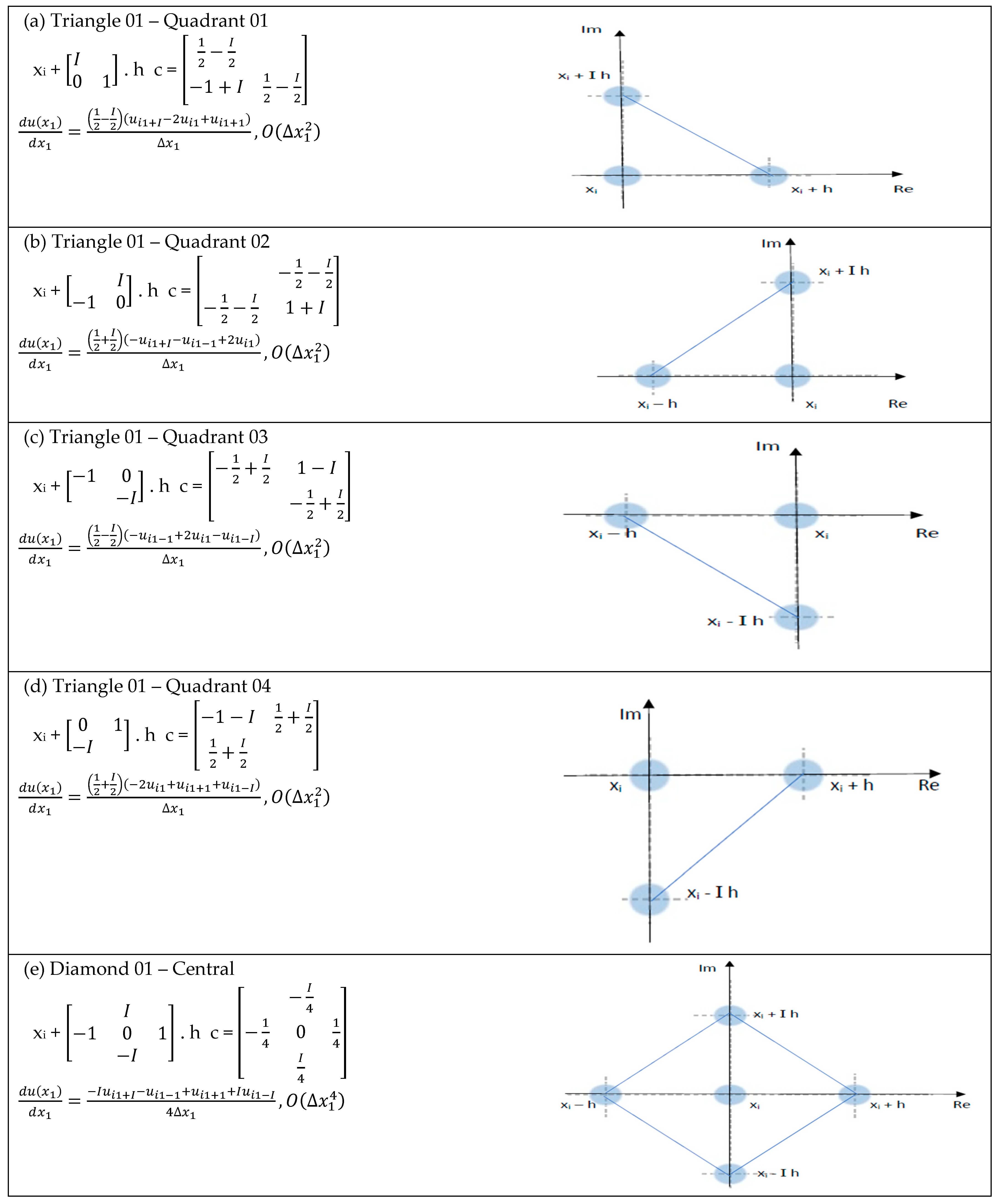
Triangle 01—Quadrant 01—Figure A1a	2.72 × 103	2.49 × 10	5.95 × 10−1	4.75 × 10−4	2.20 × 10−5
Triangle 01—Quadrant 02—Figure A1b	5.88 × 103	9.82 × 10	1.92 × 10−1	7.83 × 10−3	6.13 × 10−5
Triangle 01—Quadrant 03—Figure A1c	5.08 × 103	1.60 × 10	9.20 × 10−1	5.90 × 10−3	6.71 × 10−5
Triangle 01—Quadrant 04—Figure A1d	8.42 × 103	5.53 × 10	1.41 × 10−1	6.50 × 10−3	2.90 × 10−5
Diamond 01—Central—Figure A1e	2.56 × 100	8.22 × 10−4	4.12 × 10−7	2.37 × 10−11	2.71 × 10−15
Triangle 02—Quadrant 01—Figure A2a	9.28 × 100	2.52 × 10−5	9.63 × 10−10	3.15 × 10−15	8.28 × 10−20
Triangle 02—Quadrant 02—Figure A2b	8.34 × 100	1.43 × 10−5	1.60 × 10−10	6.00 × 10−15	8.71 × 10−20
Triangle 02—Quadrant 03—Figure A2c	5.20 × 100	3.53 × 1005	2.10 × 10−10	4.60 × 10−15	2.78 × 10−21
Triangle 02—Quadrant 04—Figure A3a	1.81 × 100	6.62 × 10−5	7.90 × 10−10	3.78 × 10−15	1.78 × 10−20
Diamond 02—Central—Figure A3b	2.09 × 10−6	2.57 × 10−17	3.88 × 10−28	1.10 × 10−39	2.79 × 10−50
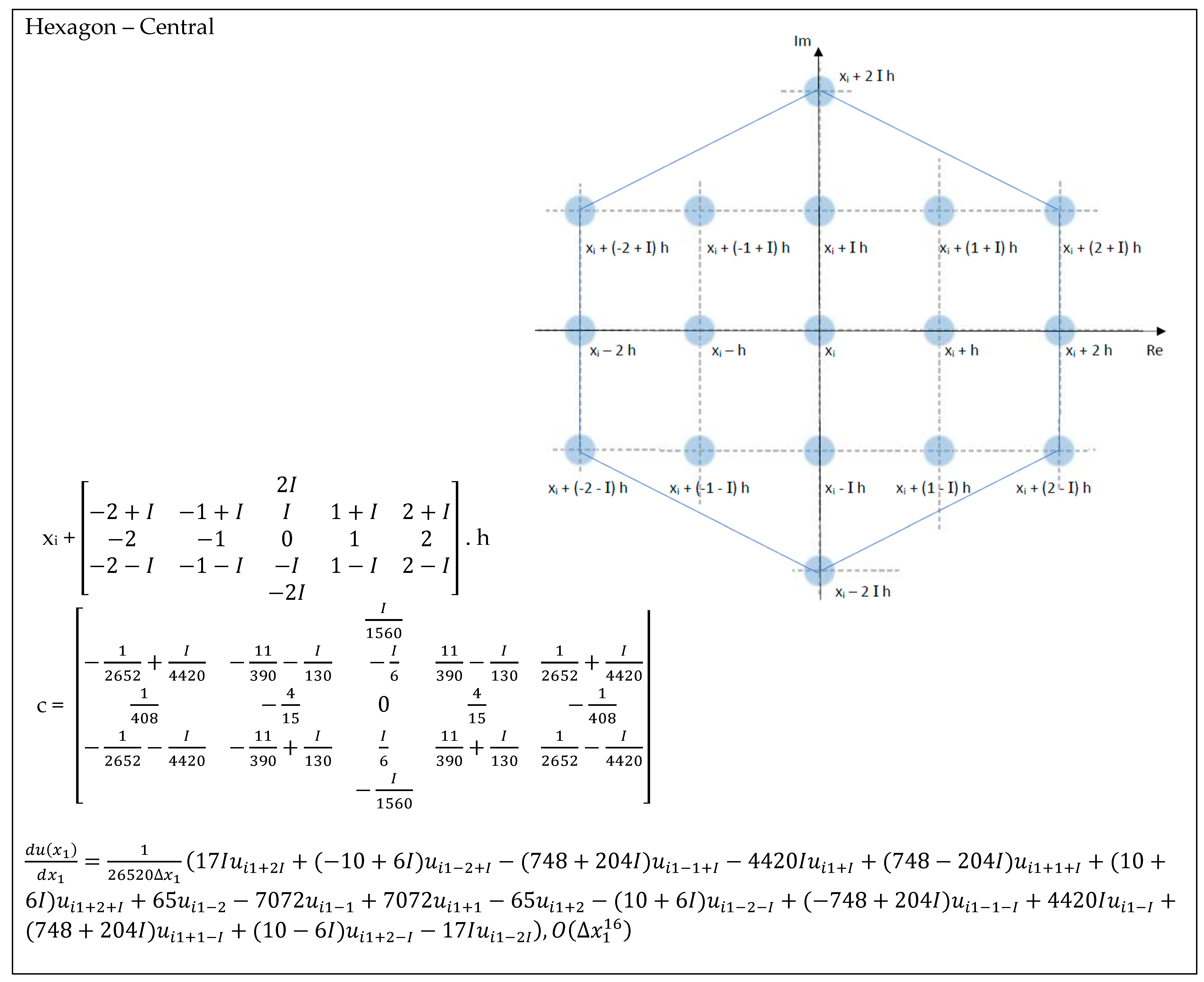
Hexagon—Central—Figure A4	2.96 × 10−12	2.63 × 10−27	1.18 × 10−43	1.59 × 10−59	2.87 × 10−75
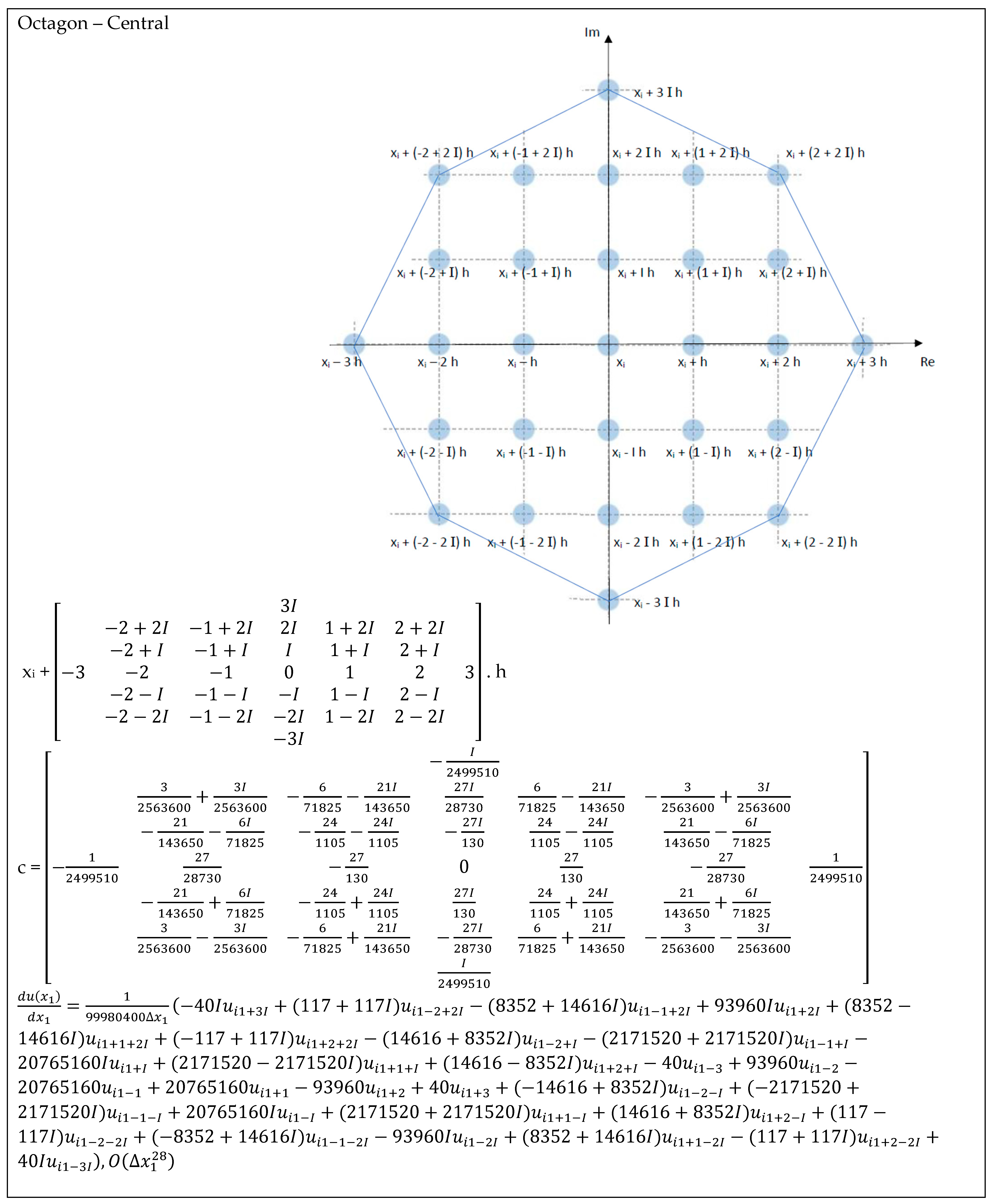
Octagon—Central—Figure A5	2.00 × 10−23	1.50 × 10−51	1.59 × 10−79	2.88 × 10−107	3.03 × 10−135
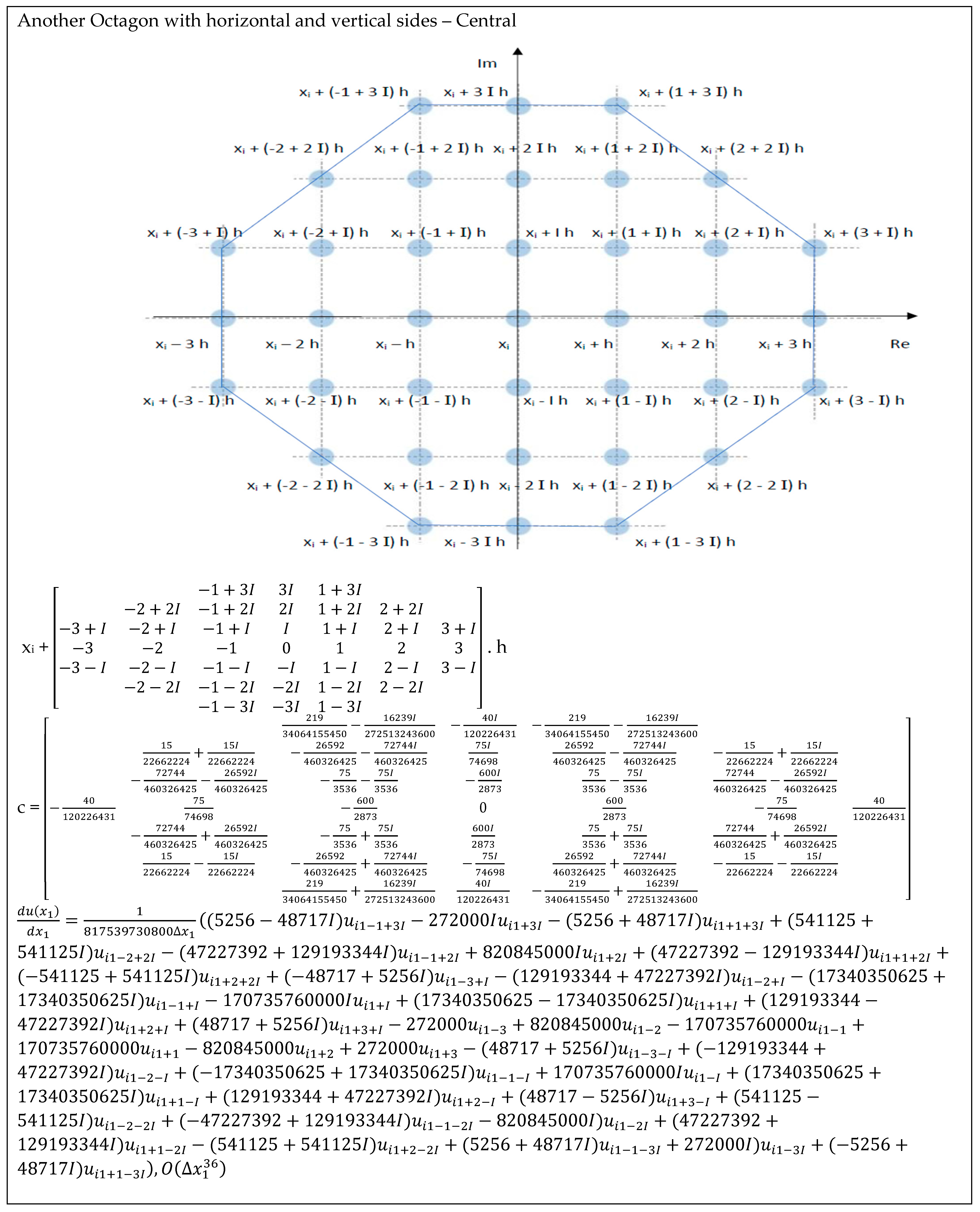
Another Octagon with horizontal and vertical sides—Central—Figure A6	1.22 × 10−32	7.50 × 10−68	1.90 × 10−103	2.38 × 10−139	8.11 × 10−176
Dodecagon with horizontal and vertical sides—Central—Figure A7 and Figure A8	1.32 × 10−55	1.51 × 10−115	1.10 × 10−175	7.71 × 10−236	1.73 × 10−296

shows a comparison between the various finite difference formulas used in numerically solving the stress problem. Note that only the main finite difference approximations for the fourth-order derivatives have been changed, as the initial and boundary conditions that use Dirichlet, Neumann, or second- and third-order derivatives are the same finite difference equations.

Comparing finite difference approximations in the complex field, it was noted that the central equations and more points had advantages, as well as equations that have geometric symmetry between the four quadrants of the complex plane and that try to get closer to circles centered at the origin. In other words, the symmetrical and regular distribution of the stencils helps to obtain more precise and accurate finite difference approximations.

Many other applications and tests of finite difference derivative approximations are provided in the literature [21,32,33,34,35,36,37,38,39,40,41].

10. Conclusions

The finite difference method is an important numerical method for solving both differential equations and computer simulations. For the same order of error, approximations of derivatives by finite differences were obtained with a smaller absolute value of the coefficients in the complex domain than in the real domain, which reduced the propagation of the rounding error. Finite difference formulas in the complex plane are in general more precise and accurate than finite difference formulas in the real domain. Furthermore, a much greater diversity of finite difference equations was obtained in the complex field than in the real domain, in all orders of errors and for the most varied boundary and initial conditions. The work is innovative, with a complex potentiation of numerical operators.

It was possible in the complex domain to obtain finite difference approximations of a high order of error or precision with few points of the function, even reaching equations with an error order of O(hⁿ) and with only n points of the function. The reduced number of points in the finite difference approximation was important, especially in the boundary and initial conditions. Obtaining approximations of derivatives with a high order of error improved the precision of the numerical resolution of differential equations and reduced the computational effort in the finite difference method. The research was successful in obtaining approximations of derivatives by finite differences in the complex domain with a high order of error and with few points in the equations, which increased the applicability of the finite difference method and reduced restrictions on its use.

Due to the complex boundary and initial conditions that appear in structural engineering and solid mechanics problems, a large number of finite difference derivative approximations are necessary to solve the problems with accuracy. This work showed that, with modern microcomputers and a database with several finite difference equations for derivative approximations, many structural analysis problems can be solved with high numerical precision by applying the finite difference method.

This paper showed that although it is outdated, the finite difference method is still very important and cannot be abandoned. It is believed that it is best to use the finite difference method in conjunction with other numerical methods of solving differential equations, such as the finite element method and the boundary element method. The finite differences method presents high stability and easy application in many practical cases of problems involving differential equations, mainly problems involving long time series or sequences and derived from high orders or problems with part of the geometry having a simpler rectangular shape and large areas and volumes with homogeneous media. In these cases, the finite difference method has great advantages.

This article showed how structural mechanics problems can be solved using the finite difference method in the complex domain. Furthermore, it showed how advantageous it is to use complex mathematical models in relation to models in the real domain. Westergaard stress functions are more general and comprehensive than Airy’s stress function, and the finite difference method, which is a numerical method widely used in computer simulations, seemed to work better in the complex plane.

This paper showed how to obtain, in a simple and practical way, finite difference equations that perform approximations of the calculation of derivatives with high orders of error. Correctly using these finite difference equations, we obtained precise and exact solutions of differential equations in practical science and engineering problems. Thus, the finite difference method remains a powerful and robust numerical method for solving differential equation problems that efficiently utilizes recent computational advances in hardware and software.

Since finite differences formulas in the complex plane are generally considerably more accurate than traditional ones that use function values only along the real axis, it is concluded that it may be advantageous to solve differential equation problems using the finite difference method with variables in the complex domain instead of the real domain, which can even generalize many mathematical models of physical and engineering phenomena. The application of the finite difference method in the complex plane can be used to determine whether a variable is better modeled as belonging to the real domain or the complex domain in the study or analysis of a certain phenomenon.

As Supplementary Material of the paper, many of the approximations of derivatives by complex finite differences are presented in a PDF (https://zenodo.org/records/10901007, accessed on 3 April 2024).

References

- Hoffman, J.D.; Hoffman, J.D.; Frankel, S. Numerical Methods for Engineers and Scientists; CRC Press: Boca Raton, FL, USA, 2018. [Google Scholar] [CrossRef]
- Steven, C.C. Applied Numercial Methods with MATLAB for Engineers and Scientist; McGraw Hill: New York, NY, USA, 2013; Volume 53. [Google Scholar]
- Chapra, S.C.; Canale, R.P. Numerical Methods for Engineers, 2nd ed.; New Age International: New Delhi, India, 2006. [Google Scholar]
- Nayak, G.C. Applied Numerical Methods, B. Carnahan, H.A. Lither and J. O. Wilkes, Wiley, New York, 1969. No. of Pages: 604. Price: £6·60. Int. J. Numer. Methods Eng. 1972, 4, 599–600. [Google Scholar] [CrossRef]
- Seiler, M.C.; Seiler, F.A. Numerical Recipes in C: The Art of Scientific Computing. Risk Anal. 1989, 9, 415–416. [Google Scholar] [CrossRef]
- Dukkipati, R.V. Numerical Methods; Courier Corporation: New Delhi, India, 2010. [Google Scholar]
- Chapra, S.C. Métodos Numéricos Para Ingenieros; McGraw Hill: New York, NY, USA, 2011. [Google Scholar]
- Chen, Q.; Wang, P.; Zhu, D. A Second-Order Finite-Difference Method for Derivative-Free Optimization. J. Math. 2024, 2024, 1947996. [Google Scholar] [CrossRef]
- Chelnokov, Y.N. Quaternion Methods and Models of Regular Celestial Mechanics and Astrodynamics. Appl. Math. Mech. 2022, 43, 21–80. [Google Scholar] [CrossRef]
- Roberts, J.L. A Method for Calculating Meshless Finite Difference Weights. Int. J. Numer. Methods Eng. 2008, 74. [Google Scholar] [CrossRef]
- Khan, I.R.; Ohba, R. Closed-Form Expressions for the Finite Difference Approximations of First and Higher Derivatives Based on Taylor Series. J. Comput. Appl. Math. 1999, 107, 179–193, Corrigendum in J. Comput. Appl. Math. 2001, 130, 385. [Google Scholar] [CrossRef]
- Khan, I.R.; Ohba, R.; Hozumi, N. Mathematical Proof of Closed Form Expressions for Finite Difference Approximations Based on Taylor Series. J. Comput. Appl. Math. 2003, 150, 303–309. [Google Scholar] [CrossRef]
- Khan, I.R.; Ohba, R. Taylor Series Based Finite Difference Approximations of Higher-Degree Derivatives. J. Comput. Appl. Math. 2003, 154, 115–124. [Google Scholar] [CrossRef]
- Khan, I.R.; Ohba, R. New Finite Difference Formulas for Numerical Differentiation. J. Comput. Appl. Math. 2000, 126, 269–276. [Google Scholar] [CrossRef]
- Li, J. General Explicit Difference Formulas for Numerical Differentiation. J. Comput. Appl. Math. 2005, 183, 29–52. [Google Scholar] [CrossRef]
- Feagin, T. High-Order Explicit Runge-Kutta Methods Using m-Symmetry. Neural Parallel Sci. Comput. 2012, 20, 437–458. [Google Scholar]
- Fornberg, B. Infinite-Order Accuracy Limit of Finite Difference Formulas in the Complex Plane. IMA J. Numer. Anal. 2023, 43, 3055–3072. [Google Scholar] [CrossRef]
- Fornberg, B.; Piret, C. Computation of Fractional Derivatives of Analytic Functions. J. Sci. Comput. 2023, 96, 79. [Google Scholar] [CrossRef]
- Fornberg, B. Finite Difference Formulas in the Complex Plane. Numer. Algorithms 2022, 90, 1305–1326. [Google Scholar] [CrossRef]
- Abrahamsen, D.; Fornberg, B. Solving the Korteweg-de Vries Equation with Hermite-Based Finite Differences. Appl. Math. Comput. 2021, 401, 126101. [Google Scholar] [CrossRef]
- Li, T.; Wang, Q.W. Structure Preserving Quaternion Full Orthogonalization Method with Applications. Numer. Linear Algebra Appl. 2023, 30, e2495. [Google Scholar] [CrossRef]
- SEM. Handbook on Experimental Mechanics. Exp. Tech. 1989, 13, 21. [Google Scholar] [CrossRef]
- Tokovyy, Y.V.; Hung, K.M.; Ma, C.C. Determination of Stresses and Displacements in a Thin Annular Disk Subjected to Diametral Compression. J. Math. Sci. 2010, 165, 342–354. [Google Scholar] [CrossRef]
- Markides, C.F.; Kourkoulis, S.K. Stresses and Displacements in an Elliptically Perforated Circular Disc under Radial Pressure. Eng. Trans. 2014, 62, 131–169. [Google Scholar]
- Vasil’ev, V.V.; Fedorov, L.V. Stress functions in elasticity theory. Mech. Solids 2022, 57, 770–778. [Google Scholar] [CrossRef]
- Sadd, M.H. Elasticity: Theory, Applications, and Numerics; Elsevier: Amsterdam, The Netherlands, 2020. [Google Scholar] [CrossRef]
- Jiang, Y.; Pu, C. The Problem of I–II Combined Plane Crack Solved with Westergaard Stress Function. Mech. Eng. 2020, 42, 504–507. [Google Scholar] [CrossRef]
- Dumont, N.A.; Mamani, E.Y. Generalized Westergaard Stress Functions as Fundamental Solutions. CMES Comput. Model. Eng. Sci. 2011, 78, 109–149. [Google Scholar]
- Sun, C.T.; Farris, T.N. On the Completeness of the Westergaard Stress Functions. Int. J. Fract. 1989, 40, 73–77. [Google Scholar] [CrossRef]
- Leven, M.M. Discussion: “A New Method to ‘Lock-In’ Elastic Effects for Experimental Stress Analysis” (Dally, J.W., Durelli, A.J., and Riley, W.F., 1958, ASME J. Appl. Mech., 25, Pp. 189–195). J. Appl. Mech. 1959, 26, 152. [Google Scholar] [CrossRef]
- Clough, D.E.; Chapra, S.C. Introduction to Engineering and Scientific Computing with Python; Informa UK Limited: London, UK, 2022. [Google Scholar] [CrossRef]
- Magalhães, P.A.A. New Equations for Phase Evaluation in Measurements with an Arbitrary but Constant Phase Shift between Captured Intensity Signs. Opt. Eng. 2009, 48, 113602. [Google Scholar] [CrossRef]
- Cunha, P.P.S.R.; da Souza, P.M.; Valente, L.C.; Mello, G.M.V.; de Junior, P.A.A.M. Analysis of Induced Drag and Vortex at the Wing Tip of a Blended Wing Body Aircraft. Int. J. Adv. Eng. Res. Sci. 2018, 5, 7–9. [Google Scholar] [CrossRef]
- Magalhaes, P.A.A.; Magalhaes, C.A. Higher-Order Newton-Cotes Formulas. J. Math. Stat. 2010, 6, 193–204. [Google Scholar] [CrossRef]
- Almeida Magalhaes, C.; Americo Almeida Magalhaes, P. New Numerical Methods for the Photoelastic Technique with High Accuracy. J. Appl. Phys. 2012, 112, 083111. [Google Scholar] [CrossRef]
- Lamon, G.P.S.; Magalhães Júnior, P.A.A.; Carneiro, J.R.G. Cole type Pitot tube, discharge factor survey and calibration. Meas. Sens. 2024, 33, 101152. [Google Scholar] [CrossRef]
- López-Pérez, A.; Febrero-Bande, M.; González-Manteiga, W. Parametric estimation of diffusion processes: A review and comparative study. Mathematics 2021, 9, 859. [Google Scholar] [CrossRef]
- Berdyshev, A.; Baigereyev, D.; Boranbek, K. Numerical Method for Fractional-Order Generalization of the Stochastic Stokes–Darcy Model. Mathematics 2023, 11, 3763. [Google Scholar] [CrossRef]
- Pekmen Geridonmez, B.P.; Oztop, H.F. Entropy Generation Due to Magneto-Convection of a Hybrid Nanofluid in the Presence of a Wavy Conducting Wall. Mathematics 2022, 10, 4663. [Google Scholar] [CrossRef]
- Sun, J.; Wang, L.; Gong, D. A Joint Optimization Algorithm Based on the Optimal Shape Parameter–Gaussian Radial Basis Function Surrogate Model and Its Application. Mathematics 2023, 11, 3169. [Google Scholar] [CrossRef]
- Alahmadi, R.A.; Raza, J.; Mushtaq, T.; Abdelmohsen, S.A.M.; RGorji, M.; Hassan, A.M. Optimization of MHD Flow of Radiative Micropolar Nanofluid in a Channel by RSM: Sensitivity Analysis. Mathematics 2023, 11, 939. [Google Scholar] [CrossRef]