
Development of Mathematical Models for Industrial Processes Using Dynamic Neural Networks


Abstract
:1. Introduction
2. Materials and Methods
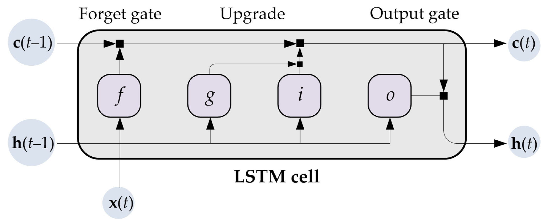
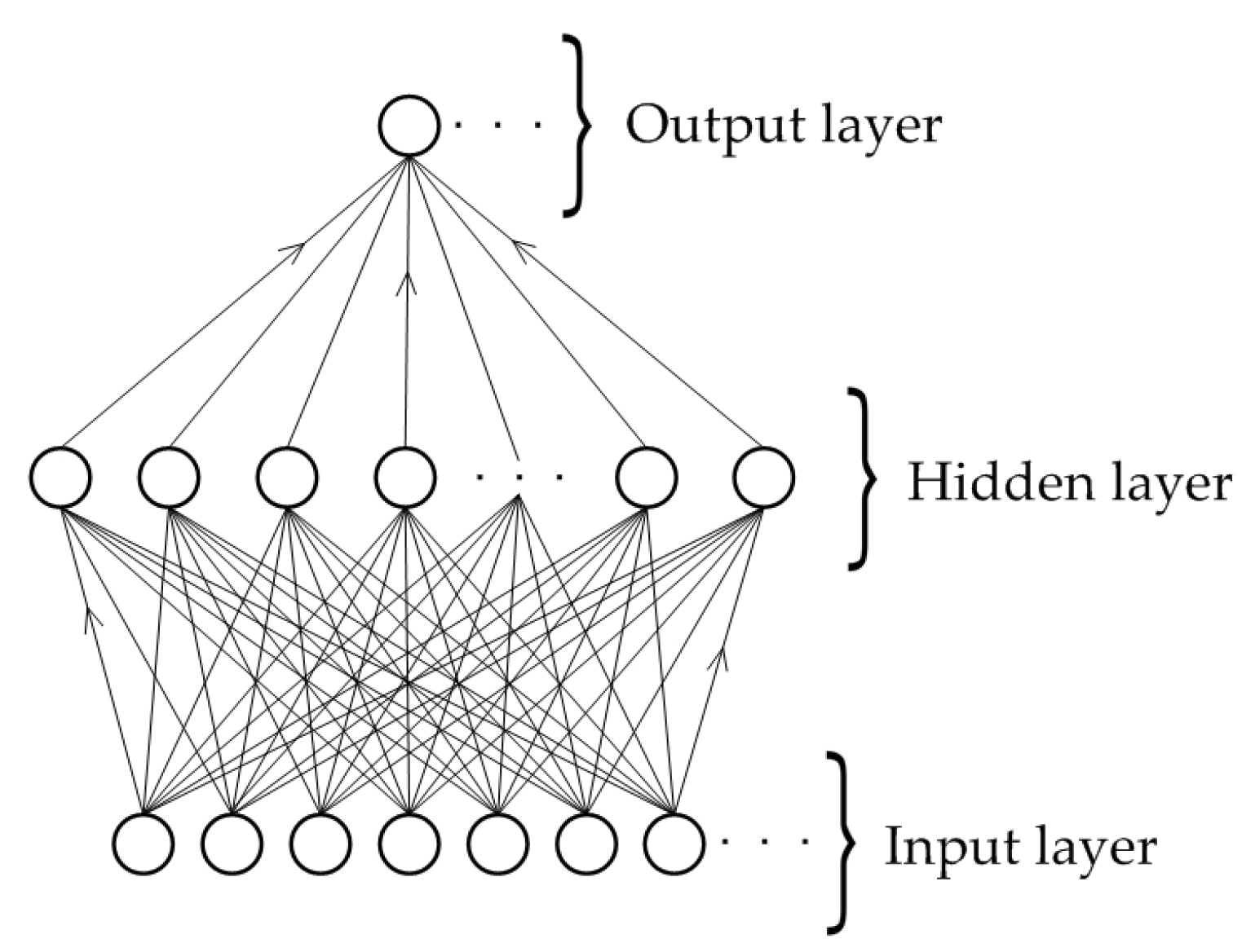
2.1. Theoretical Background
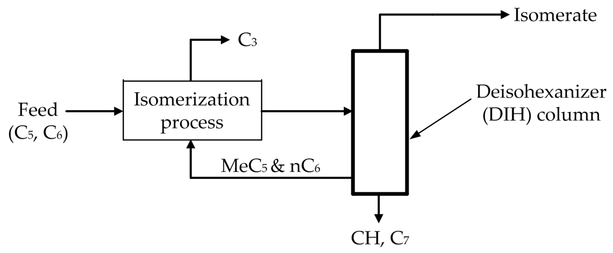
2.2. Process Description
2.3. Model Development
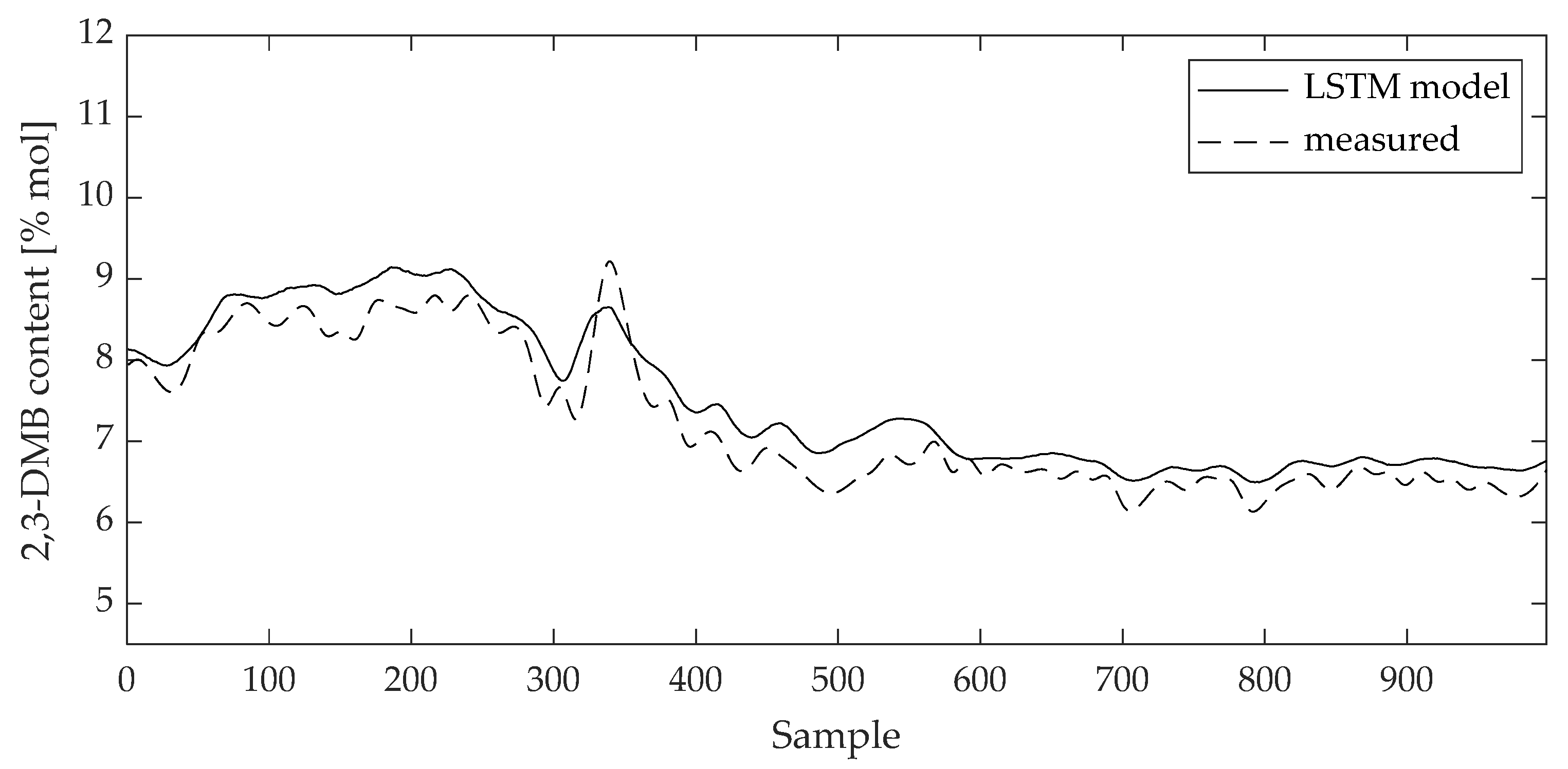
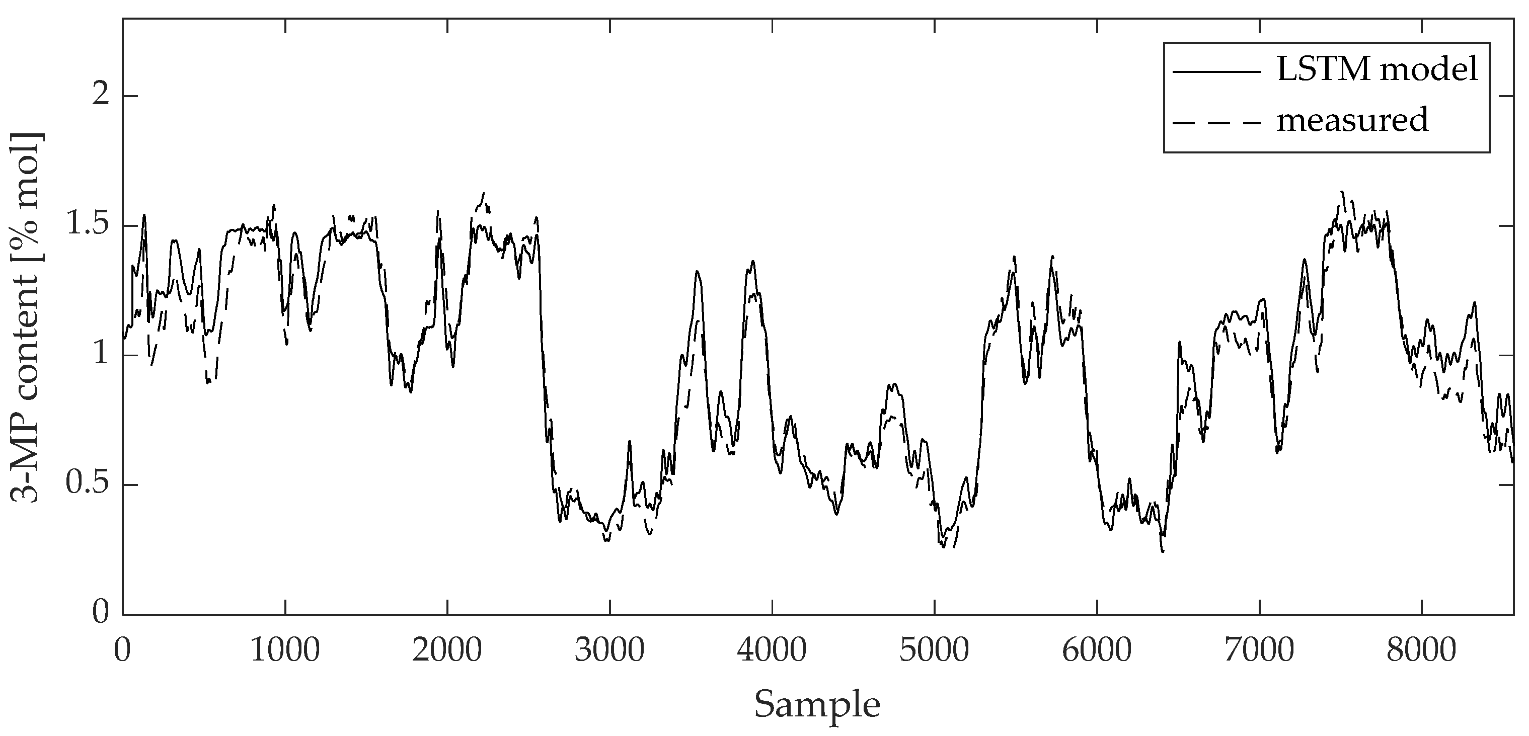
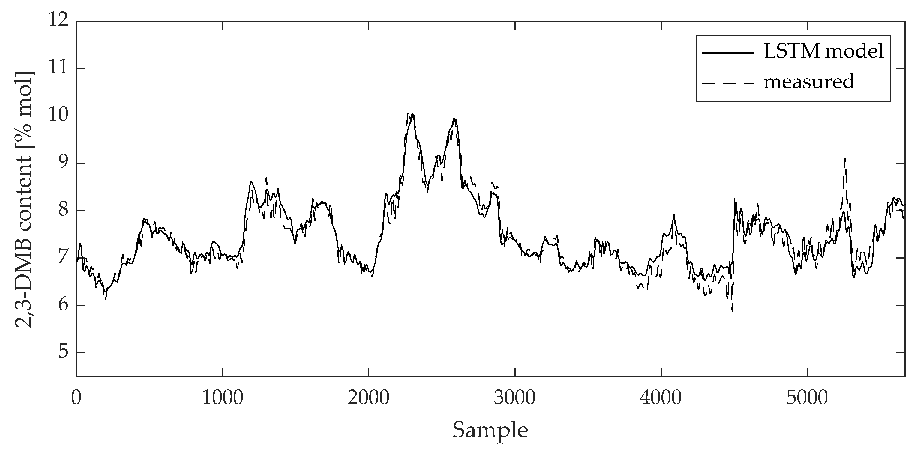
3. Results
4. Discussion
5. Conclusions
Author Contributions
Funding
Data Availability Statement
Conflicts of Interest
References
- Han, Y.; Huang, G.; Song, S.; Yang, L.; Wang, H.; Wang, Y. Dynamic Neural Networks: A Survey. IEEE Trans. Pattern Anal. Mach. Intell. 2022, 44, 7436–7456. [Google Scholar] [CrossRef] [PubMed]
- Medsker, L.R.; Jain, L.C. (Eds.) Recurrent Neural Networks Design and Applications; CRC Press: Boca Raton, FL, USA, 2001. [Google Scholar]
- Gillioz, A.; Casas, J.; Mugellini, E.; Khaled, O.A. Overview of the Transformer-based Models for NLP Tasks. In Proceedings of the 2020 15th Conference on Computer Science and Information Systems (FedCSIS), Sofia, Bulgaria, 6–9 September 2020. [Google Scholar] [CrossRef]
- Wan, R.; Mei, S.; Wang, J.; Liu, M.; Yang, F. Multivariate Temporal Convolutional Network: A Deep Neural Networks Approach for Multivariate Time Series Forecasting. Electronics 2019, 8, 876. [Google Scholar] [CrossRef]
- Yao, X.; Shao, Y.; Fan, S.; Cao, S. Echo state network with multiple delayed outputs for multiple delayed time series prediction. J. Frank. Inst. 2022, 359, 11089–11107. [Google Scholar] [CrossRef]
- Faradonbe, S.M.; Safi-Esfahani, F.; Karimian-Kelishadrokhi, M. A Review on Neural Turing Machine (NMT). SN Comput. Sci. 2020, 1, 333. [Google Scholar] [CrossRef]
- Rakhmatullin, A.K.; Gibadullin, R.F. Synthesis and Analysis of Elementary Algorithms for a Differential Neural Computer. Lobachevskii J. Math. 2022, 43, 473–483. [Google Scholar] [CrossRef]
- Soydaner, D. Attention mechanism in neural networks: Where it comes and where it goes. Neural Comput. Appl. 2022, 34, 13371–13385. [Google Scholar] [CrossRef]
- Widrow, B.; Winter, R. Neural nets for adaptive filtering and adaptive pattern recognitions. Computer 1988, 21, 25–39. [Google Scholar] [CrossRef]
- Rao, A.R.; Reimherr, M. Nonlinear Functional Modeling Using Neural Networks. J. Comput. Graph. Stat. 2023, 1–10. [Google Scholar] [CrossRef]
- Graves, A. Supervised Sequence Labelling with Reccurent Neural Networks; Springer: New York, NY, USA, 2012. [Google Scholar]
- Hochreiter, S.; Schmidhuber, J. Long Short-Term Memory. Neural Comput. 1997, 9, 1735–1780. [Google Scholar] [CrossRef]
- Van Houdt, G.; Mosquera, C.; Nápoles, G. A review on the long short-term memory model. Artif. Intell. Rev. 2020, 53, 5929–5955. [Google Scholar] [CrossRef]
- Liu, Y.; Young, R.; Jafarpour, B. Long–short-term memory encoder–decoder with regularized hidden dynamics for fault detection in industrial processes. J. Process Control 2023, 124, 166–178. [Google Scholar] [CrossRef]
- Aghaee, M.; Krau, S.; Tamer, M.; Budman, H. Unsupervised Fault Detection of Pharmaceutical Processes Using Long Short-Term Memory Autoencoders. Ind. Eng. Chem. Res. 2023, 62, 9773–9786. [Google Scholar] [CrossRef]
- Yao, P.; Yang, S.; Li, P. Fault Diagnosis Based on RseNet-LSTM for Industrial Process. In Proceedings of the 2021 IEEE 5th Advanced Information Technology, Electronic and Automation Control Conference (IAEAC), Chongqing, China, 12–14 March 2021. [Google Scholar]
- Zhang, H.; Niu, G.; Zhang, B.; Miao, Q. Cost-Effective Lebesgue Sampling Long Short-Term Memory Networks for Lithium-Ion Batteries Diagnosis and Prognosis. IEEE Trans. Ind. Electron. 2021, 69, 1958–1964. [Google Scholar] [CrossRef]
- He, R.; Chen, G.; Sun, S.; Dong, C.; Jiang, S. Attention-Based Long Short-Term Memory Method for Alarm Root-Cause Diagnosis in Chemical Processes. Ind. Eng. Chem. Res. 2020, 59, 11559–11569. [Google Scholar] [CrossRef]
- Yu, J.; Liu, X.; Ye, L. Convolutional Long Short-Term Memory Autoencoder-Based Feature Learning for Fault Detection in Industrial Processes. IEEE Trans. Instrum. Meas. 2020, 70, 3505615. [Google Scholar] [CrossRef]
- Tan, Q.; Li, B. Soft Sensor Modeling Method for Sulfur Recovery Process Based on Long Short-Term Memory Artificial Neural Network (LSTM). In Proceedings of the 2023 9th International Conference on Energy Materials and Environment Engineering (ICEMEE 2023), Kuala Lumpur, Malaysia, 8–10 June 2023. [Google Scholar]
- Curreri, F.; Patanè, L.; Xibilia, M.G. RNN- and LSTM-Based Soft Sensors Transferability for an Industrial Process. Sensors 2021, 21, 823. [Google Scholar] [CrossRef]
- Yuan, X.; Li, L.; Wang, Y. Nonlinear Dynamic Soft Sensor Modeling With Supervised Long Short-Term Memory Network. IEEE Trans. Ind. Inform. 2020, 16, 3168–3176. [Google Scholar] [CrossRef]
- Liu, Q.; Jia, M.; Gao, Z.; Xu, L.; Liu, Y. Correntropy long short term memory soft sensor for quality prediction in industrial polyethylene process. Chemom. Intell. Lab. Syst. 2022, 231, 104678. [Google Scholar] [CrossRef]
- Zhou, J.; Wang, X.; Yang, C.; Xiong, W. A Novel Soft Sensor Modeling Approach Based on Difference-LSTM for Complex Industrial Process. IEEE Trans. Ind. Inform. 2022, 18, 2955–2964. [Google Scholar] [CrossRef]
- Geng, Z.; Chen, Z.; Meng, Q.; Han, Y. Novel Transformer Based on Gated Convolutional Neural Network for Dynamic Soft Sensor Modeling of Industrial Processes. IEEE Trans. Ind. Inform. 2022, 18, 1521–1529. [Google Scholar] [CrossRef]
- Feng, Z.; Li, Y.; Sun, B. A multimode mechanism-guided product quality estimation approach for multi-rate industrial processes. Inf. Sci. 2022, 596, 489–500. [Google Scholar] [CrossRef]
- Sun, M.; Zhang, Z.; Zhou, Y.; Xia, Z.; Zhou, Z.; Zhang, L. Convolution and Long Short-Term Memory Neural Network for PECVD Process Quality Prediction. In Proceedings of the 2021 Global Reliability and Prognostics and Health Management (PHM-Nanjing), Nanjing, China, 15–17 October 2021. [Google Scholar]
- Tang, Y.; Wang, Y.; Liu, C.; Yuan, X.; Wang, K.; Yang, C. Semi-supervised LSTM with historical feature fusion attention for temporal sequence dynamic modeling in industrial processes. Eng. Appl. Artif. Intell. 2023, 117, 105547. [Google Scholar] [CrossRef]
- Lei, R.; Guo, Y.B.; Guo, W. Physics-guided long short-term memory networks for emission prediction in laser powder bed fusion. J. Manuf. Sci. Eng. 2023, 146, 011006. [Google Scholar] [CrossRef]
- Jin, N.; Zeng, Y.; Yan, K.; Ji, Z. Multivariate Air Quality Forecasting With Nested Long Short Term Memory Neural Network. IEEE Trans. Ind. Inform. 2021, 17, 8514–8522. [Google Scholar] [CrossRef]
- Xu, B.; Pooi, C.K.; Tan, K.M.; Huang, S.; Shi, X.; Ng, H.Y. A novel long short-term memory artificial neural network (LSTM)-based soft-sensor to monitor and forecast wastewater treatment performance. J. Water Process Eng. 2023, 54, 104041. [Google Scholar] [CrossRef]
- Wang, T.; Leung, H.; Zhao, J.; Wang, W. Multiseries Featural LSTM for Partial Periodic Time-Series Prediction: A Case Study for Steel Industry. IEEE Trans. Instrum. Meas. 2020, 69, 5994–6003. [Google Scholar] [CrossRef]
- Mateus, B.C.; Mendes, M.; Farinha, J.T.; Cardoso, A.M. Anticipating Future Behavior of an Industrial Press Using LSTM Networks. Appl. Sci. 2021, 11, 6101. [Google Scholar] [CrossRef]
- Kazi, M.K.; Eljack, F. Practicality of Green H2 Economy for Industry and Maritime Sector Decarbonization through Multiobjective Optimization and RNN-LSTM Model Analysis. Ind. Eng. Chem. Res. 2022, 61, 6173–6189. [Google Scholar] [CrossRef]
- Ma, S.; Zhang, Y.; Lv, J.; Ge, Y.; Yang, H.; Li, L. Big data driven predictive production planning for energy-intensive manufacturing industries. Energy 2020, 211, 118320. [Google Scholar] [CrossRef]
- Hamied, R.S.; Shakor, Z.M.; Sadeiq, A.H.; Abdul Razak, A.A.; Khadim, A.T. Kinetic Modeling of Light Naphtha Hydroisomerization in an Industrial Universal Oil Products Penex™ Unit. Energy Eng. 2023, 120, 1371–1386. [Google Scholar] [CrossRef]
- Khajah, M.; Chehadeh, D. Modeling and active constrained optimization of C5/C6 isomerization via Artificial Neural Networks. Chem. Eng. Res. Des. 2022, 182, 395–409. [Google Scholar] [CrossRef]
- Abdolkarimi, V.; Sari, A.; Shokri, S. Robust prediction and optimization of gasoline quality using data-driven adaptive modeling for a light naphtha isomerization reactor. Fuel 2022, 328, 125304. [Google Scholar] [CrossRef]
- Lukec, I.; Lukec, D.; Sertić Bionda, K.; Adžamić, Z. The possibilities of advancing isomerization process through continuous optimization. Goriva I Maz. 2007, 46, 234–245. [Google Scholar]
- Ujević Andrijić, Ž.; Herceg, S.; Bolf, N. Data-driven estimation of critical quality attributes on industrial processes. In Proceedings of the 19th Ružička Days “Today Science—Tomorrow Industry” international conference, Vukovar, Croatia, 21–23 September 2022. [Google Scholar]
- Herceg, S.; Ujević Andrijić, Ž.; Bolf, N. Support vector machine-based soft sensors in the isomerization process. Chem. Biochem. Eng. Q. 2020, 34, 243–255. [Google Scholar] [CrossRef]
- Herceg, S.; Ujević Andrijić, Ž.; Bolf, N. Development of soft sensors for isomerization process based on support vector machine regression and dynamic polynomial models. Chem. Eng. Res. Des. 2019, 149, 95–103. [Google Scholar] [CrossRef]
- Herceg, S.; Ujević Andrijić, Ž.; Bolf, N. Continuous estimation of the key components content in the isomerization process products. Chem. Eng. Trans. 2018, 69, 79–84. [Google Scholar] [CrossRef]
- Fortuna, L.; Graziani, S.; Rizzo, A.; Xibilia, M.G. Soft Sensors for Monitoring and Control of Industrial Processes (Advances in Industrial Control); Springer: London, UK, 2007. [Google Scholar]
- Kadlec, P.; Gabrys, B.; Strandt, S. Data-driven Soft Sensors in the process industry. Comput. Chem. Eng. 2009, 33, 795–814. [Google Scholar] [CrossRef]
- Greff, K.; Srivastava, R.K.; Koutník, J.; Steunebrink, B.R.; Schmidhuber, J. LSTM: A Search Space Odyssey. IEEE Trans. Neural Netw. Learn. Syst. 2017, 28, 2222–2232. [Google Scholar] [CrossRef]
- Beale, M.H.; Hagan, M.T.; Demuth, H.B. Deep Learning Toolbox™ User’s Guide; The MathWorks, Inc.: Natick, MA, USA, 2020; pp. 53–64. [Google Scholar]
- Goodfellow, I.; Bengio, Y.; Courville, A. Deep Learning; The MIT Press: Cambridge, MA, USA, 2016; pp. 267–320. [Google Scholar]
- Cusher, N.A. UOP Penex Process. In Handbook of Petroleum Refining Processes, 3rd ed.; Meyers, R.A., Ed.; McGraw-Hill: New York, NY, USA, 2003; pp. 9.15–9.27. [Google Scholar]
- Cerić, E. Nafta, Procesi i Proizvodi; IBC d.o.o.: Sarajevo, Bosnia and Herzegovina, 2012. [Google Scholar]
- Herceg, S. Development of Soft Sensors for Advanced Control of Isomerization Process. Doctoral Thesis, University of Zagreb, Zagreb, Croatia, 30 September 2021. [Google Scholar]


| Variable | Tag | Unit |
|---|---|---|
| DIH column overhead vapor temperature | TI-046 | °C |
| 21st DIH column tray temperature | TIC-047 | °C |
| DIH column side product temperature | TI-045 | °C |
| DIH column bottom product temperature | TI-049 | °C |
| DIH column reflux | FI-028 | m3/h |
| DIH column reflux flow and isomerate flow sum | FIC-029 | m3/h |
| DIH column bottom product flow | FIC-026 | m3/h |
| DIH column side product flow | FIC-020 | m3/h |
| Feature | Training Data Set | Test Data Set |
|---|---|---|
| Learning algorithm | ADAM | ADAM |
| Activation function | tanh | tanh |
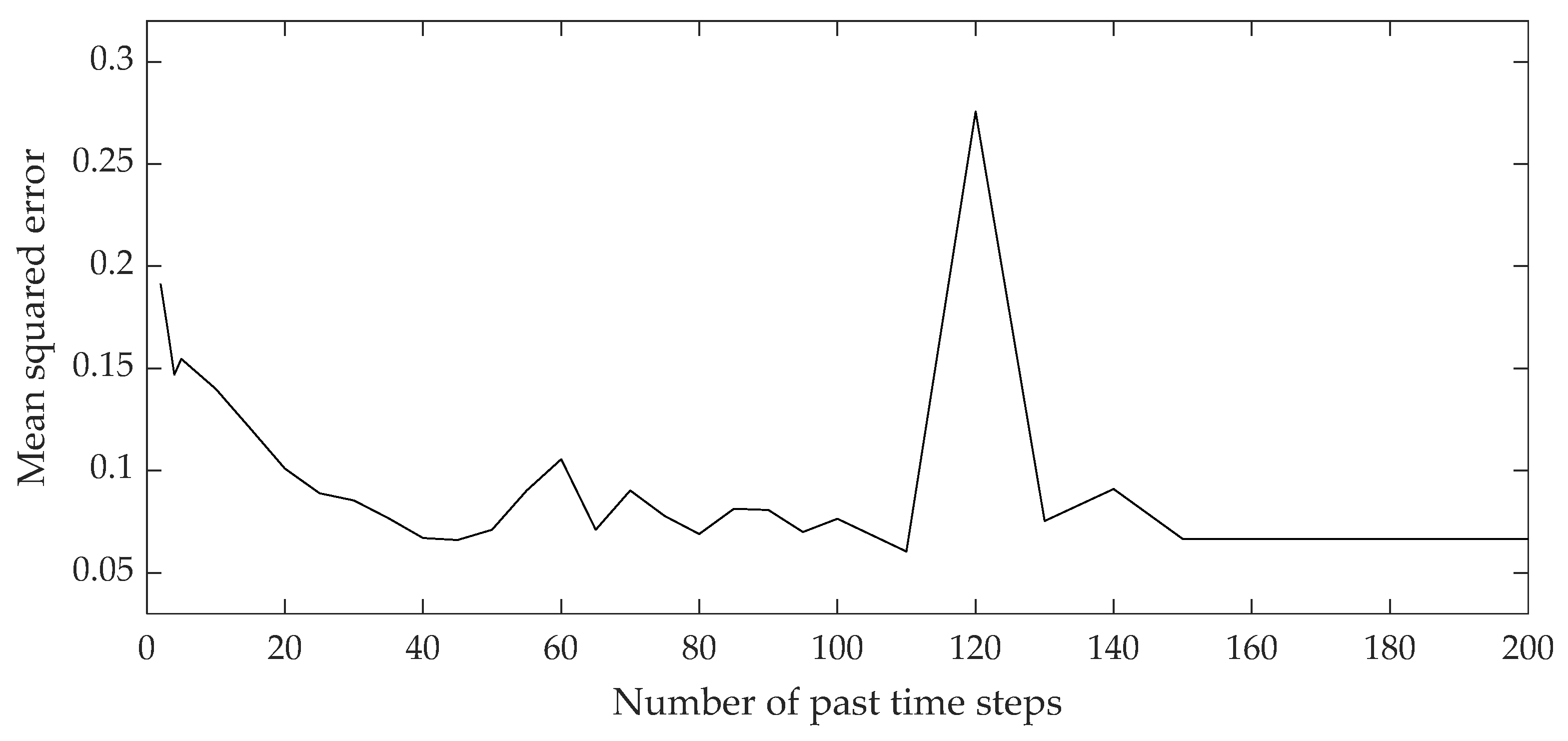
| Number of past time steps | 45 | 45 |
| Number of hidden units | 25 | 25 |
| R | 0.963 | 0.978 |
| 0.924 | 0.865 | |
| RMSE [% mol] | 0.207 | 0.326 |
| MAE [% mol] | 0.155 | 0.284 |
| Feature | Training Data Set | Test Data Set |
|---|---|---|
| Learning algorithm | ADAM | ADAM |
| Activation function | tanh | tanh |
| Number of past time steps | 55 | 55 |
| Number of hidden units | 25 | 25 |
| R | 0.972 | 0.988 |
| 0.945 | 0.973 | |
| RMSE [% mol] | 0.089 | 0.048 |
| MAE [% mol] | 0.071 | 0.037 |
| Model | R (Test) | R2 (Test) | RMSE (Test) [% mol] | MAE (Test) [% mol] |
|---|---|---|---|---|
| LSTM | 0.978 | 0.865 | 0.326 | 0.284 |
| MLP 7-15-1 [35] | 0.974 | 0.949 | 0.179 | 0.141 |
| SVM [36] | 0.988 | 0.977 | 0.118 | 0.077 |
| FIR [38] | 0.948 | 0.878 | 0.266 | 0.213 |
| ARX [38] | 0.963 | 0.925 | 0.209 | 0.163 |
| OE [38] | 0.965 | 0.928 | 0.204 | 0.152 |
| NARX [38] | 0.965 | 0.927 | 0.206 | 0.163 |
| HW [38] | 0.967 | 0.934 | 0.196 | 0.149 |
| Model | R (Test) | R2 (Test) | RMSE (Test) [% mol] | MAE (Test) [% mol] |
|---|---|---|---|---|
| LSTM | 0.988 | 0.973 | 0.048 | 0.037 |
| MLP 6-20-1 | 0.968 | 0.936 | 0.091 | 0.067 |
| SVM [37] | 0.982 | 0.965 | 0.069 | 0.045 |
| FIR [37] | 0.942 | 0.883 | 0.105 | 0.083 |
| ARX [37] | 0.983 | 0.965 | 0.058 | 0.049 |
| OE [37] | 0.989 | 0.977 | 0.046 | 0.037 |
| NARX [37] | 0.985 | 0.969 | 0.054 | 0.046 |
| HW [37] | 0.995 | 0.989 | 0.033 | 0.026 |
| Variable | Samples | Mean | Median | Min | Max | Variance | Std. Dev. |
|---|---|---|---|---|---|---|---|
| TI-046 | 6667 | 75.43 | 75.72 | 72.54 | 77.57 | 1.083 | 1.041 |
| TIC-047 | 6667 | 87.29 | 87.65 | 82.55 | 88.40 | 1.072 | 1.035 |
| TI-045 | 6667 | 97.23 | 97.26 | 96.19 | 98.19 | 0.072 | 0.268 |
| TI-049 | 6667 | 121.7 | 121.8 | 117.4 | 125.0 | 1.078 | 1.038 |
| FI-028 | 6667 | 378.2 | 377.4 | 360.8 | 397.5 | 38.22 | 6.182 |
| FIC-029 | 6667 | 426.2 | 426.5 | 404.7 | 448.9 | 29.69 | 5.448 |
| FIC-026 | 6667 | 5.534 | 5.497 | 2.966 | 11.00 | 1.826 | 1.351 |
| AI-004B | 6667 | 7.417 | 7.278 | 5.871 | 10.12 | 0.605 | 0.778 |
| Variable | Samples | Mean | Median | Min | Max | Variance | Std. Dev. |
|---|---|---|---|---|---|---|---|
| TI-046 | 10,078 | 75.93 | 75.99 | 73.44 | 77.89 | 0.804 | 0.897 |
| TIC-047 | 10,078 | 87.67 | 87.76 | 86.26 | 88.65 | 0.175 | 0.418 |
| TI-045 | 10,078 | 97.15 | 97.16 | 96.21 | 97.89 | 0.060 | 0.245 |
| TI-049 | 10,078 | 122.7 | 122.8 | 119.6 | 125.3 | 1.004 | 1.002 |
| FI-028 | 10,078 | 372.4 | 372.2 | 357.1 | 386.7 | 36.67 | 6.056 |
| FIC-029 | 10,078 | 422.3 | 422.6 | 404.7 | 439.0 | 18.19 | 4.265 |
| AIC-005A | 10,078 | 0.924 | 0.975 | 0.241 | 1.632 | 0.135 | 0.368 |
Disclaimer/Publisher’s Note: The statements, opinions and data contained in all publications are solely those of the individual author(s) and contributor(s) and not of MDPI and/or the editor(s). MDPI and/or the editor(s) disclaim responsibility for any injury to people or property resulting from any ideas, methods, instructions or products referred to in the content. |
© 2023 by the authors. Licensee MDPI, Basel, Switzerland. This article is an open access article distributed under the terms and conditions of the Creative Commons Attribution (CC BY) license (https://creativecommons.org/licenses/by/4.0/).
Share and Cite
Herceg, S.; Ujević Andrijić, Ž.; Rimac, N.; Bolf, N. Development of Mathematical Models for Industrial Processes Using Dynamic Neural Networks. Mathematics 2023, 11, 4518. https://doi.org/10.3390/math11214518
Herceg S, Ujević Andrijić Ž, Rimac N, Bolf N. Development of Mathematical Models for Industrial Processes Using Dynamic Neural Networks. Mathematics. 2023; 11(21):4518. https://doi.org/10.3390/math11214518
Chicago/Turabian StyleHerceg, Srečko, Željka Ujević Andrijić, Nikola Rimac, and Nenad Bolf. 2023. "Development of Mathematical Models for Industrial Processes Using Dynamic Neural Networks" Mathematics 11, no. 21: 4518. https://doi.org/10.3390/math11214518
APA StyleHerceg, S., Ujević Andrijić, Ž., Rimac, N., & Bolf, N. (2023). Development of Mathematical Models for Industrial Processes Using Dynamic Neural Networks. Mathematics, 11(21), 4518. https://doi.org/10.3390/math11214518