Peculiarity of Behavior of Economic Agents under Cognitive Constraints in a Semi-Open New Keynesian Model

Abstract

The aim of the paper is to analyze changes and peculiarities of behavior of economic agents with bounded rationality in the New Keynesian model, in which imported equipment and technology are one of the factors of production, and households consume only domestic products. The formation of output gap and inflation expectations by agents is based on stationary values of these variables and on extrapolation of the latest available data on inflation and the output gap. The weight shares of agents applying these rules change endogenously. Histograms of the frequency distribution of the degree of buoyancy and the impulse responses of monetary policy shocks and technology shocks to the variables under study show that a less open economy tends to go through an economic cycle with a smaller amplitude than a more rigid economy. Analyses of the trade-offs between the volatility of inflation and the output gap at different parameter values in the Taylor rule show their non-linear nature (in contrast to standard models with rational expectations). An important result obtained in this analysis is that the rational expectations hypothesis is more consistent with a closed economy than with an open one.

1. Introduction

In recent decades, theoretical contributions to macroeconomics have largely been based on dynamic stochastic general equilibrium models (DSGE models) with rational expectations, in which a representative agent is able to understand the complexity of the underlying mathematical model [1,2]. The advantage of these models is, firstly, that they have microeconomic justifications. It is assumed that consumers maximize the expected discounted sum of utility function values and produce their profits over time. This implies that macroeconomic equations must be derived from this optimizing behavior of consumers and producers.

Secondly, it is assumed that consumers and producers have rational expectations, i.e., make predictions using all available information, including information embedded in the model [3,4,5]. This assumption also means that agents know the true statistical distribution of all shocks hitting the economy. They then use this information in their optimization procedure. Since consumers and all producers use the same information, we can take only one representative of the consumer and producer to model the entire economy. There is no heterogeneity in the behavior of consumers and producers.

Third, and this is a new Keynesian feature, it is assumed that prices are not set instantaneously. This feature contrasts with the real business cycle model, which assumes perfect price flexibility.

However, the global financial crisis has shown that agents do not fully understand the complexity of the world in which they live. On the contrary, their cognitive capabilities seem to be quite limited. Numerous data and evidence indicate the importance of including heterogeneous expectations in general equilibrium models [6,7,8,9,10].

It should be noted that a stylized DSGE rational expectations model cannot capture the typical features of real business cycle movement, that is, the correlation between subsequent observations of the output gap (autocorrelation) and the occurrence of large booms and busts (fat tails of variable distributions) without incorporating less than reasonable assumptions. Therefore, it is necessary to develop macroeconomic models that do not impose the implausible cognitive abilities of individual agents.

In addition, under uncertainty, the idea of “rational behavior” cannot be allowed, as risk aversion prevails in the agents’ behavior, which contradicts the neoclassical assumption that the representative agent of the model always maximizes profit or utility. This is because uncertainty increases with shocks to macroeconomic variables, and such shocks are very frequent in today’s global world. If a DSGE model always moves towards equilibrium, it is because it was constructed that way, not because it is a good interpretation of the real world.

Standard DSGE models are not intended for their use in describing extreme events because they deal with low-intensity shocks rather than shocks that increase uncertainty. It should be noted that a stylized DSGE model with rational expectations cannot capture the typical features of real business cycle movements, i.e., the correlation between subsequent observations of the output gap (autocorrelation) and the occurrence of large rises and falls (thick tails of variable distributions) without incorporating assumptions that are not entirely reasonable.

Thus, based on the above, there is a need to develop macroeconomic models that do not impose implausible cognitive abilities on individual agents.

Under special conditions, such as during the sanctions period, there are problems with the supply and use of imported equipment and technologies in the real sector of the economy. At the moment, China and other Asian countries are helping the Russian economy with these supplies. Therefore, it is of interest to study a model in which the import component is, along with labor, a factor of production. At the same time, households, due to sanctions, consume only domestically produced goods and products. The New Keynesian model can be the basis for such a model [11]. Unlike the cited work, in which agents make forecasts based on rational expectations, in the work under study, economic agents have bounded rationality, which is natural during the sanctions period with turbulent processes in the economy.

The formation of expectations in New Keynesian models is realized by means of certain rules for agents forecasting the output gap and price inflation. In this context, the output gap is a summary indicator of the relative relationship between the demand and supply components of economic activity. In essence, the output gap measures the degree of inflationary pressure in the economy and is an important link between the real part of the economy that produces goods and services and inflation.

Based on the above, the purpose and scientific novelty of the paper is to analyze the changes and characteristics of the economic agent’s behavior when including heterogeneous expectations in the new Keynesian model based on the model [11]. The objectives of the study are to analyze the histograms of the frequency distribution of the degree of vital forces and impulse response functions of closed and more open economy models, as well as to analyze the trade-offs between the volatility of inflation and the output gap at different values of parameters in the Taylor rule in these models. The formation of expectations in the model under study is viewed as an interactive process between fundamentalist agents forecasting the output gap and price inflation on the basis of their stationary values and agents using a forecasting rule based on extrapolation of the latest available data on inflation and the output gap.

This paper is structured as follows. Section 2 provides a review of the literature on the topic under study. Section 3 describes the model and the mechanism of formation of expectations of economic agents. Section 4 and Section 5 summarize the results of the study and their discussion. Finally, the conclusion (Section 6) summarizes the results of the study.

2. Literature Review

It should be noted that empirical evidence of the heterogeneity of agents and their limited cognitive abilities has been provided using both laboratory data and survey data [12,13,14,15,16]. Researchers have only recently begun to incorporate elements of behavioral economics into dynamic macromodels [17,18,19,20]. In addition, some publications highlight that the linearity implied by standard rational expectations DSGE models makes them not fully suitable for monetary and fiscal policy analysis. The use of macroeconomic models that take into account the cognitive limitations of agents can improve understanding of the behavior of economic agents in the real world. For example, dynamic macroeconomic models are analyzed under the assumption that agents have bounded rationality and form their expectations based on simple heuristics in the works [21,22,23]. Two types of agents are considered. The first type of agent predicts the output gap and inflation based on their stationary values. In what follows, these agents will be called fundamentalist agents. The second type of agent uses a simple forecasting rule based on extrapolation of the latest available data on inflation and the output gap. In the future, these agents will be called extrapolating agents. DeGrauwe [22] implements these heterogeneous expectations in a standard three-equation sticky-price New Keynesian model and shows how such a structure can generate endogenous waves of agents’ optimistic and pessimistic beliefs (animal spirits), which are closely associated with the business cycle. At the same time, in the models under study, agents are ready to learn; that is, they constantly evaluate the effectiveness of their forecast. This willingness to learn and change one’s behavior is the fundamental definition of rational behavior. Thus, the analyzed agents in the studied models are rational, but not in the sense that they have rational expectations. Instead, agents are rational in the sense that they learn from their mistakes. To characterize such behavior, the concept of “bounded rationality” is often used, which will be used in the following discussion.

The behavioral model [24] shows that differences in attitudes combined with borrowing constraints tend to restrain economic growth but generate a chain reaction that exacerbates recessions. The model is an example of endogenous credit cycles with expansions, severe recessions, and persistent wealth inequality. The model [25] analyses fiscal consolidation using a New Keynesian model in which agents have heterogeneous expectations. The authors consider expenditure-based and tax-based consolidation, and their effects are analyzed separately. Consolidation effects and output multipliers are found to be sensitive to heterogeneity of expectations before and after the implementation of a particular fiscal plan. Depending on the perceptions of the type of consolidation before its implementation, it is shown that heterogeneity of expectations can lead to optimism in the economy, thus improving the implementation of a specific fiscal plan, or it can work in the opposite direction, leading to pessimism and increasing the constraining effect of consolidation.

Additionally, agents can use simpler rules (heuristics) to predict future output and inflation. It is assumed that because agents do not fully understand how the output gap and inflation are determined, their forecasts are biased. It is believed that some agents are optimistic and systematically increase the output gap and inflation, while others are pessimistic and systematically underestimate these variables.

The papers [26,27,28] introduce a selection mechanism that disciplines agents to choose appropriate heuristics from a set of rules according to a suitability criterion. This allows agents to learn from past mistakes and select heuristics that have performed well in the (recent) past.

In the vast majority of publications (including those listed above) analyzing agents’ cognitive constraints, labor is the only factor of production. At the same time, during the period of sanctions, the real sector of the sanctioned economy is in dire need of supplies and use of imported equipment and technologies, while households consume only domestic goods. Therefore, the import component as a factor of production should be present in the models describing such an economy. The authors know of only one similar work [11], in which agents make forecasts using rational expectations. However, the sanctions period is characterized by uncertainty, and therefore, it is of interest to consider the model [11] from the standpoint of the bounded rationality of agents.

The distribution of agent heterogeneity changes over time, which is confirmed by many empirical data. For example, in the work by [29], various studies of inflation expectations show a wide, time-varying range of opinions. Works by [14,30] confirm the time-varying distribution of agents with discrete (exogenous) predictors. The proposed paper is an extension of the last listed publications, in which the ratio of fundamentalists agents and extrapolators agents, by analogy with the work [31], is endogenous. This article also expands the publications [21,22,23], including the endogenous selection of predictors in the New Keynesian model with the import component as a factor of production.

In addition to those papers described above, noteworthy is the approach based on the dynamics of agent learning in macroeconomic models, first proposed by Sargent [32] and Evans, Honkapohja [33]. This approach leads to new important conclusions [34,35,36]. For example, in the work by [36], evaluation results show that private agents often switched to constant reinforcement learning during most of the 1970s and until the early 1980s and later reduced learning efforts. As a result, the model can generate volatility that increases in the 1970s and then falls in a period that could roughly match the magnitude of the so-called “Great Slowdown” of 1984–2007. One of the options for dynamic agent training is an approach based on adaptive agent learning [37]. The authors of this approach found that irrational beliefs of agents based on small forecasting models are more closely related to survey data on inflation expectations than beliefs based on rational expectations. However, as De Grauwe [22] points out, the above approaches place too many cognitive constraints on agents that they probably do not possess in the real world.

In addition to those described above, it is worth noting the approaches to modeling the behavior of economic agents that are not related to the optimization of firms’ profits or utility of consumption, for example, the agent-based approach [38,39,40]. In particular, [41] analyzed the effects of Brexit on UK and EU banks using this approach. The results suggest that policymakers should take into account the dynamic effects that may be caused by UK banks moving to the EU after Brexit. With such a move of UK banks to the EU, the negative effects in the EU from Brexit would be mitigated.

Scenario approaches are also interesting in this context. For example, in [42], simulations conducted using a low-dimensional macro-econometric model and various scenarios showed that in Greece, while dealing with a very high public debt-to-GDP ratio, no real policy would be effective. Austerity measures, although severe, will not bring the debt below 100% in the near- and medium-term future. This result is very important and of great significance for the future of Europe and the prevention of a Eurozone crisis.

It should be noted that the vast majority of New Keynesian models that study the behavior of agents with bounded rational expectations are models with rigid prices. However, the factor for justification of unforeseen behavior of economic agents can also be rigid wages. In this regard, the authors’ work [43], which shows the change in the behavior of agents when introducing this type of market imperfections into the model, is interesting.

Thus, it follows from the above literature review that the analysis of the behavior of economic agents in models with boundedly rational expectations is relevant and requires further study and testing on various models. Including models in which the import component is a factor of production. The present study is devoted to such an analysis of the behavior of economic agents in such a model.

3. Materials and Methods

3.1. Description of the Model

The model under study is a new Keynesian model in which nominal prices are rigid. A detailed description of the model is presented in the work [11]. The main assumptions of the model are as follows.

All model equations are given in log linearized form. Euler’s equation is obtained when households choose the optimal trajectory of consumption and asset holdings. The aggregate Euler equation (Logarithm of the consumer aggregate $c_t=\ln C_t,$ where $C_t={\left[{\displaystyle \underset{0}{\overset{1}{\int }}{C}_t{(i)}^{({\epsilon }_p-1)/{\epsilon }_p}}\right]}^{\frac{{\epsilon }_p}{({\epsilon }_p-1)}}$, where $i$- index of differentiated goods, $i\in [01]$, ${\epsilon }_p$—elasticity of substitution between these goods. Corresponding price index $P_t={\left[{\displaystyle \underset{0}{\overset{1}{\int }}{P}_t{(i)}^{(1-{\epsilon }_p)}}\right]}^{\frac{1}{(1-{\epsilon }_p)}}$). (in general equilibrium) for households, obtained from first-order conditions, is

$$\begin{array}{c}{c}_t={\tilde{E}}_t{c}_{t+1}-b_1(R_t-{\tilde{E}}_t{\pi }_{t+1})+{\mu }_t,\\ {\mu }_t~N(0,{\sigma }_u^2),\end{array}$$

(1)

where ${\tilde{E}}_t$ is the operator characterizing the bounded rationality of agents, $R_t$ is the nominal interest rate, ${\pi }_t$—price inflation, ${\mu }_t$—consumption shock (taste shock), and the parameter $b_1$ characterizes the elasticity of intertemporal substitution.

Firms produce differentiated products according to the production function as follows:

$$y_t=(1-\alpha )(n_t+a_t)+\alpha im{p}_t$$

(2)

where $y_t$ the volume of output $\alpha$ is the share of the imported component in production, $a_t$—labor productivity, changing in accordance with the autoregressive law (AR1) and characterizing labor-saving progress.

Minimizing the costs associated with import demand leads to the equation:

$$imp=y_t-\sigma s_t$$

(3)

where $\sigma$ is the elasticity of substitution between labor and the import component of domestic production, $s_t$—the real exchange rate

$$s_t=e_t-p_t+p_t^{*},$$

(4)

where $e_t$ is the nominal exchange rate of the currencies of the two countries, $p_t,p_t^{*}$ are the consumer price indices. (In what follows, all variables with asterisks refer to the foreign economy).

Similar to Equation (3), export demand is determined by

$$\exp =y_t^{*}+{\sigma }^{*}{s}_t,$$

(5)

where $y_t^{*},$ ${\sigma }^{*}$ is the volume of output and the elasticity of substitution between labor and imports in a foreign economy.

The equation for uncovered interest rate parity is:

$$R_t=R_t^{*}+{\tilde{E}}_t{e}_{t+1}-e_t.$$

(6)

The resource limitation for the model under study has the following form:

$$y_t={\omega }_1{c}_t+{\omega }_2{g}_t+{\omega }_3\exp$$

(7)

where $g_t$ is the government spending, changing in accordance with the autoregressive law (AR 1), ${\omega }_1,{\omega }_2,{\omega }_3$ is the stationary value of the ratio of the corresponding variables to the volume of output.

Firms set prices in accordance with the Calvo approach [44,45]. Some firms (1 − ${\theta }_p$) revise prices $P_t^{onm}$ in each period; the other part ${\theta }_p$, which does not change prices, indexes them in each period. The pricing problem for a firm that gets the opportunity to update its price in period t is dynamic: the price it chooses today will affect the profits it earns both today and in the future. A firm that adjusts its price in period t solves the problem of optimizing profits while limiting demand for products:

$$Y_{t+k,t}={\left(\frac{P_t^{onm}}{P_{t+k}}\right)}^{-{\epsilon }_p}{C}_{t+k},$$

(8)

for k = 0, 1, 2, …, where $Y_{t+k,t}$ is the volume of production in period t + k by firms that adjusted their price last time in period t, $C_{t+k}$ is the volume of consumption in period t + k, ${\epsilon }_p$—the elasticity of substitution of differentiated goods.

Solving the optimization problem for firms leads to the Phillips curve equation

$$\begin{array}{c}{\pi }_t=\beta {\tilde{E}}_t{\pi }_{t+1}+{\kappa }_p{x}_t+u_t,\\ u_t~N(0,{\sigma }_u^2),\\ {\kappa }_p=\frac{\alpha {\lambda }_p}{1-\alpha },\\ {\lambda }_p=\frac{(1-{\theta }_p)(1-\beta {\theta }_p)}{{\theta }_p}\frac{1-\alpha }{1-\alpha +\alpha {\epsilon }_p}\end{array}$$

(9)

where $x_t$ is the output gap between the actual and stationary value. $u_t$—cost shock, ${\kappa }_p$, ${\lambda }_p$, ${\epsilon }_p$ is the elasticity of substitution of differentiated goods produced by firms.

Equation (10) for the nominal interest rate $R_t$ (Taylor’s rule) closes the system.

$$\begin{array}{c}{R}_t={\phi }_{\pi }{\pi }_t+{\varphi }_y{x}_t+{\eta }_t,\\ {\eta }_t~N(0,{\sigma }_{\eta }^2),\end{array}$$

(10)

where ${\eta }_t$ is the monetary policy shock.

For convenience of analysis, we reduce the system of Equations (1)–(10) to two equations corresponding to the demand equation IS and the Phillips curve.

Since the equation for the Phillips curve includes the output gap, using Equation (1) and the resource constraint (Equation (7)) we write the Euler equation for the output gap variable in the following form:

$$\begin{array}{c}{x}_t={\tilde{E}}_t{x}_{t+1}-{\omega }_1{b}_1(R_t-{\tilde{E}}_t{\pi }_{t+1}-r_t^n)-{\omega }_2({\tilde{E}}_t{g}_{t+1}-g_t)-{\omega }_3({\tilde{E}}_t{y}_{t+1}^{*}-y_t^{*})-{\omega }_3\sigma ({\tilde{E}}_t{s}_{t+1}-s_t)+{\mu }_t,\\ r_t^n=(1/b_1){\tilde{E}}_t\Delta y_t^n\end{array}$$

(11)

where $r_t^n$ is the natural interest rate, depending on the equilibrium volume at flexible prices.

Considering that:

$${\tilde{E}}_t{s}_{t+1}-s_t=(R_t-{\tilde{E}}_t{\pi }_{t+1})-(R_t^{*}-{\tilde{E}}_t{\pi }_{t+1}^{*}),$$

(12)

Euler’s equation takes the following form:

$$x_t={\tilde{E}}_t{x}_{t+1}-{\omega }_1{b}_1(R_t-{\tilde{E}}_t{\pi }_{t+1}-r_t^n)-{\omega }_2({\tilde{E}}_t{g}_{t+1}-g_t)-{\omega }_3{\sigma }^{*}(R_t-{\tilde{E}}_t{\pi }_{t+1})+{\omega }_3\sigma (R_t^{*}-{\tilde{E}}_t{\pi }_{t+1}^{*})+{\mu }_t$$

(13)

Or in its final form:

$$\begin{array}{c}{x}_t={\tilde{E}}_t{x}_{t+1}-b_1^{\prime }(R_t-{\tilde{E}}_t{\pi }_{t+1}-r_t^{\prime })+{\mu }_t,\\ b_1^{\prime }=({\omega }_1{b}_1+{\omega }_3{\sigma }^{*})\end{array}$$

(14)

where $b_1^{\prime }$ and taking into account Equation (6):

$$r_t^{\prime }=\left(\frac{1}{b_1^{\prime }}\right)\left[{\omega }_1{b}_1{r}_t^n-{\omega }_2({\tilde{E}}_t{g}_{t+1}-g_t)-{\omega }_3({\tilde{E}}_t{y}_{t+1}^{*}-y_t^{*})+{\omega }_3{\sigma }^{*}(R_t^{*}-{\tilde{E}}_t{\pi }_{t+1})\right].$$

(15)

The variables $g_t,R_t^{*},y_t^{*},{\pi }_t^{*}$ are exogenous, serially correlated, and follow a first-order autoregressive process:

$$g_t={\rho }_g{g}_{t-1}+{\epsilon }_t^g,{\epsilon }_t^g~N(0,{\sigma }_g^2).$$

(16)

$$R_t^{*}={\rho }_R^{*}{R}_{t-1}^{*}+{\epsilon }_t^{R^{*}},{\epsilon }_t^{R^{*}}~N(0,{\sigma }_{R^{*}}^2).$$

(17)

$$y_t^{*}={\rho }_y^{*}{y}_{t-1}^{*}+{\epsilon }_t^{y^{*}},{\epsilon }_t^{y^{*}}~N(0,{\sigma }_{y^{*}}^2).$$

(18)

$${\pi }_t^{*}={\rho }_{\pi }^{*}{\pi }_{t-1}^{*}+{\epsilon }_t^{{\pi }^{*}},{\epsilon }_t^{{\pi }^{*}}~N(0,{\sigma }_{{\pi }^{*}}^2).$$

(19)

In addition, the natural interest rate appears in Equation (14).

$$r_t^n=(1/b_1){\tilde{E}}_t\Delta y_t^n.$$

(20)

Assuming the inelasticity of labor supply on the part of households under flexible prices in Equation (2), the equilibrium output under flexible prices can be expressed as

$$y_t^n=a_t-[\sigma \alpha /(1-\alpha )]s_t.$$

(21)

Therefore, the first-order autoregressive equation for total factor productivity is added to the autoregressive Equations (16)–(19)

$$\begin{array}{c}{a}_t={\rho }_a{a}_{t-1}+{\epsilon }_t^a,\\ {\epsilon }_t~N(0,{\sigma }_a^2).\end{array}$$

(22)

Substituting Equations (10), (16)–(20) into Equation (14) and taking into account Equation (9) for the Phillips curve, we obtain two equations corresponding to the demand equation IS and the Phillips curve, which in matrix form look like

$$\begin{array}{c}A{Z}_t=B{\tilde{E}}_t{Z}_{t+1`}+b{g}_{t-1}+C{a}_{t-1}+d{R}_{t-1}^{*}+e{y}_{t-1}^{*}+f{\pi }_{t-1}^{*}+v_t\\ Z_t=\left[\begin{array}{c}{\pi }_t\\ x_t\end{array}\right]\\ A=\left[\begin{array}{cc}1& -{\kappa }_p\\ b_1^{\prime }{\phi }_{\pi }+c{\phi }_{\pi }& 1+b_1^{\prime }{\phi }_y+c{\phi }_y\end{array}\right]\\ c=\alpha \sigma /(1-\alpha )b_1^{\prime }=(w_1{b}_1+w_3{\sigma }^{*})\\ B=\left[\begin{array}{cc}\beta & 0\\ c+b_1^{\prime }& 1\end{array}\right]\\ b=\left[\begin{array}{c}0\\ -{\omega }_2*({\rho }_g-1)*{\rho }_g\end{array}\right]\\ c=\left[\begin{array}{c}0\\ ({\rho }_a-1){\rho }_a\end{array}\right]\\ d=\left[\begin{array}{c}0\\ {\omega }_3{\sigma }^{*}{\rho }_R^{*}+c{\rho }_R^{*}\end{array}\right]\\ e=\left[\begin{array}{c}0\\ -{\omega }_3({\rho }_y^{*}-1){\rho }_y^{*}\end{array}\right]\\ \mathbf{f}=\left[\begin{array}{c}0\\ -{\omega }_3{\sigma }^{*}{\rho }_{\pi }^{*2}-c{\rho }_{\pi }^{*2}\end{array}\right]\end{array}$$

(23)

where $Z_t$ is the vector of variables, $A$, $B$ are matrices; $b$, $c$, $d$, $e$, and $f$ are vector; $v_t$ is a vector of shocks.

$$v_t=\left[\begin{array}{c}{u}_t\\ {\mu }_t-{\omega }_2({\rho }_g-1){\epsilon }_t^g-{\omega }_3({\rho }_y^{*}-1){\epsilon }_t^{y^{*}}+({\omega }_3{\sigma }^{*}+c){\epsilon }_t^{R^{*}}-(c{\rho }_{\pi }^{*}+w_3{\sigma }^{*}{\rho }_{\pi }^{*}){\epsilon }_t^{{\pi }^{*}}+({\rho }_a-1){\epsilon }_t^a-b_1^{\prime }{\epsilon }_t^r-c{\epsilon }_t^r\end{array}\right]$$

(24)

The vector solution $Z_t$ is defined as follows:

$$Z_t=A^{-1}(B{\tilde{E}}_t{Z}_{t+1`}+b{g}_{t-1}+C{a}_{t-1}+d{R}_{t-1}^{*}+e{y}_{t-1}^{*}+f{\pi }_{t-1}^{*}+v_t)$$

(25)

3.2. Shaping Expectations of Economic Agents

The description of the formation of heuristics for the variables under study was based on these works [21,22,23]. As previously noted in the introduction, agents use simple rules (heuristics) to predict future output. There are two types of prediction rules. The first rule can be described as a “fundamentalist” one. Agents estimate a constant stationary value of the output gap and use it to predict the future value of that variable. The second forecasting rule is extrapolative and requires agents to rely on past observations of the output gap to predict future values of that variable.

These rules are described as follows: the stationary value of the output gap is normalized to zero, and therefore, the fundamentalist rule is defined as

$${\tilde{E}}_t^f{x}_{t+1}=0.$$

(26)

The extrapolation rule is defined as

$${\tilde{E}}_t^e{x}_{t+1}=x_{t-1}.$$

(27)

Note that this type of heuristic is often used in behavioral economics research [31,46] since they are a simple assumption about the cognitive limitations of agents.

The market forecast of the output gap is determined as the weighted average of these two forecasts above, using the following formula:

$$\begin{array}{c}{\tilde{E}}_t{x}_{t+1}={\alpha }_{f,t}{\tilde{E}}_t^f{x}_{t+1}+{\alpha }_{e,t}{\tilde{E}}_t^e{x}_{t+1},\\ {\alpha }_{f,t}+{\alpha }_{e,t}=1,\end{array}$$

(28)

where ${\alpha }_{f,t},{\alpha }_{e,t}$ represent the probabilities of agents choosing fundamentalist and extrapolation rules, respectively.

As it was noted earlier, agents in this model are willing to learn from their mistakes by constantly evaluating the effectiveness of their forecast. This willingness to learn and change their behavior is the most fundamental characteristic of boundedly rational agents. The first step in their analysis is to predict the effectiveness of a particular rule, which they calculate as follows:

$$U_{f,t}=-{\displaystyle \sum _{q=0}^{\infty }{w}_q(x_{t-q-1}}-{\tilde{E}}_{t-q-2}^f{x}_{t-q-1}{)}^2$$

(29)

$$U_{e,t}=-{\displaystyle \sum _{q=0}^{\infty }{w}_q(x_{t-q-1}}-{\tilde{E}}_{t-q-2}^e{x}_{t-q-1}{)}^2$$

(30)

where $U_{f,t},U_{e,t}$ are defined as the mean square errors (MSFE) of the forecasting rules; $w_q$ determines geometrically decreasing weights. The weights $w_q$ decrease because agents are assumed to give less weight to mistakes made far in the past compared to mistakes made recently. The degree of forgetting plays an important role in the model under study. Assuming that the weights $w_q=(1-{\rho }_q){\rho }_q^q(0\le {\rho }_q\le 1)$ of expressions (29) and (30) can be rewritten:

$$U_{f,t}={\rho }_q{U}_{f,t-1}-(1-{\rho }_q){(x_{t-1}-{\tilde{E}}_{t-2}^f{x}_{t-1})}^2,$$

(31)

$$U_{e,t}={\rho }_q{U}_{e,t-1}-(1-{\rho }_q){(x_{t-1}-{\tilde{E}}_{t-2}^e{x}_{t-1})}^2.$$

(32)

The share of agents following the fundamentalist rule is determined in accordance with the following discrete choice model with logit probability [31]:

$${\alpha }_{f,t}=\frac{\exp (\gamma U_{f,t})}{\exp (\gamma U_{f,t})+\exp (\gamma U_{e,t})}.$$

(33)

For agents using an extrapolation forecasting rule, a similar share is defined as:

$${\alpha }_{e,t}=\frac{\exp (\gamma U_{e,t})}{\exp (\gamma U_{f,t})+\exp (\gamma U_{e,t})}=1-{\alpha }_{f,t}.$$

(34)

Equation (33) reflects the fact that as fundamentalists’ past forecasts improve relative to extrapolations, the likelihood that agents will choose the fundamentalist rule to predict the future output gap becomes higher. This leads to an increase in the likelihood that agents will use the fundamentalist rule.

Equation (34) has a similar explanation. The parameter $\gamma$ measures “choice intensity”, that is, the degree to which agents consider the past performance of a particular predictive method when making a decision. At the limiting values of the parameter $\gamma$, when $\gamma$ tends to infinity, only one most effective heuristic will be selected.

In practice, such a selection mechanism can be viewed as a learning system based on experience and error. Only those rules that pass the test remain in effect, while the rest are excluded. Agents avoid systematic errors by constantly striving to learn from their previous shortcomings and adapt their behavior. The mechanism governing the choice of rules gives the model the character of self-organization and evolution.

Agents are also required to make price inflation forecasts. This problem is solved using similar simple heuristics as in the case of forecasting the output gap. There are two rules here: fundamentalist and extrapolation, as described in the study [34].

The first rule, fundamentalist, is based on the announced target level of inflation. This means that agents using the fundamentalist rule fully trust the announcement and use it to forecast inflation. They rely on the reliability of this information, even though there is no mechanism to ensure that this goal is met.

The second heuristic, extrapolation, is used by those agents who do not trust the stated inflation target. Instead, they forecast inflation based on previous observations of price changes, predicting future values based on past data.

The rule, which we will refer to as “inflation targeting”, is to use the central bank’s inflation target to forecast future price inflation.

$${\tilde{E}}_t^{tar,p}{\pi }_{t+1}={\pi }^{*}.$$

(35)

where the target value ${\pi }^{*}$ is set to zero.

The extrapolation rule for price inflation is given as follows:

$${\tilde{E}}_t^{ext}{\pi }_{t+1}={\pi }_{t-1},$$

(36)

The market price inflation forecast is calculated as the average value of two forecasts, i.e.,

$${\tilde{E}}_t{\pi }_{t+1}={\beta }_{tar,t}{\tilde{E}}_t^{tar}{\pi }_{t+1}+{\beta }_{ext,t}{\tilde{E}}_t^{ext}{\pi }_{t+1},{\beta }_{tar,t}+{\beta }_{ext,t}=1.$$

(37)

To determine the likelihood of whether agents trust the inflation target or prefer to rely on extrapolation of past price inflation data, a similar selection mechanism is applied as in the case of forecasting the output gap.

$${\beta }_{tar,t}=\frac{\exp (\gamma U_{tar,t})}{\exp (\gamma U_{tar,t})+\exp (\gamma U_{ext,t})},$$

(38)

$${\beta }_{ext,t}=\frac{\exp (\gamma U_{ext,t})}{\exp (\gamma U_{tar,t})+\exp (\gamma U_{ext,t})},$$

(39)

where $U_{tar,t}$ and $U_{ext,t}$ are the weighted average squares of the previous errors in forecasting price inflation using the fundamentalist and extrapolation rules, respectively, as defined in (31) and (32).

The heuristics described above for predicting price inflation can be seen as a method that agents use to evaluate the reliability of information provided by the Central Bank. If the information is considered reliable, applying a specified inflation target will lead to accurate forecasts, and hence, the likelihood that agents will rely on the target will be high. If the inflation target does not provide accurate forecasts (compared to a simple extrapolation method), the likelihood of agents using it will be low.

4. Research Results

To solve Equation (33), the model coefficients were calibrated, and their values corresponded to the values of these parameters in the work by [11]. The coefficients given in

Table 1. Coefficient values of the model under study.

Coefficient	Values
$\sigma$	0.5
${\sigma }^{*}$	1
$\alpha$	0.3
$\beta$	0.99
${\theta }_p^{}$	0.75
$b_1$	1
${\kappa }_p$	0.086
${\epsilon }_p$	6
${\theta }_p$	0.75
$\rho$	0.5
${\rho }_a$	0.7
${\rho }_g$	0.7
${\rho }_R^{*}$	0.7
${\rho }_y^{*}$	0.7
${\rho }_{\pi }^{*}$	0.7
${\phi }_{\pi }$	1.5
${\phi }_y$	0.5
$w_1$	0.74
$w_2$	0
$w_3$	0.26

*—denotes the coefficient value for the foreign economy. The meaning of the coefficients is given in the description of the model.

correspond to the standard model. The same values of the coefficients, when changing some parameters, also occurred in the compared models with flexible prices, in models with different import components as a factor of production, and in the closed economy model. The values of the model coefficients are given in Table 1. Note that the standard deviations of all shocks in Equation (33) are equal to 0.5.

DeGrauwe, in his works [21,22,23], introduced a variable called the degree of cheerfulness (animal spirit) (Literally, this term is translated as “the power of the animal spirit”. However, the terms “degree of cheerfulness”, “degree of cheerfulness”, “degree of optimism and pessimism” are used hereafter), characterizing the concentration of vital forces. If the output gap is positive, this variable is equal to the share of agents extrapolating this output gap ${\alpha }_{e,t}$. 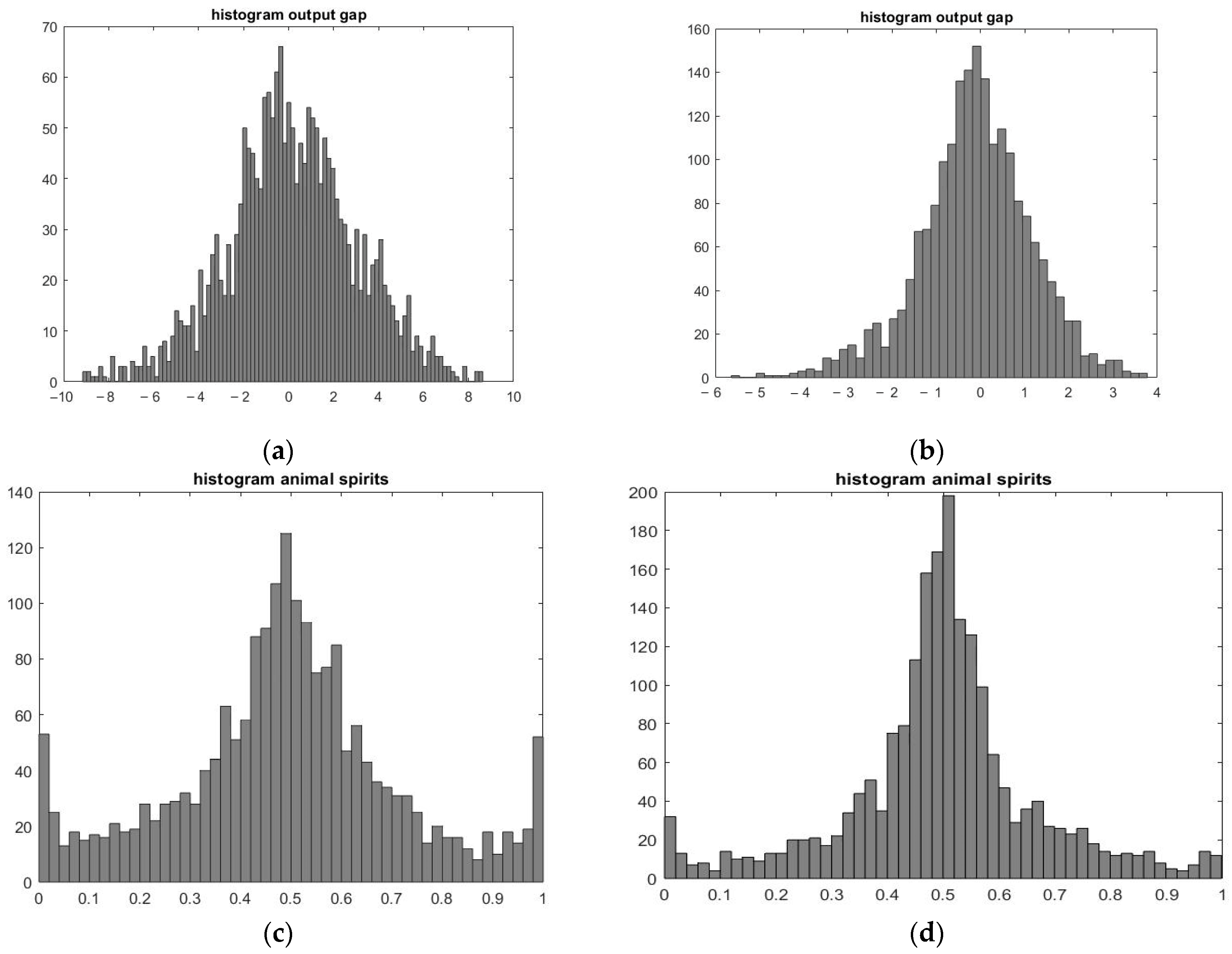In the opposite case, the degree of cheerfulness is equal to the share of fundamentalist agents ${\alpha }_{f,t}$ (Equations (33) and (34)). In this case, the constructed histogram of vital forces is closely related to the histogram of the frequency distribution of the output gap (Figure 1) (In the future, due to the limited format, histograms of the output gap and inflation will not be presented).

Therefore, when the curve in the vitality histogram reaches a value of 1, all agents predict a positive output gap and are optimistic; when the curve reaches a value of 0, no agent predicts a positive output gap, and they become pessimistic. In fact, in this case, they all expect a negative output gap. Thus, the histogram of the frequency distribution of the vitality concentration variable reflects the level of optimism and pessimism of agents regarding the forecast of the production gap.

Figure 1 shows histograms of the frequency distribution of a given output gap (a and b) and the animal variable spirit (c and d) for the two models being compared. A histogram of the standard (In the future, all models other than the closed economy model will be called semi-open economy models) semi-open economy model under study is presented on the left side with the coefficients from Table 1. On the right side (b and d), there is a histogram of the closed economy model (coefficients ${\omega }_2=0,26$${\omega }_3=0,\alpha =0)$. The frequency distribution of the output gap shows extreme deviations from the normal distribution with very thick tails, which suggests booms and busts with a large amplitude. It happens due to the increasing strength of the vital forces of the agents, which is confirmed by the corresponding histogram of the vital forces (below). Comparing the histograms of the vital forces of the standard model (a and c) and the closed economy model (b and d), we can see that there is more pronounced concentration of vital forces in the extreme values of 0 and 1 in the standard model, as well as in the middle of the distribution. This feature is a key explanation for deviations in the dynamics of the evolution of variables from normal indicators. The closed economy model is characterized by a lower degree of concentration of vital forces at extreme values and in the middle of the distribution. However, the distribution of the concentration of vital forces in this model, like in the first one, has “fat tails” that characterize abnormality. Since the degree of optimism and pessimism of agents in the first model is much higher than in the second one, the standard model of a semi-open economy is subject to stronger cyclical movement with greater amplitude compared to the model of a closed economy.

From Table 1 and Equation (9), it follows that the degree of price rigidity depends on the parameter ${\kappa }_p$. The value of this parameter corresponding to the values of the coefficients in Table 1 is equal to 0.086. As the value of this parameter increases, the degree of price rigidity decreases, and accordingly, their flexibility increases. Therefore, as an example, Figure 2 shows a histogram of the frequency distribution of the degree of optimism and pessimism for the studied model of a semi-open economy with values ${\kappa }_p$ = 0.2 (left) and ${\kappa }_p$ = 0.5 (right), that is, for models with a more flexible price compared to the models shown in Figure 1.

The given histogram is characterized by a higher degree of optimism and pessimism of agents and thicker tails at more rigid prices (${\kappa }_p$ = 0.2) compared to the histogram at more flexible prices (${\kappa }_p$ = 0.5). The concentration of the vital forces of agents in the middle of the distribution in the second histogram has decreased, and the above model with more flexible prices is already characterized by the normality of the dynamics of the variables. As before, the first model (${\kappa }_p$ = 0.2) is more susceptible to cyclic movement with a larger amplitude compared to the second one (${\kappa }_p$ = 0.5).

Thus, extreme values of vitality (abnormal spirit) explain the thick tails observed in the output gap distribution. The interpretation of this result is as follows. The model under study demonstrates self-sustaining oscillations between optimism and pessimism (emotional states). When the number of agents with optimistic forecasts exceeds the number of agents with pessimistic forecasts, this leads to a widening of the production gap. The latter, in turn, justifies those who made optimistic forecasts. This then attracts more agents to become optimists. When a market is subject to cyclical fluctuations in optimism (or pessimism), this can lead to a situation in which almost all market participants become optimists (pessimists), which in turn can provoke a strong increase (decrease) in economic activity.

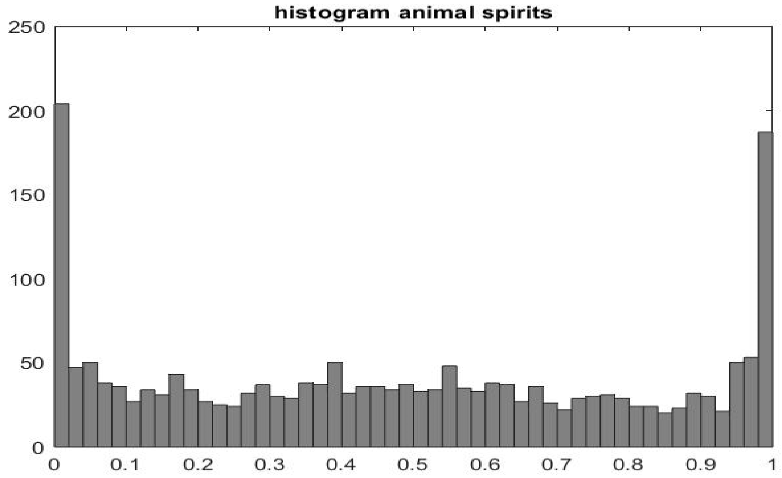
Figure 3 shows a histogram of the frequency distribution of the degree of optimism and pessimism for a model with an increased share of the import component as a factor of production ($\alpha =0.6)$, which is characterized by even greater cyclicality compared to previous histograms due to an increased and almost equal share of optimists and pessimists.

Thus, it is possible to conclude that a more open economy (in our case, semi-open) is more likely to be subject to cyclical movements with greater amplitude compared to a closed economy and abnormal changes in variables.

Figure 4 shows a strong cyclical movement of the output gap and price inflation in the behavioral model under study, as well as the degree of optimism and pessimism of agents, which corresponds to Figure 1a,c.

The source of these cyclical movements is the weight of optimists and pessimists in the market. As DeGrauwe notes [22], “in fact, the model generates endogenous waves of optimism and pessimism. In some periods, pessimists prevail, which leads to below-average output growth. These pessimistic periods are followed by optimistic ones, when optimistic forecasts prevail, and output growth rates are above average”. These waves of optimism and pessimism are inherently unpredictable.

The studied cycles in production, which occur within the system, became possible due to a mechanism that can be described as follows: A sequence of random external shocks creates conditions under which one of two forecasting rules, for example, optimistic, in which agents expect positive changes in production, ensures higher forecast accuracy, that is, lower forecast errors. This attracts agents who previously held a pessimistic rule, according to which they expected negative changes in production. This effect encourages optimistic assumptions in forecasts, for example, regarding the production gap, and this stimulates aggregate demand. As a result, optimistic sentiments become self-fulfilling, leading to an economic boom. However, at some point, negative random effects begin to undermine confidence in optimistic forecasts. Pessimistic sentiments become attractive again, and this leads to an economic downturn.

It can be shown that periods of economic boom and bust coincide with the shares of extrapolators and fundamentalists in the market. In Figure 4, under the graph of the cyclical movement of the output gap, there is a graph characterizing the change in the degree of cheerfulness (b) on the market. From this graph, it can be seen that the positive peaks on the output gap dynamics graph correspond to the values on the animal spirit change graph, close to one, and negative values of the output gap correspond to animal spirit values close to zero spirits. When the index is 0.5, most agents follow the fundamentalist rule; that is, they expect the output gap to return to zero (its steady-state value). The frequency representation of this graph corresponds to the vitality histogram of Figure 1a,c. The correlation coefficient between the output gap and animal spirit graphs is equal to 0.878.

In rational expectations macroeconomic models, only exogenous shocks are relevant in explaining changes in output and inflation. The behavioral model contains important endogenously generated dynamics that explain changes in output and inflation and influence the transmission of these exogenous shocks. The realization of shocks occurred after a period equal to 100 units. It should be noted that the behavioral model differs from the standard New Keynesian model in that, in the former, the timing of the shock is important. The same shocks applied at different times can have very different short-run effects on inflation and output due to different agent sentiments. This is not the case in the standard New Keynesian model with rational expectations: the same shock always has the same effect regardless of the time of its occurrence.

The behavioral model is non-linear. Therefore, in the pre- and post-shock periods, it is necessary to take into account random disturbances, which are the same for the series with and without shock. The simulations were repeated 1000 times with 1000 different implementations of random perturbations. The average impulse response was then calculated along with the standard deviation. Shock sizes were equal to one standard deviation.

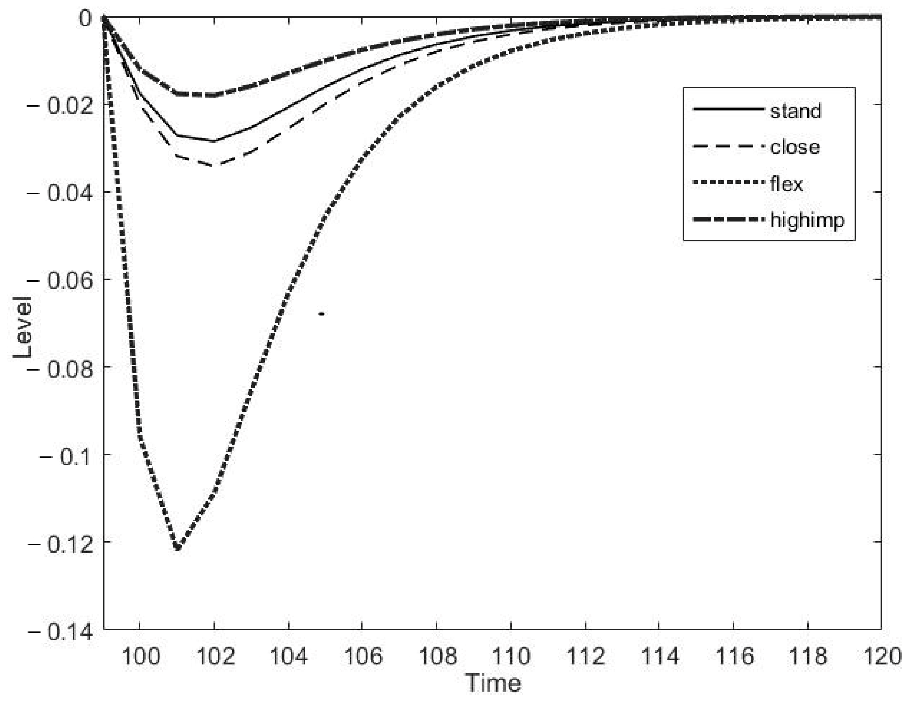
The analysis of interest rate shocks on inflation and the output gap is of particular importance for the implementation of effective monetary policy by the federal authorities. Figure 5 shows the impact of a positive interest rate shock on inflation in the behavioral model of a standard semi-open economy (stand), a closed economy (close), a model with flexible prices (flex), and an increased share of the import component in production (highimport).

From the analysis of impulse responses, it follows that inflation reacts most strongly (decrease) to a positive interest rate shock in a model with prices that are more flexible compared to other prices, which is obvious. An interest rate shock in a closed economy model has the least impact on inflation. As the import component of output increases, the interest rate shock increases the reduction in inflation by reducing production costs. This decrease is not entirely understandable since, as interest rates rise, imported components used in production become more expensive. Probably, the unbounded rationality of agents allows them to “look for workarounds” and purchase imported components at lower prices.

Figure 6 shows the effect of a positive interest rate shock on the output gap of the behavioral model of a standard semi-open economy (stand), a closed economy (close), a model with flexible prices (flex), and a high share of imports in production (highimport).

The output gap responds (decreases) most strongly to a positive interest rate shock in the model with an increased share of imports in output, which is obvious as imports become more expensive. The reduction in the output gap in the closed economy model and, especially, in the model with more flexible prices (compared to the standard semi-open economy model) is weaker. The latter is due to the fact that, as was noted above, in a model with more flexible prices, inflation reacts (declines) more strongly to a positive interest rate shock, and this has the least impact on the economic activity of producers.

It is also of interest to analyze the impact of a technology shock on the model variables. Figure 7 shows the impact of a positive technology shock on inflation of the behavioral model of a standard semi-open economy (stand), a closed economy (close), a model with flexible prices (flex), and an increased share of the import component in production (highimport).

The negative output gap in Figure 7 is due to the fact that, as a result of a technology shock, actual output grows slower than the potential for a given monetary policy. The largest reduction in inflation with a positive technology shock is observed for the model with more flexible prices compared to the standard model, which is obvious. The smallest reduction in inflation during a technology shock is observed for a model with a higher import component in output compared to the standard model, which is associated with increased costs of using imports.

The existence of endogenous movements of optimism and pessimism has important implications for monetary policy. In standard New Keynesian rational expectations models, any attempt to reduce output volatility via the use of interest rate instruments results in increased inflation volatility. In other words, if the monetary authorities decide to increase their desire to stabilize output fluctuations, this will be achieved by increasing inflation volatility.

The influence of the monetary policy of the federal authorities (in this case, the Central Bank) on the behavior of economic agents for various values of the parameters in the Taylor rule was carried out using the analysis of trade-offs between changes in output and inflation in the studied model with bounded rationality of agents. The purpose of this analysis is to study the capabilities of the Central Bank to stabilize business cycles.

In order to show the existence of trade-offs, we will construct a relationship between the volatility of the output gap and the volatility of inflation in the studied model of a semi-open economy for certain values of the parameter ${\phi }_{\pi }$ in the Taylor rule, changing the parameter at the output gap ${\phi }_y$ from 0 to 1 (keeping the parameter ${\phi }_{\pi }$ constant). For each value, ${\phi }_y$ the standard deviations of the output gap and inflation are calculated. The standard deviation of inflation is plotted on the vertical axis, and the standard deviation of the output gap is plotted on the horizontal axis. The results obtained for three values ${\phi }_{\pi }$ = 1.2, 1.5, and 2.0 are presented in Figure 8.

From Figure 8, it follows that the results obtained are non-linear. The top point on curve A with ${\phi }_{\pi }$ = 1.2 corresponds to the situation when the central bank sets ${\phi }_y$ = 0, i.e., does not try to stabilize the output gap at all. This means that for a given value, ${\phi }_{\pi }$ increasing the output ${\phi }_y$ gap stabilization parameter reduces both output volatility (which is obvious) and inflation volatility (not obvious). The explanation is that by stabilizing the output gap, the central bank helps stabilize the waves of optimism and pessimism that are the source of volatility not only in the output gap but also in inflation.

However, this situation has its own limitations. The central bank may exceed its efforts to stabilize output. This is reached where the curves in Figure 8 reach a minimum point and become negatively sloped lines, i.e., too much output gap stabilization undermines the credibility of the inflation target. That is, at some point, the central bank must choose between stabilizing the output gap and stabilizing inflation.

Similar trade-offs between the volatility of inflation and the output gap with an increased share of the imported component as a factor of production $(\alpha =0.6)$ are shown in Figure 9. Unlike the previous case, this figure does not have negatively inclined lines (at the extreme left points of the curved lines); that is, the ability of the Central Bank to stabilize the gap output is sufficient due to lower marginal costs of inflation and “bypassing expensive imports” (Figure 5).

The results shown in Figure 8 and Figure 9 may be useful in carrying out monetary policy to stabilize the variables considered.

5. Discussion

It should be noted first of all that the investigated model of semi-open economy with bounded rationality of agents is original. Therefore, the results obtained in this model can be compared with the results of only a limited number of behavioral models. In addition, only the results obtained for models with the same rules of formation of expectations of economic agents can be compared with each other. Therefore, there is only a limited number of works that fulfill these requirements. These are, first of all, the works of De Grauwe P. [21,22,23].

The behavior of economic agents with boundedly rational expectations in models with the presence of the import component as a factor of production has a number of peculiarities compared to models where this component is absent. This difference is particularly clear in the study of the impulse response functions of inflation and the output gap to technology and interest rate shocks (Figure 5, Figure 6 and Figure 7) and in the analysis of the trade-offs between the volatility of inflation and the output gap due to the Taylor rule of monetary policy (Figure 8 and Figure 9). The presence of these differences in the context of the formation of agents’ expectations is associated with different degrees of concentration of vitality at the extremes and in the middle on the histograms of the frequency distribution of the studied variables and the level of optimism and pessimism (Figure 1, Figure 2 and Figure 3). Waves of optimism and pessimism are the source of volatility not only of the output gap but also of inflation. The difference in the degree of concentration of vital leads to the fact that the model of a semi-open economy is subject to stronger cyclical movement with a larger amplitude compared to the model of a closed economy.

The graphs of cyclical movement of the output gap and price inflation in the studied standard behavioral model of a semi-open economy ($\alpha =0.3$), shown in Figure 4, qualitatively coincide (The amplitudes of cyclical movements of the output gap and inflation in the model under study are proportional to similar amplitudes of the closed economy model [21,22,23]) with similar results obtained by De Grauwe P. [21,22,23] for the behavioral model of the closed economy, i.e., the ratio of the amplitudes of fluctuations of the studied variables for the compared models is approximately the same. This result is expected since, in both cases, cyclical fluctuations are caused by endogenous waves of optimism and pessimism.

The comparative analysis of the impulse response functions is unparalleled in the cited papers [21,22,23]. The detailed discussion of the results presented in the text in Figure 5, Figure 6 and Figure 7 was conducted from the perspective of macroeconomic dynamics. At the same time, the explanation of the increase in the decline in inflation with the growth of the import component of output under an interest rate shock (Figure 5) is difficult to explain. In the context of bounded rationality of agents, this result is easily explainable. As it follows from the analysis of trade-offs between changes in output and inflation (Figure 9), as the share of imports in output increases, the Central Bank’s ability to stabilize the business cycle increases due to the increased degree of optimism and pessimism of agents.

The study of the trade-offs between output and inflation changes in the model under study is important for identifying the ability of the Central Bank to stabilize business cycles. The analysis of the trade-offs in the standard economy model ($\alpha =0.3$) between output and inflation changes in the model under study with bounded rationality of agents shows that at a certain point, the Central Bank has to choose between stabilizing the output gap and inflation. The reason for this result is that, initially, stabilizing the output gap has the effect of reducing the “fat tails” in the histogram of the frequency distribution of the degree of vital forces. In other words, stabilization reduces the degree of optimism and pessimism of agents. As long as they are intense, stabilization (the output gap) reduces the volatility of inflation and output. When these “fat tails” are sufficiently reduced, the standard negative trade-off result appears. As a result, most agents follow the fundamentalist rule (Figure 4), and the central bank’s ability to stabilize the business cycle is reduced. Note that the obtained result for the studied model of the standard economy coincides with a similar result obtained by the author [21].

The effect of negative trade-off is leveled with the increase in the share of imports as a factor of production ($\alpha =0.6$), i.e., the Central Bank’s capacity to stabilize the output gap is sufficient due to the reduction in marginal inflationary costs. This result is different from the similar conclusion obtained in [21] for the closed economy model. The reason is that a more open economy is characterized by an increased degree of optimism and pessimism of agents compared to a less open economy (Figure 1 and Figure 3). For models with rational agents’ expectations [1,2], the curves in Figure 8 and Figure 9 should always have a negative slope. Therefore, the results obtained in the trade-off analysis for the studied model with bounded rationality of agents have an important significance, which is that the rational expectations hypothesis is more consistent with a closed economy than with an open one.

6. Conclusions

In accordance with the purpose of the work, changes, and features of the behavior of economic agents in the new Keynesian behavioral model of a semi-open economy with cognitive limitations of agents were analyzed. The relevance of the study is caused by the peculiarities of the functioning of the economy during the sanctions period. We have studied a model in which the import component is a factor of production, along with labor. At the same time, households, due to sanctions, consume only domestically produced goods and products. At the same time, forecasting the output gap and price inflation occurs using fundamentalist and extrapolation rules. The weight shares of agents applying these heuristics change endogenously, which generates endogenous waves of optimism and pessimism.

From the analysis of the histograms of the frequency distribution of the degree of vitality of the models, we can conclude that a more open economy (in our case, semi-open) is subject to cyclical movements caused by waves of optimism and pessimism, with a deeper amplitude compared to a closed economy.

Analysis of the impulse responses of the interest rate shock and technology shock made it possible to identify the influence of the increased share of the import component as a factor of production and price flexibility on the studied variables.

An analysis of the trade-offs between inflation volatility and the output gap showed their non-linear nature (in contrast to standard models with rational expectations). The explanation is that by stabilizing the output gap, the central bank helps stabilize the waves of optimism and pessimism that are the source of volatility not only in the output gap but also in inflation. However, at a certain point, too much stabilization of the output gap undermines the credibility of the inflation target, the economy becomes more flexible, and the central bank’s ability to stabilize the business cycle is reduced. This situation does not exist with an increase in the import component of product output. The result indicates that the rational expectations hypothesis is more consistent with a closed economy than with an open economy.

The main limitation of the approach used in this paper is that it is currently applicable to low- and medium-dimensional models. Applying it to large-scale structural models that cannot be reduced is computationally difficult.

In addition, there are many factors in the domestic economy where sanctions related to import and export restrictions may not fit into the bounded rationality framework. One such factor is corruption at the domestic level, where even the absence of international ties can affect the inflation rate. For example, the authors of the study [47] found that there is both long-run and short-run causality observed between corruption and inflation rate. The study prescribes the implementation of stricter norms to control corruption to reduce social volatility.

The authors are aware that with different heuristic prediction rules than those used in this study, the results of the study may change. Therefore, the next stage of the work is to test the results obtained in this study under different cognitive constraints of the agents of the behavioral model. In addition, it should be noted that government expenditure in the investigated model is exogenous and changes according to the autoregressive law (AR1). With endogenous government expenditures, there is a possibility of analyzing the impact of fiscal policy on agents’ behavior. This is also an incentive for further work with this model.

Finally, we should also note that the article used calibrated data to verify the theory. Since information from various sources on macroeconomic indicators, including for individual countries and regions, is currently available, the next stage of the authors’ work will be to analyze the empirical validity of the results obtained.