Dual-Graph-Regularization Constrained Nonnegative Matrix Factorization with Label Discrimination for Data Clustering

Abstract

NONNEGATIVE matrix factorization (NMF) is an effective technique for dimensionality reduction of high-dimensional data for tasks such as machine learning and data visualization. However, for practical clustering tasks, traditional NMF ignores the manifold information of both the data space and feature space, as well as the discriminative information of the data. In this paper, we propose a semisupervised NMF called dual-graph-regularization-constrained nonnegative matrix factorization with label discrimination (DCNMFLD). DCNMFLD combines dual graph regularization and prior label information as additional constraints, making full use of the intrinsic geometric and discriminative structures of the data, and can efficiently enhance the discriminative and exclusionary nature of clustering and improve the clustering performance. The evaluation of the clustering experimental results on four benchmark datasets demonstrates the effectiveness of our new algorithm.

1. Introduction

The initial step of many data mining methods involves reducing the dimensionality of the original high-dimensional data to obtain a condensed low-dimensional representation of the data [1,2,3]. This is done to facilitate subsequent tasks, such as learning and visualization. Several commonly employed methods for dimensionality reduction are principal component analysis [4], singular value decomposition [5], linear discriminant analysis [6], concept decomposition [7], and nonnegative matrix factorization (NMF) [8,9]. These methods are all based on matrix factorization approaches. NMF, for instance, aims to decompose a given nonnegative data matrix $X$ into a product of two lower-order nonnegative matrices $U$ and $V$. The objective is for the product of $U$ and $V$ to approximate $X$ under a specific distance metric [8,9]. NMF has been proven to be a powerful technique for reducing the dimensionality of high-dimensional data and is widely employed in feature extraction [10,11], data mining [12,13,14], computer vision [14,15] and various other applications [16,17,18,19,20]. However, the standard NMF has several shortcomings that require further improvement. For instance, Cai et al. [21] highlighted one of these shortcomings: the failure of NMF to consider the geometric structure information within the data space. This information is crucial for tasks such as data clustering and classification [21,22]. To address this issue, Cai et al. [21] proposed a method called graph regularization NMF (GNMF), which incorporated geometric information by constructing a p-nearest neighbor graph. Building upon the concept of GNMF, Shang et al. [23] introduced a novel algorithm known as dual graph regularization NMF (DNMF). DNMF enhanced the preservation of geometric information by constructing two p-nearest-neighbor graphs: one in the data space and another in the feature space.

The standard NMF is considered unsupervised learning as it does not utilize label information from data [8,9]. However, researchers have observed that incorporating a small amount of labeled data with unlabeled data can significantly enhance the performance of learning algorithms in various machine-learning tasks [21,22,23]. Consequently, efforts have been made to integrate label information into NMF frameworks, resulting in the development of several semisupervised NMF algorithms [24,25]. For instance, Lee et al. [26] proposed a semisupervised NMF algorithm that incorporated partial label information constraints into NMF. Similarly, Liu et al. [27] introduced a constrained NMF (CNMF) method that embedded label information into the main objective function of NMF, ensuring that data points with the same class label shared the same representation in the new representation. In the discriminative NMF method [28], partial label information is employed as a discriminant constraint, aligning data points with the same label on the same axis in the new representation. However, neither CNMF nor discriminative NMF integrated the local geometric structure of the data. Thus, graph-regularized semisupervised NMF methods have been proposed, which incorporate local manifold regularization into CNMF and discriminative NMF, thereby preserving local structures and enhancing the discrimination of new representations [29,30].

Based on previous works, such as those for DNMF [23] and CNMF [27], Sun et al. [31] introduced a new method called dual graph regularization constraint NMF (DCNMF). This method incorporated the geometric structure of data manifolds and feature manifolds and labeling information. To further enhance the discriminative ability of new representations, Sun et al. [32] proposed sparse dual graph regularization NMF (SDGNMF), which included sparse constraints in DCNMF. Li et al. [33] introduced orthogonality constraints based on coefficient matrices, resulting in a semisupervised dual graph regularization NMF (SDGNMF_BO). In semisupervised NMF methods, researchers typically evaluate the effectiveness of a new representation $V$ using the K-means method in clustering experiments. However, Xing et al. [34,35] noticed that the new representation obtained from these methods may not be suitable for the K-means method because of the impact of random initialization, which can result in the misclassification of labeled data points. To address this limitation, Xing et al. [34] proposed graph-regularized NMF with labeled discrimination (GNMFLD), which employed an alternative clustering method to predict the labels of unlabeled data points in clustering experiments.

From the above analysis, we found that the DCNMF algorithm, as discussed by Xing et al. [34], has certain shortcomings. Meanwhile, the GNMFLD algorithm does not effectively utilize manifold information within the feature space. In this paper, we propose a novel approach called dual-graph-regularized constrained NMF with label discrimination (DCNMFLD) to overcome the above shortcomings by fully exploiting the advantages of DCNMF and GNMFLD.

This paper is structured as follows: Section 2 provides a review of standard NMF and several related semisupervised NMF algorithms. Section 3 presents the objective function, optimization scheme, and theoretical analysis of DCNMFLD. Section 4 presents a series of clustering experiments conducted to demonstrate the efficacy of our proposed method. Finally, Section 5 concludes the paper.

2. Related Works

2.1. NMF

Consider a nonnegative data matrix $X=[x_1,\dots ,x_n]\in R^{m\times n}$, where $n$ is the number of data points and $m$ is the dimension of the data points. Each column $x_i\in R^m$ is a data point with $m$-dimensional features. Given a reduced dimension $r$, the goal of standard NMF [8] is to decompose $X$ into two low-rank nonnegative matrices, a base matrix $U\in R^{m\times r}$ and a coefficient matrix $V\in R^{n\times r}$, so that the matrix $X$ is approximated by a product of matrix $U$ and matrix $V$. Using the Frobenius norm to measure the approximation, the problem of standard NMF can be stated as:

$$\begin{array}{r}\underset{U,V}{\min }{O}_{NMF}={‖X-U{V}^T‖}_F^2, \\ s.t. U\ge 0,V\ge 0,\end{array}$$

(1)

Obtaining the global minimum for $O_{NMF}$ is hard because the objective function $O_{NMF}$ is not convex in both $U$ and $V$ together. Previously [9], the multiplicative iterative updating algorithm presented by Lee and Seung was used to find the local minimum of $O_{NMF}$ as follows: $U=U\frac{XV}{U{V}^{T}V},V=V\frac{X^{T}U}{V{U}^{T}U}.$

2.2. CNMF

Standard NMF belongs to unsupervised dimensionality reduction methods, which cannot utilize the label information of data points. Liu et al. [27] proposed a semisupervised NMF, called CNMF, which takes the label information as additional hard constraints so that the data points from the same class should be merged in the new representation space. We considered the data points as belonging to $c$ classes, where $l$ data points are labeled and the rest $n-l$ data points are unlabeled. Using the available label information, we define the indicator matrix $C\in R^{l\times c}$ as:

$$C_{ij}=\left\{\begin{array}{l}1, x_i \mathrm{belongs} \mathrm{to} \mathrm{the} j\mathrm{th} \mathrm{cluster},\\ 0, \mathrm{otherwise}.\end{array}\right.$$

(2)

Based on the indicator matrix $C$, a label constraint matrix $A\in R^{n\times (c+n-l)}$ is constructed as follows:

$$A=\left(\begin{array}{cc}{C}_{l\times c}& 0\\ 0& I_{n-l}\end{array}\right),$$

(3)

where $I_{n-l}$ is an $(n-l)\times (n-l)$ identity matrix and $0$s are zero matrices with compatible dimensions. With the help of an auxiliary matrix $Z\in R^{(c+n-l)\times r}$, the data matrix $X$ is approximated as $X\approx U{V}^T\approx U{(AZ)}^T$. The CNMF problem has the following form:

$$\begin{array}{l}\underset{U,Z}{\min }{O}_{CNMF}={‖X-U{Z}^T{A}^T‖}_F^2,\\ s.t. U\ge 0,Z\ge 0.\end{array}$$

(4)

2.3. GNMF

The standard NMF has some limitations. For instance, for any given local optimal solution $(U,V)$ of NMF: $X\approx U{V}^T$, we can find that any given $\lambda >0$, $(\lambda U,\frac{1}{\lambda }V)$ is also the local optimal solution with the same residue ${‖X-U{V}^T‖}_F^2$. In addition, the initial values of $(U,V)$ in the update rules are randomly generated. Therefore, the $(U,V)$ we obtained in (1) may not be suitable for our subsequent work. To address this, we can provide additional information to guide NMF in generating custom new representations. As we know, data space’s geometric structure (e.g., the nearest neighbor relationship) is crucial for clustering performance. We hope the new representations of data points also maintain corresponding geometric structure in low dimensional space. To achieve this goal, Cai et al. proposed the GNMF method [21,22] by incorporating a regularizer into NMF based on the graph Laplacian of data space. Suppose the data points are represented by $V=[v_1^T,v_2^T,\dots ,v_n^T]\in R^{n\times r}$ in a new representation space. Then, the Laplacian graph of the data space is defined as

$$\begin{array}{ll}{R}_1& =\frac{1}{2}{\displaystyle \sum _{i,j}^n{‖v_i-v_j‖}_F^2{W}^V}=({\displaystyle \sum _{i=1}^n{v}_i{v}_i^T{D}_{ii}^V}-{\displaystyle \sum _{i,j=1}^n{v}_i{v}_j^T{W}_{ij}^V}),\\ & =Tr(V^T{D}^{V}V)-Tr(V^T{W}^{V}V)=Tr(V^T{L}_{V}V),\end{array}$$

(5)

where $Tr(\cdot )$ denotes the trace of a matrix, $W^V$ represents the similarity matrix, $L_V=D^V-W^V$ is the Laplacian matrix, and $D^V$ is a diagonal matrix with elements $d_{ii}{}^V={\displaystyle {\sum }_j{w}_{ij}^v}$. The weight matrix $W^V$ can be constructed using many rules, such as 0–1 weighting, heat kernel weighting, and dot-product weighting. The most used weighting is 0–1 weighting. Then, the element $W_{ij}^V$ can be defined as:

$$W_{ij}^V=\left\{\begin{array}{l}1, if x_j\in N_p(x_i),\\ 0, otherwise,\end{array}\right.i,j=1,2,\dots ,n,$$

(6)

where $x_j\in N_p(x_i)$ indicates that data point $x_i$ is a p-nearest neighbor of data point $x_j$. By minimizing formula $R_1$, two data points similar in the original data space will also be close in the new representation space. Thus, the term $R_1$ can preserve the geometric structure of the data space. With the term $R_1$, the problem of GNMF is stated as:

$$\begin{array}{l}\underset{U,V}{\min }{O}_{GNMF}={‖X-U{V}^T‖}_F^2+\alpha \mathrm{Tr}\left(V^T{L}_{V}V\right),\\ s.t. U\ge 0,V\ge 0,\end{array}$$

(7)

where $\alpha >0$ is a regularized parameter.

2.4. DNMF

Researchers have found that not only does the data space have an intrinsic geometric structure, but also feature space. Thus, the graph Laplacian of the feature space is constructed. Shang et al. [23] proposed DNMF, which utilized graph Laplacians of data space and feature space. Following the way of GNMF, for data $[x_1^T,x_2^T,\dots ,x_m^T]$ and base matrix $U=[u_1^T,u_2^T,\dots ,u_m^T]$, the graph Laplacian of the feature space is formulated as follows:

$$\begin{array}{ll}{R}_2& =\frac{1}{2}{\displaystyle \sum _{i,j}^m{‖u_i-u_j‖}^2{W}^U}=({\displaystyle \sum _{i=1}^m{u}_i{u}_i^T{D}_{ii}^U}-{\displaystyle \sum _{i,j=1}^m{u}_i{u}_j^T{W}_{ij}^U}),\\ & =Tr(U^T{D}^{U}U)-Tr(U^T{W}^{U}U)=Tr(U^T{L}_{U}U),\end{array}$$

(8)

where $L_U=D^U-W^U$ is a Laplacian matrix, $W^U$ is also the weight matrix but in the feature space, and $D^U$ is a diagonal matrix with elements $d_{ii}{}^u={\displaystyle {\sum }_j{w}_{ij}^u}$.

With 0–1 weighting, the elements of $W^U$ can be defined as follows:

$$W_{ij}^U=\left\{\begin{array}{l}1, if x_j^T\in N_p(x_i^T),\\ 0, otherwise,\end{array}\right.i,j=1,2,\dots ,m.$$

(9)

By incorporating the terms $R_1$ and $R_2$ into the NMF, the problem of DNMF is formulated as follows:

$$\begin{array}{l}\underset{U,V}{\min }{O}_{DNMF}={‖X-U{V}^T‖}_F^2+\alpha Tr(V^T{L}_{V}V)+\beta Tr(U^T{L}_{U}U) ,\\ s.t. \mathrm{U}\ge 0,\mathrm{V}\ge 0,\end{array}$$

(10)

where $\alpha$ and $\beta$ are regularized parameters.

2.5. DCNMF

Building upon the concepts of CNMF [27] and DNMF [23], Sun et al. [31] introduced DCNMF, a novel approach that incorporated the geometric structures of both the data space and feature space, as well as the label information of a subset of data points. The problem of DCNMF can be formulated as follows:

$$\begin{array}{l}\underset{U,Z}{\min }{O}_{DCNMF}={‖X-U{Z}^T{A}^T‖}_F^2+\alpha Tr(Z^T{A}^T{L}_{V}AZ)+\beta Tr(U^T{L}_{U}U) ,\\ s.t. \mathrm{U}\ge 0,\mathrm{Z}\ge 0,\end{array}$$

(11)

where $\alpha$ and $\beta$ are also regularized parameters.

2.6. GNMFLD

Xing et al. [34] proposed a semisupervised NMF method called GNMFLD. With the indicator matrix $C$, which is defined in (2), a partly cluster indicator matrix $Y$ is constructed as

$$Y=\left(\begin{array}{c}C\\ 0_{(n-l)\times c}\end{array}\right).$$

(12)

In addition, a projection operator $P_{\mathrm{\Omega }}$ is defined as

$$P_{\mathrm{\Omega }}{(V)}_{ij}=\left(\begin{array}{l}{V}_{ij}, (i,j)\in \mathrm{\Omega },\\ 0, otherwise,\end{array}\right.$$

(13)

where $\mathrm{\Omega }=\{(i,j)\left|1\le i\le l,1\le j\le c\right.\}$.

With the partly cluster indicator matrix $Y$ in (12) and projection operator $P_{\mathrm{\Omega }}$ in (13), a discrimination term ${‖P_{\mathrm{\Omega }}(V)-P_{\mathrm{\Omega }}(Y)‖}_F^2$ is introduced to NMF, and the problem of GNMFLD can be formulated as

$$\begin{array}{l}\underset{U,V}{\min }{O}_{GNMFLD}={‖X-U{V}^T‖}_F^2+\alpha {‖P_{\mathrm{\Omega }}(V)-P_{\mathrm{\Omega }}(Y)‖}_F^2+\beta \mathrm{Tr}\left(V^{T}LV\right), \\ s.t. U\ge 0,V\ge 0.\end{array}$$

(14)

where $\alpha$ and $\beta$ are regularized parameters.

3. Proposed DCNMFLD

In this section, we introduce the details of DCNMFLD. We construct the objective function of DCNMFLD and provide an iterative update rule scheme to solve it. The convergence of the proposed algorithm is proved, and the computational complexity analysis of the algorithm is given.

3.1. DCNMFLD

DCNMF, an extension of CNMF, incorporates dual graphs (data and feature graph) as constraints to enhance the ability of subspace learning. These dual graphs leverage the inherent geometric structure of the data space and feature space. In clustering tasks, these graphs guide similar new representations to aggregate in the low-dimensional space. However, Xing et al. [34] noted that the clustering accuracy can be affected by the random initialization of the K-means algorithm when the new data representation obtained by CNMF is used. Xing et al. [34] proposed the GNMFLD algorithm to address this issue and used another class label determination mechanism: determine sample $x_i$ to class $k$, if $k=\arg \underset{s}{\max } v_{js}$. To match this class label determination mechanism, they proposed a discriminative term ${‖P_{\mathrm{\Omega }}(V)-P_{\mathrm{\Omega }}(Y)‖}_F^2$ in GNMFLD. For $V=\left(\begin{array}{l}{V}_1\\ V_2\end{array}\right)$ with $V_1\in R^{l\times c}$, then by term ${‖P_{\mathrm{\Omega }}(V)-P_{\mathrm{\Omega }}(Y)‖}_F^2$, it gives the approximation $V_1\approx C$. Thus, the new representation of labeled data should approximate a One-Hot vector (only one element being 1 and the rest being 0). Guided by the regularization graph, all data sharing the same label should converge towards this One-Hot vector. Therefore, based on the class label determination mechanism they adopted, the position of element 1 signifies the category to which the new representation belongs, thereby eliminating the uncertainty associated with using K-means. Thus, the discriminative term ${‖P_{\mathrm{\Omega }}(V)-P_{\mathrm{\Omega }}(Y)‖}_F^2$ achieves a “One-Hot scaling” effect. In view of this, to obtain more discriminative new representations and avoid using K-means in clustering tasks, we incorporated term ${‖P_{\mathrm{\Omega }}(V)-P_{\mathrm{\Omega }}(Y)‖}_F^2$ of GNMFLD into DCNMF and proposed the DCNMFLD algorithm. Based on the above details in (11) and (14), the problem of DCNMFLD is stated as follows:

$$\begin{array}{l}\underset{U,Z}{\min }{O}_{DCNMFLD}={‖X-U{Z}^T{A}^T‖}_F^2+\alpha Tr(Z^T{A}^T{L}_{Z}AZ)+\beta Tr(U^T{L}_{U}U)+\gamma {‖P_{\mathrm{\Omega }}(AZ)-P_{\mathrm{\Omega }}(Y)‖}_F^2,\\ s.t. \mathrm{U}\ge 0 , \mathrm{Z}\ge 0.\end{array}$$

(15)

To simplify the form of the term ${‖P_{\mathrm{\Omega }}(AZ)-P_{\mathrm{\Omega }}(Y)‖}_F^2$, we introduce an auxiliary matrix $B\in R^{n\times (c+n-l)}$ as:

$$B=\left[\begin{array}{cc}{C}_{l\times c}& 0\\ 0& 0_{(N-l)\times (N-l)}\end{array}\right],$$

(16)

where $C_{l\times c}$ is also defined in (2) and $0_{n-l}$ is an $(n-l)\times (n-l)$ zeros matrix.

We find that ${‖P_{\mathrm{\Omega }}(AZ)-Y‖}_F^2={‖BZ-Y‖}_F^2$. Then, the formulations of DCNMFLD can transformed into

$$\begin{array}{l}\underset{U,Z}{\min }{O}_{DCNMFLD}={‖X-U{Z}^T{A}^T‖}_F^2+\alpha Tr(Z^T{A}^T{L}_{Z}AZ)+\beta Tr(U^T{L}_{U}U)+\gamma {‖BZ-Y‖}_F^2,\\ s.t. \mathrm{U}\ge 0 ,\mathrm{Z}\ge 0.\end{array}$$

(17)

If we call the discriminative mechanism in DCNMF as “label hard constraint”, and in GNMFLD, a “One-Hot scaling”,

Table 1. The comparison between our method and related methods.

Methods	Label Hard Constraint	One-Hot Scaling	Data Graph	Feature Graph
GNMFLD	×	√	√	×
DCNMF	√	×	√	√
DCNMFLD	√	√	√	√

gives an intuitive comparison of DCNMF, GNMFLD and our DCNMFLD. Obviously, our method combines more constraints to obtain our custom representation.

3.2. Optimization

The objective function $O_{DCNMFLD}$ in (17) is nonconvex in both variables $U$ and $Z$. Therefore, obtaining the global minimum solution is unrealistic. In the following, we use a multiplication iterative updating algorithm [9] to optimize the objective function $O_{DCNMFLD}$. With the properties of the matrix, the objective function $O_{DCNMFLD}$ in (17) can be rewritten as:

$$\begin{array}{l}{O}_{DCNMFLD}=Tr[(X-U{Z}^T{A}^T)T(X-U{Z}^T{A}^T)]+\alpha TrTr(Z^T{A}^T{L}_{Z}AZ)+\beta Tr(U^T{L}_{U}U)\\ +\gamma {\mathrm{Tr}\left(\right(\mathrm{BZ}-\mathrm{Y})}^T(\mathrm{BZ}-\mathrm{Y}))\\ =Tr(X^{T}X-2AZ{U}^{T}X+AZ{U}^{T}U{Z}^T{A}^T)+\alpha TrTr(Z^T{A}^T{L}_{Z}AZ)\\ +\beta Tr(U^T{L}_{U}U)+\gamma Tr([{\left(\mathrm{BZ}\right)}^T\left(\mathrm{BZ}\right)-2{\left(\mathrm{BZ}\right)}^{T}Y+Y^{T}Y\left]\right).\end{array}$$

(18)

Let $\mathrm{\Phi }=\left({\varphi }_{ij}\right)\in R^{M\times K}$ and $\mathrm{\Psi }=\left({\psi }_{ij}\right)\in R^{N\times K}$ be the Lagrange multiplier for the constraints $U\ge 0$ and $Z\ge 0$, respectively. The Lagrange function $L$ can be formulated as follows:

$$L=O_{DCNMFLD}+Tr(\mathrm{\Phi }{U}^T)+Tr(\mathrm{\Psi }{\mathrm{Z}}^T).$$

(19)

Taking the derivatives of $L$ with respect to $U$ and $Z$, we obtain:

$$\begin{array}{l}\frac{\partial L}{\partial U}=-2XAZ+2U{Z}^T{A}^{T}AZ+\beta L_{U}U+\varphi ,\\ \frac{\partial L}{\partial Z}=-2A^T{X}^{T}U+2A^{T}AZ{U}^{T}U-2\gamma B^{T}Y+2\gamma B^{T}BZ+\alpha A^T{L}_{Z}AZ+\mathrm{\Psi }.\end{array}$$

(20)

Using the KKT conditions ${\varphi }_{ij}{u}_{ij}=0$ and ${\psi }_{ij}{v}_{ij}=0$, we obtain:

$$\begin{array}{l}(-2XAZ+2U{Z}^T{A}^{T}AZ+\beta L_{U}U{)}_{ij}{u}_{ij}=0,\\ {(-2A^T{X}^{T}U+2A^{T}AZ{U}^{T}U-2\gamma B^{T}Y+2\gamma B^{T}BZ+\alpha A^T{L}_{Z}AZ)}_{ij}{z}_{ij}=0.\end{array}$$

(21)

Because $L_Z=D^Z-W^Z$ and $L_U=D^U-W^U$, we can arrive at the following updating formula:

$$u_{ij}\leftarrow u_{ij}\frac{{(XAZ+\gamma W_{U}U)}_{ij}}{{\left(U{Z}^T{A}^{T}AZ+\gamma D_{U}U\right)}_{ij}},$$

(22)

$$z_{ij}\leftarrow z_{ij}\frac{{\left(A^T{X}^{T}U+\beta B^{T}Y+\alpha A^T{W}_{Z}AZ\right)}_{ij}}{{\left(A^{T}AZ{U}^{T}U+\beta B^{T}BZ+\alpha A^T{D}_{Z}AZ\right)}_{ij}}.$$

(23)

The optimization of DCNMFLD is summarized in Algorithm 1.

Algorithm 1 DCNMFLD.

Input: matrix $X\in R^{m\times n}$. The regularization parameters $\alpha$, $\beta$ and $\gamma$. The number of neighbors $p$. The clustering number $r$. The maximum iteration number $I$.

Output: matrices $U$ and $Z$. 1:  Initialize $U=rand(m,k)$, $Z=rand(c+n-l,k)$; 2:  Construct the weight matrix $W_Z$ and $W_U$ using (6) and (9), and calculate the matrices $D_Z$ and $D_U$, respectively; 3:  Construct the label constraint matrix $A$ using (3), partly cluster indicator matrix $Y$ using (12), and auxiliary matrix $B$ using (16); 4:  for $t=1,2,\cdots I$ do 5:        Update $U$ by using (22); 6:        Update $Z$ by using (23); 7:  endfor

We present the following theorem for the iterative updating rules (22) and (23):

Theorem 1. 

For $U,Z\ge 0$, the objective function $O_F$ in (17) is nonincreasing under the updating rules in (22) and (23) (i.e., convergent). The objective function is invariant under these updates if and only if U and Z are at a stationary point.

3.3. Convergence Analysis

In this section, we adopt the auxiliary function approach to prove Theorem 1. Notice that the regularized terms in the objective function $O_F$ in (17) are only related to $V$ each other; thus, the updating rules for $U$ (23) are the same as those in (2) in the standard NMF. According to a previous study [8], Theorem 1 is true for $U$ in (23). Thus, we only need to prove that Theorem 1 is true for $V$ in the update rule (22).

Definition 1 

([21]). $G\left(z,z\prime \right)$ is an auxiliary function for $F(z)$ if the following conditions are satisfied: $G\left(z,z\prime \right)⩾F(z)$, $G(z,z)=F(z)$.

Lemma 1. 

If $G\left(z,z\prime \right)$ is an auxiliary function of $F(z)$, then $F(z)$ is nonincreasing under the update:

$$z^{t+1}=\arg \underset{z}{\min }G\left(z,z^t\right).$$

(24)

Proof. 

By Definition 1 and Lemma 1, the following inequality for

$$F\left(z^{t+1}\right)\le G\left(z^{t+1},z^t\right)$$

(25)

can be obtained:

$$F\left(z^{t+1}\right)\le G\left(z^{t+1},z^t\right)\le G\left(z^t,z^t\right)\le F\left(z^t\right).$$

(26)

The equality $F\left(z^{t+1}\right)=F\left(z^t\right)$ holds only if $z^t$ is a local minimum of $F\left(z\right)$. By applying updating rule (23), $z^t$, converges to the local minimum of $F\left(z\right)$.

Now, we will prove that the iterative updating rule (23) for $Z$ is consistent with (24). Let $F_{z_{ab}}(z_{ab})$ denote the part of the objective function relevant to any element $z_{ab}$ in $Z$. Then, the expression of $F_{z_{ab}}(z_{ab})$ is:

$$\begin{array}{ll}{F}_{z_{ab}}(z_{ab})=& {(-2Tr(AZ{U}^{T}X)+Tr(AZ{U}^{T}U{Z}^T{A}^T)}_{ab}+\alpha Tr{(Z^T{A}^T{L}_{Z}AZ)}_{ab}\\ & +\gamma Tr{(Z^T{B}^{T}BZ-2Z^T{B}^{T}Y)}_{ab}.\end{array}$$

(27)

The first-order and second-order derivatives of $F_{z_{ab}}(z_{ab})$ about the variable $z_{ab}$ are

$$F_{z_{ab}}^{\prime }(z_{ab})={(-2A^T{X}^{T}U+2A^{T}AZ{U}^{T}U-2\gamma B^{T}Y+2\gamma B^{T}BZ+\alpha A^T{L}_{Z}AZ)}_{ab},$$

(28)

and

$$F_{z_{ab}}^{″}(z_{ab})=2{(A^{T}A{U}^{T}U)}_{bb}+2\alpha A^T{L}_{aa}A+2\gamma {(B^{T}B)}_{bb}.$$

(29)

□

Lemma 2. 

The function

$$\begin{array}{ll}G\left(z_{ab},z_{ab}^t\right)=& F_{z_{ab}}\left(z_{ab}^t\right)+F{\prime }_{z_{ab}}\left(z_{ab}^t\right)\left(z_{ab}-z_{ab}^t\right)\\ & +\frac{{\left(A^{T}AZ{U}^{T}U+\gamma B^{T}BZ+\alpha A^T{D}_{Z}AZ\right)}_{ab}}{z_{ab}^t}{\left(z_{ab}-z_{ab}^t\right)}^2,\\ \end{array}$$

(30)

is an auxiliary function for $F_{z_{ab}}(z_{ab})$.

Proof. 

Apparently, $G\left(z,z\right)=F_{z_{ab}}\left(z\right)$. To show $G\left(z_{ab},z_{ab}^t\right)⩾F_{z_{ab}}\left(z_{ab}\right)$, we compare the auxiliary function to the Taylor series expansion:

$$F_{z_{ab}}\left(z_{ab}\right)=F_{z_{ab}}\left(z_{ab}^t\right)+F_{z_{ab}}^{\prime }\left(z_{ab}^t\right)\left(z_{ab}-z_{ab}^t\right)+\frac{1}{2}{F}_{z_{ab}}^{\prime \prime }\left(z_{ab}^t\right){\left(z_{ab}-z_{ab}^t\right)}^2.$$

(31)

We can have that $G\left(z_{ab},z_{ab}^t\right)\le F_{z_{ab}}\left(z_{ab}\right)$ is equivalent to check the inequality:

$$\frac{{\left(A^{T}AZ{U}^{T}U+\gamma B^{T}BZ+\alpha A^T{D}_{Z}AZ\right)}_{ab}}{z_{ab}^t}\ge {(A^{T}A{U}^{T}U)}_{bb}+\alpha A^T{L}_{aa}A+\gamma {(B^{T}B)}_{bb}.$$

(32)

Because

$$(A^{T}AZ{U}^{T}U)={\displaystyle \sum _l(A^{T}AZ)(U^{T}U)}\ge (A^{T}AZ)(U^{T}U)\ge {\displaystyle \sum _l(A^{T}A)z^t(U^{T}U)}\ge z^t(A^{T}A)(U^{T}U),$$

(33)

$$\alpha A^T{D}^{Z}AZ=\alpha {\displaystyle \sum _l{A}^T{D}^{Z}A{z}^t}\ge \alpha A^T{D}^{Z}A{z}^t\ge \alpha A^T(D^Z-W^Z)A{z}^t\ge \alpha A^T{L}^{Z}A{z}^t,$$

(34)

and

$$\gamma {(B^{T}BZ)}_{ab}=\gamma {\displaystyle \sum _l(B^{T}B)z^t}\ge \gamma {(B^{T}B)}_{bb}{z}_{ab}^{(t)}.$$

(35)

Therefore, the inequality $G\left(z_{ab},z_{ab}^t\right)\le F_{z_{ab}}\left(z_{ab}\right)$ is founded and Lemma 2 is proven.

Now, we prove Theorem 1. Replacing $G\left(z,z\prime \right)$ in (30) by (33), the minimum is obtained by solving:

$$\begin{array}{l}\frac{\partial G\left(z_{ab},z_{ab}^t\right)}{\partial z_{ab}}=F{\prime }_{z_{ab}}\left(z_{ab}^t\right)+\frac{2{\left(A^{T}AZ{U}^{T}U+\gamma B^{T}BZ+\alpha A^T{D}_{Z}AZ\right)}_{ab}}{z_{ab}^t}\left(z_{ab}-z_{ab}^t\right)=0,\\ \end{array}$$

which can yield:

$$z_{ij}\leftarrow z_{ij}\frac{{\left(A^T{X}^{T}U+\gamma B^{T}Y+\alpha A^T{W}_{Z}AZ\right)}_{ij}}{{\left(A^{T}AZ{U}^{T}U+\gamma B^{T}BZ+\alpha A^T{D}_{Z}AZ\right)}_{ij}}.$$

(36)

Obviously, (36) is the same with (23). By Lemma 2, the objective function in (8) is nonincreasing and convergent under the iterative updating rule (23). Thus, Theorem 1 is proven. □

3.4. Computation Complexity Analysis

To estimate the algorithmic runtime of DCNMFLD, we analyze its computational complexity. The representation method big $O$ is used to express the complexity of comparison algorithms. In DCNMFLD, the complexity is $O(nmr)$ in each iterative updating rules. Constructing a dual graph requires $O(n^{2}m+n{m}^2)$. Constructing the label constraint matrix $A$, partly cluster matrix $Y$, and auxiliary matrix $B$ require $O(3lr)$ in total. When the iterative updating rules stop after $t$ iterations, the overall cost of DCNMFLD is $O(tmnr+n^{2}m+n{m}^2+3lr)$. In addition, according to [30,31,32,33,34], the overall computational costs of other comparison algorithms and the number of graph regularizations are summarized in

Table 2. The computational complexity of comparison algorithm.

Algorithm	Overall Cost	Number of Regularization Graphs
DCNMFLD	$O(tmnr+n^{2}m+n{m}^2+3lr)$	2
DCNMF [31]	$O(tmnr+n^{2}m+n{m}^2+lr)$	2
SDGNMF [32]	$O(tmnr+n^{2}m+n{m}^2+lr)$	2
SDGNMF_BO [33]	$O(tmnr+n^{2}m+n{m}^2)$	2
GNMFLD [34]	$O(tmnr+n^{2}m+lr)$	1
GDNMF [30]	$O(tmnr+n^{2}m)$	1

. DCNMFLD is more complex than other comparison algorithms.

4. Experiments

In this section, we adopt the clustering experiment to evaluate the effectiveness of DCNMFLD on five real public datasets: the Yale, YaleB, ORL, Jaffe, and Isolet5 datasets.

Table 3. Statistics of the datasets.

Type	Name	Size	Dimension	Of Classes
Face	Yale 1	165	1024	15
Face	ORL 2	400	1024	40
Face	Jaffe 3	213	1024	10
Face	YaleB 4	2414	1024	38
Sound	Isolet5 5	1559	617	26

^1,2,4 http://www.cad.zju.edu.cn/home/dengcai/Data/FaceData.html (accessed on 1 August 2023). ³ https://zenodo.org/records/3451524 (accessed on 1 August 2023). ⁵ http://www.cad.zju.edu.cn/home/dengcai/Data/MLData.html (accessed on 1 August 2023).

provides the statistics of these five databases in terms of type, name, size, dimension, and class. The comparison methods include DCNMF [31], SDGNMF [32], GNMFLD [34], SDGNMF_BO [33], and GDNMF [30]. We conducted clustering experiments for each dataset with varying class numbers $c$ from 2 to 10. We selected a random subset of $c$ classes from the dataset in each experiment as the data matrix $X$. Because of comparison methods belonging to semisupervised NMF, 10% of the data points were randomly picked up as labeled data points in each class. The dimension of the new representation $r$ was set to the number of classes $c$. In addition, the weight matrix of graph Laplacian, both in the data space and feature space was constructed by 0–1 weighting, and the number of nearest neighbors $p$ was set to 5. The maximum number of iterations is 200 for all methods. The selection process of other parameters $\alpha$, $\beta$ and $\gamma$ is introduced in Section 4.7.

After obtaining the new representation $V$, K-means is applied to methods DCNMF, SDGNMF, SDGNMF_BO, and GDNMF; Because of the randomness of the clustering results of K-means, it was repeated 20 times for a new representation $V$, and the best result was recorded. DCNMFLF and GNMFLD adopt the mechanism: determine sample $x_i$ to class $k$, if $k=\arg \underset{s}{\max } v_{js}$. In those process, the cluster number was also set to c.

The measures accuracy (AC) [10], normalized mutual information (NMI) [11], precision and recall were used to evaluate the clustering performance. The bigger the values of those measures, the better the performance. The clustering experiment was repeated 20 times for each class number, and the mean of AC and NMI were recorded as results. In the following result tables, the best results of each class number $c$ on each dataset are marked in bold. In addition, we provide the accuracy and recall results in the Supplementary Materials Tables S1–S5.

4.1. Experiments on the Yale Face Dataset

The Yale Faces dataset contains 165 grayscale images in GIF format of 15 individuals. There are 11 images per subject, one per different facial expression or configuration. The original images are normalized in the experiments and cropped into 32 × 32 pixels for clustering. The results of all approaches on the Yale dataset are presented in

Table 4. Clustering performance on the Yale database.

c	Accuracy (%)						Normalized Mutual Information (%)
	DCNMFLD	SDGNMF	GNMFLD	SDGNMF_BO	GDNMF	DCNMF	DCNMFLD	SDGNMF	GNMFLD	SDGNMF_BO	GDNMF	DCNMF
2	98.41	96.14	97.96	93.18	97.27	75.91	92.65	93.39	91.24	80.73	88.16	50.06
3	93.33	85.76	93.94	79.24	91.67	63.49	81.35	69.94	82.96	59.75	77.29	41.92
4	91.36	85.46	89.77	82.61	88.18	79.77	79.80	74.32	78.42	69.22	75.93	67.16
5	87.18	74.91	85.64	71.27	83.73	73.82	75.01	65.75	73.82	62.36	71.37	64.33
6	85.08	71.29	83.71	70.61	80.83	70.15	75.09	67.37	74.59	64.76	72.68	66.68
7	84.61	68.83	81.95	69.16	75.91	67.34	74.53	66.37	73.14	64.60	69.29	65.09
8	81.82	68.24	78.98	69.03	72.10	68.30	73.46	67.19	71.42	65.31	67.88	66.00
9	81.47	67.02	78.79	65.96	73.08	69.14	73.74	67.79	72.35	65.13	68.08	68.12
10	80.82	66.14	78.82	65.00	72.91	66.68	74.52	67.91	73.21	65.50	69.35	67.51
Avg.	87.12	75.98	85.51	74.01	81.74	70.51	77.80	71.11	76.80	66.37	73.34	61.87

. The DCNMFLD method demonstrated superior performance in terms of AC and NMI compared with other methods. On average, DCNMFLD achieved 14.66%, 1.88%, 17.71%, 6.58%, and 23.56% improvement in AC compared with SDGNMF, GNMFLD, SDGNMF_BO, GDNMF, and DCNMF, respectively. Similarly, the corresponding average increases in NMI were 9.41%, 1.30%, 17.22%, 6.08%, and 25.75%, respectively.

4.2. Experiments on the ORL Dataset

The ORL Faces dataset encompasses 10 unique images for each of the 40 distinct subjects. The images, captured under varying lighting conditions and at different times, showcase a range of facial expressions for each subject. These original images undergo a process of normalization and are cropped to a dimension of 32 × 32 pixels. The results of all approaches on the ORL dataset are presented in

Table 5. Clustering performance on the ORL database.

c	Accuracy (%)						Normalized Mutual Information (%)
	DCNMFLD	SDGNMF	GNMFLD	SDGNMF_BO	GDNMF	DCNMF	DCNMFLD	SDGNMF	GNMFLD	SDGNMF_BO	GDNMF	DCNMF
2	98.50	98.75	99.00	95.25	99.50	97.50	94.56	95.05	96.26	86.58	97.58	91.61
3	97.33	95.83	97.67	93.67	96.83	94.83	95.25	92.31	95.33	89.73	94.81	90.47
4	98.00	96.38	96.25	91.63	96.25	95.00	96.84	94.58	94.09	88.09	93.75	92.42
5	96.60	96.40	96.40	88.80	96.30	96.20	95.05	94.94	95.21	89.96	94.72	94.61
6	95.58	92.83	95.33	88.67	94.08	93.58	94.40	92.11	93.81	89.17	92.76	93.07
7	94.21	91.57	94.86	89.71	90.43	91.07	93.27	91.46	93.38	91.01	91.32	91.29
8	96.06	91.19	94.63	84.50	89.75	90.06	95.28	92.12	93.56	89.56	91.14	91.16
9	93.83	87.00	93.39	84.78	87.67	86.22	94.18	90.47	93.01	89.49	89.87	90.14
10	94.05	87.05	91.75	86.00	89.05	85.10	93.69	90.47	91.40	89.58	90.69	89.53
Avg.	96.02	93.00	95.48	89.22	93.32	92.18	94.72	92.61	94.01	89.24	92.96	91.59

. The DCNMFLD method demonstrated superior performance in terms of AC and NMI compared with other methods. On average, DCNMFLD achieved 3.25%, 0.57%, 7.62%, 2.89%, and 4.17% improvement in AC compared with SDGNMF, GNMFLD, SDGNMF_BO, GDNMF, and DCNMF, respectively. Similarly, the corresponding average increases in NMI were 2.28%, 0.76%, 6.14%, 1.89%, and 3.42%, respectively.

4.3. Experiments on the Jaffe Dataset

The JAFFE dataset is composed of 213 images showcasing a variety of facial expressions, captured from 10 distinct Japanese female subjects. Each subject was instructed to display seven facial expressions, including six basic and neutral expressions. These images were subsequently annotated with average semantic ratings for each facial expression, as determined by a panel of 60 annotators. The results of all approaches on the Jaffe dataset are summarized in

Table 6. Clustering performance on the Jaffe database.

c	Accuracy (%)						Normalized Mutual Information (%)
	DCNMFLD	SDGNMF	GNMFLD	SDGNMF_BO	GDNMF	DCNMF	DCNMFLD	SDGNMF	GNMFLD	SDGNMF_BO	GDNMF	DCNMF
2	99.76	95.98	99.88	99.88	99.88	75.72	98.62	86.16	99.29	99.29	99.29	34.48
3	97.68	97.44	97.68	94.90	97.14	89.22	92.39	92.37	92.56	89.09	91.16	79.68
4	98.83	96.60	98.78	98.25	98.72	96.77	96.89	94.52	96.87	96.48	96.62	93.73
5	97.95	96.41	98.00	94.59	97.63	97.67	95.61	94.16	95.70	91.97	94.88	95.05
6	96.21	96.13	96.41	93.21	96.02	95.24	92.81	92.95	93.17	89.99	92.54	91.79
7	96.95	95.69	96.44	94.44	96.55	96.28	94.47	93.35	93.82	92.35	93.86	93.46
8	96.66	92.89	96.51	92.14	93.57	94.58	94.25	92.02	93.95	91.94	92.30	92.78
9	96.38	86.30	96.14	92.60	91.44	91.17	94.09	88.28	93.74	91.58	91.74	91.58
10	96.83	89.44	96.62	90.42	92.98	89.65	94.95	90.78	94.66	91.51	92.79	91.58
Avg.	97.47	94.10	97.38	94.49	95.99	91.81	94.90	91.62	94.86	92.69	93.91	84.90

. In terms of average AC, the DCNMFLD algorithm outperformed SDGNMF, GNMFLD, SDGNMF_BO, GDNMF, and DCNMF by 3.58%, 0.09%, 3.15%, 1.54%, and 6.16%, respectively. Additionally, the corresponding average increases in NMI were 3.58%, 0.04%, 2.38%, 1.05%, and 11.78%, respectively.

4.4. Experiments on the Isolet5 Dataset

The Isolet5 dataset, a subset of the Isolet (Isolated Letter Speech Recognition) dataset, was generously contributed to the UCI Machine Learning Repository. The creation of the Isolet dataset involved 150 subjects, each articulating every letter of the alphabet twice, thereby yielding 52 training examples per speaker. The speakers are organized into groups of 30, labeled as isolet1, isolet2, isolet3, isolet4, and isolet5. The data is presented in a sequential manner, starting with the speakers from isolet1, followed by isolet2, and so forth. Isolet5, which serves as the test set, is provided as a separate file. The results of all approaches on the Isolet5 dataset are summarized in

Table 7. Clustering performance on the Isolet5 database.

c	Accuracy (%)						Normalized Mutual Information (%)
	DCNMFLD	SDGNMF	GNMFLD	SDGNMF_BO	GDNMF	DCNMF	DCNMFLD	SDGNMF	GNMFLD	SDGNMF_BO	GDNMF	DCNMF
2	99.96	88.00	99.83	89.46	99.79	90.04	99.69	74.52	98.97	68.30	98.55	79.33
3	97.53	89.00	97.25	94.33	96.39	96.22	94.43	83.40	93.92	91.69	93.77	94.24
4	92.71	86.66	91.71	83.79	89.75	85.87	87.09	83.37	85.60	80.02	85.20	83.14
5	93.15	82.62	92.48	85.78	92.26	83.02	89.21	83.77	88.95	84.91	88.98	83.52
6	91.84	83.08	91.44	86.43	90.99	78.91	88.36	83.13	88.04	85.48	88.64	78.91
7	88.68	77.73	87.79	80.34	86.09	79.71	85.60	81.50	84.84	82.76	85.21	82.02
8	92.46	79.76	91.92	84.52	88.73	80.41	89.58	83.86	89.08	86.19	88.81	84.85
9	85.85	74.52	85.03	75.05	82.95	72.98	84.36	79.99	83.86	80.46	84.05	79.25
10	83.58	71.91	82.19	72.45	77.73	72.60	82.30	77.73	82.02	77.13	81.48	78.09
Avg.	91.75	81.48	91.07	83.57	89.41	82.20	88.96	81.25	88.36	81.88	88.30	82.59

. The DCNMFLD algorithm demonstrated improvements in average AC compared with other algorithms. Specifically, it achieved a 12.60% improvement over SDGNMF, 0.75% improvement over GNMFLD, 9.79% improvement over SDGNMF_BO, 2.62% improvement over GDNMF, and 11.62% improvement over DCNMF. Similarly, the corresponding average increases in NMI were 9.49% for SDGNMF, 0.68% for GNMFLD, 8.65% for SDGNMF_BO, 0.75% for GDNMF, and 7.71% for DCNMF.

4.5. Experiments on the YaleB Dataset

The Extended YaleB database is comprised of 2414 images of frontal-face views, each measuring 192 × 168 pixels. These images represent 38 different subjects, with approximately 64 images per subject. The images were taken under varying lighting conditions and featured a range of facial expressions. The results of all approaches on the YaleB dataset are summarized in

Table 8. Clustering performance on the YaleB database.

c	Accuracy (%)						Normalized Mutual Information (%)
	DCNMFLD	SDGNMF	GNMFLD	SDGNMF_BO	GDNMF	DCNMF	DCNMFLD	SDGNMF	GNMFLD	SDGNMF_BO	GDNMF	DCNMF
2	98.41	96.14	97.96	93.18	97.27	75.91	92.65	93.39	91.24	80.73	88.16	50.06
3	93.33	85.76	93.94	79.24	91.67	63.49	81.35	69.94	82.96	59.75	77.29	41.92
4	91.36	85.46	89.77	82.61	88.18	79.77	79.80	74.32	78.42	69.22	75.93	67.16
5	87.18	74.91	85.64	71.27	83.73	73.82	75.01	65.75	73.82	62.36	71.37	64.33
6	85.08	71.29	83.71	70.61	80.83	70.15	75.09	67.37	74.59	64.76	72.68	66.68
7	84.61	68.83	81.95	69.16	75.91	67.34	74.53	66.37	73.14	64.60	69.29	65.09
8	81.82	68.24	78.98	69.03	72.10	68.30	73.46	67.19	71.42	65.31	67.88	66.00
9	81.47	67.02	78.79	65.96	73.08	69.14	73.74	67.79	72.35	65.13	68.08	68.12
10	80.82	66.14	78.82	65.00	72.91	66.68	74.52	67.91	73.21	65.50	69.35	67.51
Avg.	87.12	75.98	85.51	74.01	81.74	70.51	77.80	71.11	76.80	66.37	73.34	61.87

. The DCNMFLD algorithm demonstrated improvements in average AC compared with other algorithms. Specifically, it achieved a 14.66% improvement over SDGNMF, 1.88% improvement over GNMFLD, 17.71% improvement over SDGNMF_BO, 6.58% improvement over GDNMF, and 23.56% improvement over DCNMF. Similarly, the corresponding average increases in NMI were 9.41% for SDGNMF, 1.30% for GNMFLD, 17.22% for SDGNMF_BO, 6.08% for GDNMF, and 25.75% for DCNMF.

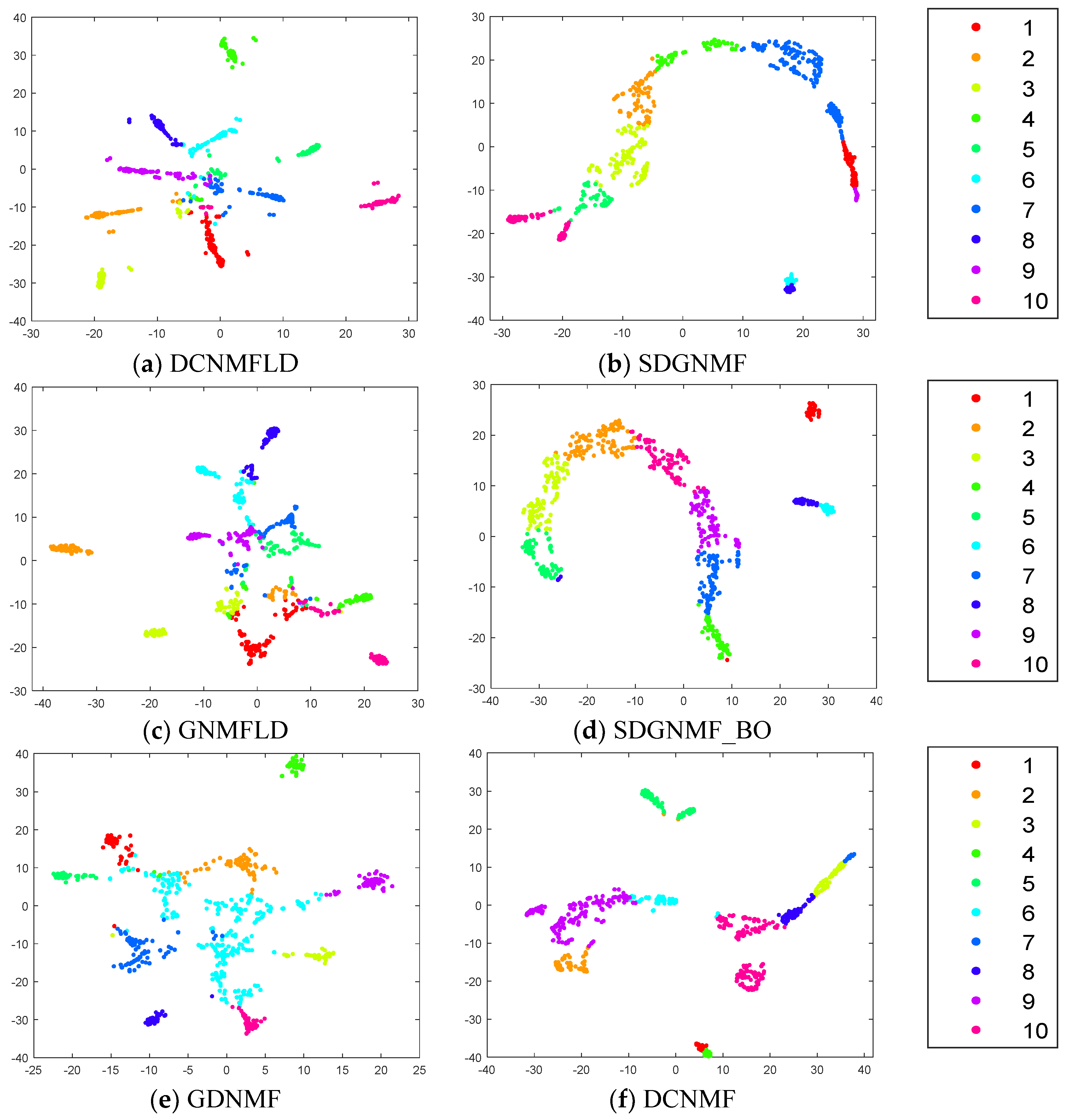
4.6. Visualization Comparison

To intuitively demonstrate the subspace learning proficiency of DCNMFLD, we utilize t-SNE to project the low-dimensional data, obtained from a variety of comparative algorithms on the YaleB dataset onto a two-dimensional plane. The outcomes of this visual comparison are illustrated in Figure 1. It can be observed from Figure 1 that the low-dimensional representation, as learned by the DCNMFLD algorithm, presents a more pronounced inter-class distance within the subspace. The visualization of this low-dimensional data not only strengthens the reliability of the previously mentioned clustering experimental results but also affirms that the inherent constraints in DCNMFLD can augment the learning potential of the computational subspace.

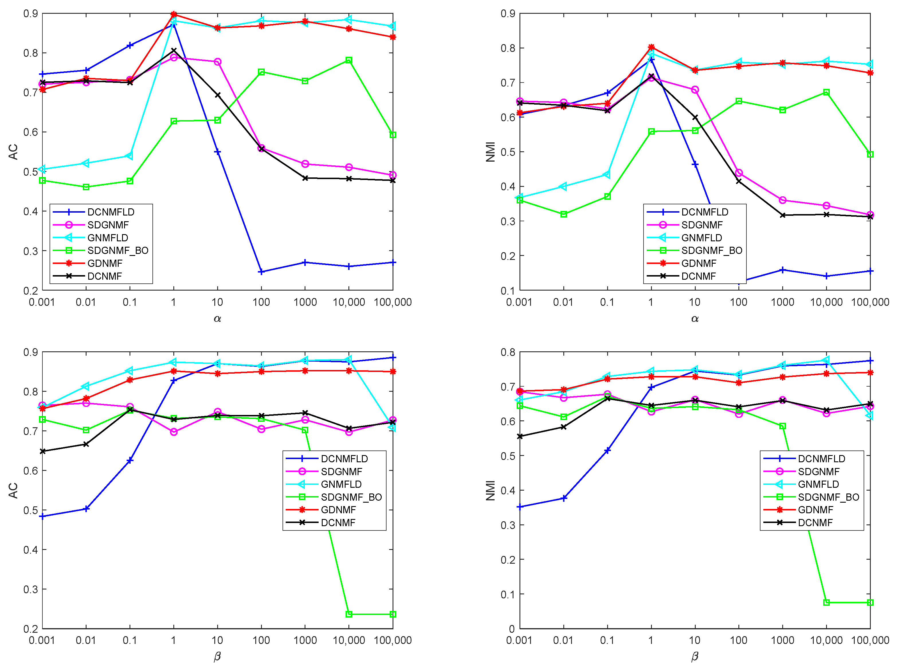
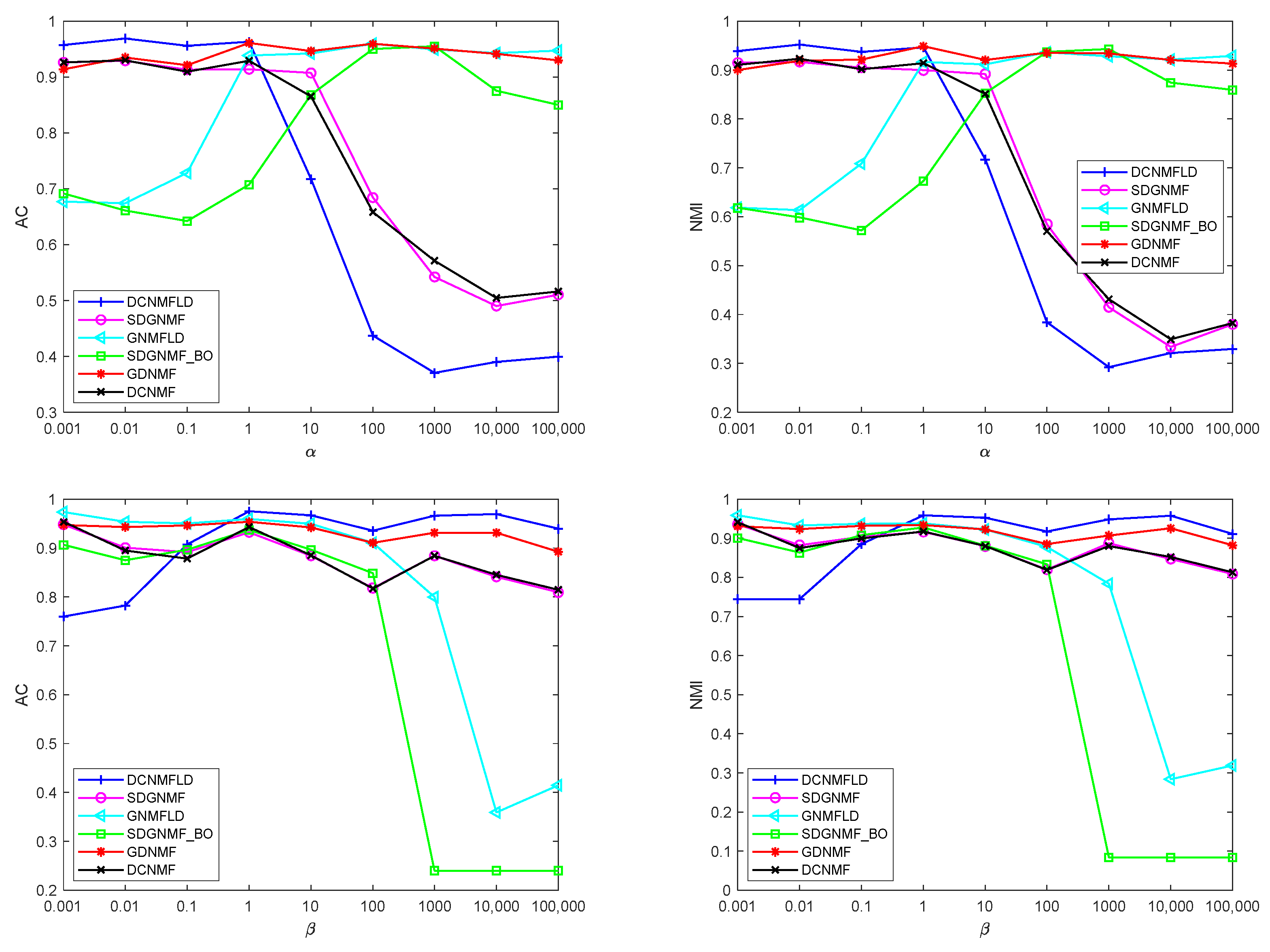
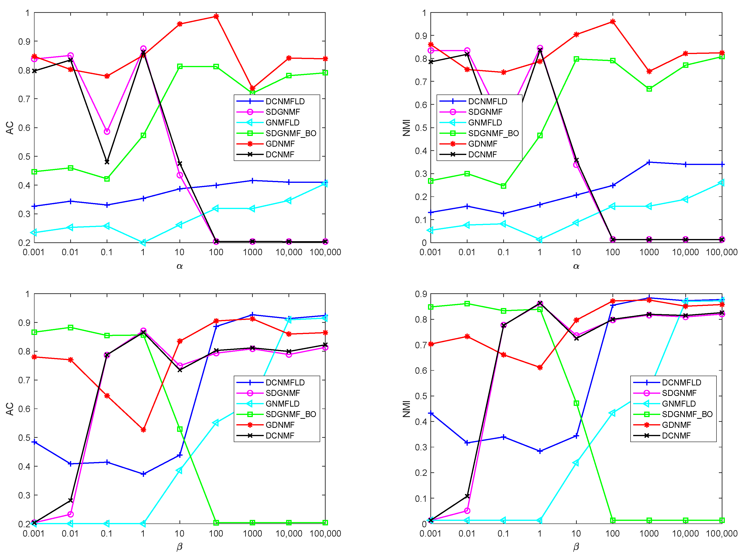
4.7. Parameter Selection

There are still other parameters that need to be set in the comparison method. Empirically, we set $\gamma$ as 10,000 in DCNMFLD for datasets YaleB and Isolet5, 0.01 for Jaffe and ORL, and 0.1 for dataset Yale. The sparse coefficient in SDFNMF is 0.6 for the ORL dataset, and 0.5 for other datasets. We adopt the grid search method to select the values of parameters α and β for comparison methods. Following previous works [22,30,34], we randomly selected five classes from each dataset for the experiments. Following the approach outlined in [36], we first empirically set β = 1 in all methods. We then proceeded to search for the optimal values of α within the range of [0.001, 0.01, 0.1, 1, 10, 100, 1000, 10,000, 100,000]. Once parameter α was fixed, we then searched for the optimal values of β also within the range of [0.001, 0.01, 0.1, 1, 10, 100, 1000, 10,000, 100,000]. Each experiment was repeated 20 times, and the average clustering performances are presented in Figure 2, Figure 3, Figure 4, Figure 5 and Figure 6. From Figure 2, Figure 3, Figure 4, Figure 5 and Figure 6, the values of parameters α and β that we set in clustering experiments are listed in

Table 9. Values of ($\alpha$, $\beta$) of the six methods on four datasets.

	DCNMFLD	SDGNMF	GNMFLD	SDGNMF_BO	GDNMF	DCNMF
Yale	(1, 100,000)	(1, 0.01)	(10,000, 10,000)	(10,000, 0.1)	(1, 1000)	(1, 0.1)
ORL	(0.01, 1)	(0.01, 0.001)	(100, 0.001)	(1000, 1)	(1, 1)	(0.01, 0.001)
Jaffe	(0.1, 1000)	(10, 1)	(1000, 1000)	(1000, 0.1)	(1000, 1000)	(1, 0.01)
YaleB	(10, 100)	(1, 10,000)	(100, 100)	(100,000, 0.01)	(10,000, 100)	(1, 100)
Isolet5	(1000, 1000)	(1, 1)	(100,000, 100,000)	(10, 0.01)	(100, 1000)	(1, 1)

.

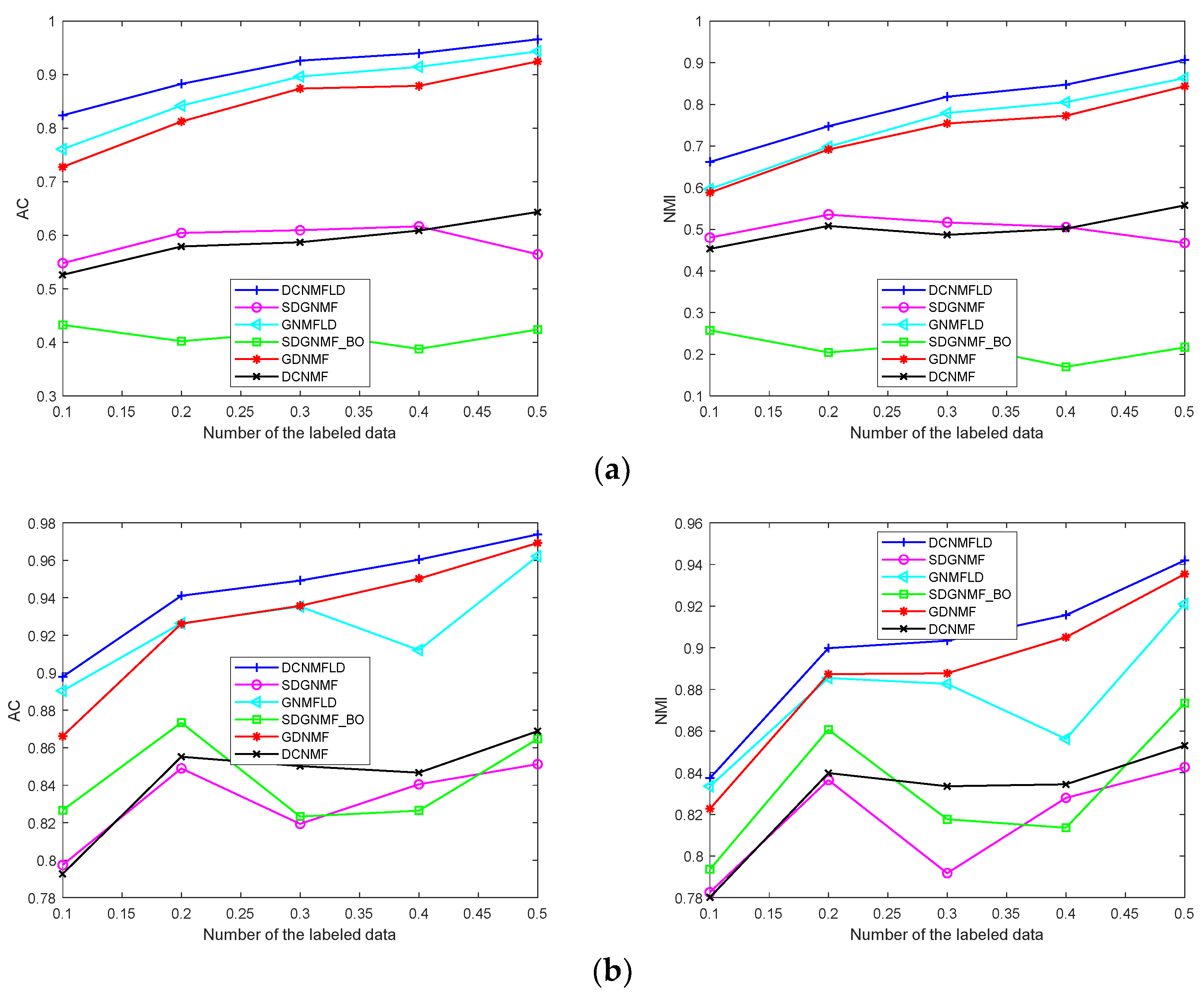
4.8. Relation with the Labeled Data Proportion

This study examined the impact of various semisupervised NMF algorithms on clustering performance under different proportions of labeled data points. Specifically, we randomly selected five clusters and varied the ratios of labeled data points (10%, 20%, 30%, 40%, and 50%) from each class for each dataset. We evaluated the average clustering outcomes of each algorithm across four datasets. The results shown in Figure 7 and Figure 8 indicate that as the number of labeled data points increases, the performance of the DCNMFLD algorithm also improves.

5. Conclusions

We introduced a semisupervised NMF method called DCNMFLD. DCNMFLD incorporated the label discrimination term of GNMFLD into the objective function of DCNMF [31]. This method aims to preserve the geometric information of both the data and feature spaces by constructing two p-nearest neighbor graphs that capture the manifold structure of data and feature space. Additionally, DCNMFLD can achieve a more discriminative representation. Experimental results demonstrated that DCNMFLD outperformed other state-of-the-art methods in terms of effectiveness and discriminative power. However, our method still has some shortcomings and areas for improvement. For example, compared to GNMFLD, DCNMF, and GDNMF, DCNMFLD has an additional regularization parameter that needs to be set, which undoubtedly poses difficulties in setting the value of regularization parameters. Although DCNMFLD integrates the feature graph, the clustering results on the Jaffe and ORL datasets show that the role of the feature graph is not obvious. In addition, using a feature graph will take more time during algorithm operation, which limits the application of DCNMFLD on ultra-high dimensional large datasets. In the future, drawing inspiration from other works [37,38], we want to extend DCNMFLD in multi-view tasks and design new regularization graphs to adapt to the characteristics of data.

References

1. Cai, D.; He, X.; Wu, X.; Han, J. Non-negative matrix factorization on manifold. In Proceedings of the 2008 Eighth IEEE International Conference on Data Mining, Pisa, Italy, 15–19 December 2008; pp. 63–72. [Google Scholar]
2. Lai, Z.; Xu, Y.; Chen, Q.; Yang, J.; Zhang, D. Multilinear sparse principal component analysis. IEEE Trans. Neural Netw. Learn. Syst. 2014, 25, 1942–1950. [Google Scholar] [CrossRef] [PubMed]
3. Lu, Y.; Lai, Z.; Xu, Y.; Li, X.; Yuan, C. Nonnegative discriminant matrix factorization. IEEE Trans. Circuits Syst. Video Technol. 2017, 27, 1392–1405. [Google Scholar] [CrossRef]
4. Kirby, M.; Sirovich, L. Application of the karhunen loeve procedure for the characterization of human faces. IEEE Trans. Pattern Anal. Mach. Intell. 1990, 12, 103–108. [Google Scholar] [CrossRef]
5. Dan, K. A singularly valuable decomposition: The svd of a matrix. Coll. Math. J. 1996, 27, 2–23. [Google Scholar]
6. Belhumeur, P.N.; Hespanha, J.; Kriegman, D.J. Eigenfaces vs fisher faces: Recognition using class specific linear projection. IEEE Trans. Pattern Anal. Mach. Intell. 1997, 19, 711–720. [Google Scholar] [CrossRef]
7. Xu, W.; Gong, Y. Document clustering by concept factorization. In Proceedings of the 27th Annual International ACM SIGIR Conference on Research and Development in INFORMATION Retrieval, SIGIR’04, Sheffield, UK, 25–29 July 2004; pp. 202–209. [Google Scholar]
8. Lee, D.D.; Seung, H.S. Learning the parts of objects by non-negative matrix factorization. Nature 1999, 401, 788–791. [Google Scholar] [CrossRef] [PubMed]
9. Lee, D.; Seung, H.S. Algorithms for non-negative matrix factorization. Adv. Neural Inf. Process. Syst. 2001, 13, 556–562. [Google Scholar]
10. Li, S.Z.; Hou, X.W.; Zhang, H.J.; Cheng, Q.S. Learning spatially localized, parts-based representation, In Proceedings of the 2001 IEEE Computer Society Conference on Computer Vision and Pattern Recognition. CVPR 2001, Kauai, HI, USA, 8–14 December 2001; pp. 207–212. [Google Scholar]
11. Xu, W.; Gong, Y. Document clustering based on non-negative matrix factorization. In Proceedings of the 26th Annual International ACM SIGIR Conference on Research and Development in Informaion Retrieval, SIGIR’03, Toronto, ON, Canada, 28 July–1 August 2003. [Google Scholar]
12. Shahnaz, F.; Berry, M.W.; Pauca, V.P.; Plemmons, R.J. Document clustering using nonnegative matrix factorization. Inf. Process. Manag. 2006, 42, 373–386. [Google Scholar] [CrossRef]
13. Kim, W.; Chen, B.; Kim, J.; Pan, Y.; Park, H. Sparse nonnegative matrix factorization for protein sequence motif discovery. Expert Syst. Appl. 2011, 38, 13198–13207. [Google Scholar] [CrossRef]
14. Shashua, A.; Hazan, T. Non-negative tensor factorization with applications to statistics and computer vision. In Proceedings of the 22nd International Conference on Machine Learning, Bonn, Germany, 7–11 August 2005; pp. 792–799. [Google Scholar]
15. Lu, N.; Miao, H. Structure constrained nonnegative matrix factorization for pattern clustering and classification. Neurocomputing 2016, 171, 400–411. [Google Scholar] [CrossRef]
16. Cai, D.; He, X.; Han, J. Document clustering using locality preserving indexing. IEEE Trans. Knowl. Data Eng. 2005, 17, 1624–1637. [Google Scholar] [CrossRef]
17. Kim, J.; Park, H. Sparse Nonnegative Matrix Factorization for Clustering. Available online: https://faculty.cc.gatech.edu/~hpark/papers/GT-CSE-08-01.pdf (accessed on 1 August 2023).
18. He, C.; Fei, X.; Cheng, Q.; Li, H.; Hu, Z.; Tang, Y. A survey of community detection in complex networks using nonnegative matrix factorization. IEEE Trans. Comput. Soc. Syst. 2021, 9, 440–457. [Google Scholar] [CrossRef]
19. Zhang, X.; Gao, H.; Li, G.; Zhao, J.; Huo, J.; Yin, J. Multi-view clustering based on graph-regularized nonnegative matrix factorization for object recognition. Inf. Sci. 2018, 432, 463–478. [Google Scholar] [CrossRef]
20. Wu, W.; Kwong, S.; Zhou, Y.; Jia, Y.; Gao, W. Nonnegative matrix factorization with mixed hypergraph regularization for community detection. Inf. Sci. 2018, 435, 263–281. [Google Scholar] [CrossRef]
21. Wang, J.Y.; Bensmail, H.; Gao, X. Multiple graph regularized nonnegative matrix factorization. Pattern Recognit. 2013, 46, 2840–2847. [Google Scholar] [CrossRef]
22. Cai, D.; He, X.; Han, J.; Huang, T. Graph regularized nonnegative matrix factorization for data representation. IEEE Trans. Pattern Anal. Mach. Intell. 2011, 33, 1548–1560. [Google Scholar]
23. Shang, F.; Jiao, L.; Wang, F. Graph dual regularization non-negative matrix factorization for co-clustering. Pattern Recognit. 2012, 45, 2237–2250. [Google Scholar] [CrossRef]
24. Belkin, M.; Niyogi, P.; Sindhwani, V. Manifold regularization: A geometric framework for learning from examples. J. Mach. Learn. Res. 2006, 7, 2399–2434. [Google Scholar]
25. Zhu, X.; Ghahramani, Z.; Lafferty, J.D. Semi-supervised learning using gaussian fields and harmonic functions. In Proceedings of the 20th International conference on Machine Learning (ICML-03), Washington, DC, USA, 21–24 August 2003. [Google Scholar]
26. Lee, H.; Yoo, J.; Choi, S. Semi-supervised nonnegative matrix factorization. IEEE Signal Process. Lett. 2010, 17, 4–7. [Google Scholar]
27. Liu, H.; Wu, Z.; Li, X.; Cai, D.; Huang, T.S. Constrained nonnegative matrix factorization for image representation. IEEE Trans. Pattern Anal. Mach. Intell. 2012, 34, 1299–1311. [Google Scholar] [CrossRef]
28. Babaee, M.; Tsoukalas, S.; Babaee, M.; Rigoll, G.; Datcu, M. Discriminative Nonnegative Matrix Factorization for dimensionality reduction. Neurocomputing 2015, 173, 212–223. [Google Scholar] [CrossRef]
29. Chen, P.; He, Y.; Lu, H.; Wu, L. Constrained Non-negative Matrix Factorization with Graph Laplacian. In Proceedings of the International Conference on Neural Information Processing: 22nd International Conference, ICONIP 2015, Istanbul, Turkey, 9–12 November 2015. [Google Scholar]
30. Li, H.; Zhang, J.; Shi, G.; Liu, J. Graph-based discriminative nonnegative matrix factorization with label information. Neurocomputing 2017, 266, 91–100. [Google Scholar] [CrossRef]
31. Sun, J.; Cai, X.; Sun, F.; Hong, R. Dual graph-regularized constrained nonnegative matrix factorization for image clustering. KSII Trans. Internet Inf. Syst. 2017, 11, 2607–2627. [Google Scholar]
32. Sun, J.; Wang, Z.; Sun, F.; Li, H. Sparse dual graph-regularized nmf for image co-clustering. Neurocomputing 2018, 316, 156–165. [Google Scholar] [CrossRef]
33. Li, S.T.; Li, W.G.; Hu, J.W.; Li, Y. Semi-supervised bi-orthogonal constraints dual-graph regularized nmf for subspace clustering. Appl. Intell. 2021, 52, 3227–3248. [Google Scholar] [CrossRef]
34. Xing, Z.; Ma, Y.; Yang, X.; Nie, F. Graph regularized nonnegative matrix factorization with label discrimination for data clustering. Neurocomputing 2021, 440, 297–309. [Google Scholar] [CrossRef]
35. Xing, Z.; Wen, M.; Peng, J.; Feng, J. Discriminative semi-supervised non-negative matrix factorization for data clustering. Eng. Appl. Artif. Intell. 2021, 103, 104289. [Google Scholar] [CrossRef]
36. Li, H.; Gao, Y.; Liu, J.; Zhang, J.; Li, C. Semi-supervised graph regularized nonnegative matrix factorization with local coordinate for image representation. Signal Process. Image Commun. 2022, 102, 116589. [Google Scholar] [CrossRef]
37. Dong, Y.; Che, H.; Leung, M.F.; Liu, C.; Yan, Z. Centric graph regularized log-norm sparse non-negative matrix factorization for multi-view clustering. Signal Process. 2024, 217, 109341. [Google Scholar] [CrossRef]
38. Liu, C.; Wu, S.; Li, R.; Jiang, D.; Wong, H.S. Self-Supervised Graph Completion for Incomplete Multi-View Clustering. IEEE Trans. Knowl. Data Eng. 2023, 35, 9394–9406. [Google Scholar] [CrossRef]
Figure 1. 2-D representations of YaleB dataset using t-SNE on the results of different methods.
Mathematics 12 00096 g001
Figure 2. The performance with the varied parameters α , β on the Yale dataset.
Mathematics 12 00096 g002
Figure 3. The performance with the varied parameter α , β on the ORL dataset.
Mathematics 12 00096 g003
Figure 4. The performance with the varied parameters α , β on the Jaffe dataset.
Mathematics 12 00096 g004
Figure 5. The performance with the varied parameters α , β on the YaleB dataset.
Mathematics 12 00096 g005
Figure 6. The performance with the varied parameters α , β on the Isolet5 dataset.
Mathematics 12 00096 g006
Figure 7. The performance with a varied number of the labeled data. (a) Yale, (b) ORL, and (c) Jaffe.
Mathematics 12 00096 g007
Figure 8. The performance with a varied number of the labeled data. (a) YaleB and (b) Isolet5.
Mathematics 12 00096 g008