Modified Unit-Half-Normal Distribution with Applications

Abstract

In this article, we introduce a new continuous distribution based on the unit interval. This distribution is generated from a transformation of a random variable with half-normal distribution. We study its basic properties, percentiles, moments and order statistics. Maximum likelihood estimation is applied, and we present a simulation study to observe the behavior of the maximum likelihood estimators. We examine two applications to real proportions datasets, where the new distribution is shown to provide a better fit than other distributions defined in the unit interval.

1. Introduction

In real life, it is quite common to find continuous data sets in the interval $(0,1)$. These data are the product of measurements that interpret different indices and rates. An example is insurance data, where a probability distribution can be used as a distortion function to define a premium principle (see Denuit et al. [1]). There are many studies involving measurements between $(0,1)$, see for example Cook et al. [2] and Gupta and Nadarajah [3], etc. Continuous distributions with support in $(0,1)$ are fundamental for modeling these data; for example, the two-parameter Beta is the model most frequently used to model data of this kind due to its great flexibility (see Johnson et al. [4]). A random variable (r.v.) X is called a Beta distribution with parameters $\alpha$ and $\beta$ if its probability density function (pdf) is given by

$$f_Z(z;\alpha ,\beta )=\frac{1}{B(\alpha ,\beta )}{z}^{\alpha -1}{(1-z)}^{\beta -1},0<z<1,$$

where $\alpha >0$, $\beta >0$ and B($·,·$) is the Beta function. Another distribution with support in $(0,1)$ is the Kumaraswamy distribution (see Kumaraswamy [5]). A r.v. Z has a Kumaraswamy (KM) distribution with parameters $\alpha$ and $\beta$ if its pdf is given by

$$f_Z(z;\alpha ,\beta )=\alpha \beta z^{\alpha -1}{(1-z^{\alpha })}^{\beta -1},0<z<1,$$

where $\alpha >0$ and $\beta >0$.

In recent years, several distributions with positive support have been transformed into distributions with unit support, for example Grassia [6], based on the Gamma distribution; Jones [7], based on the Kumaraswamy distribution; Mazucheli et al. [8], based on the Birnbaum-Saunders distribution; Ghitany et al. [9], based on the inverse Gaussian distribution; Modi et al. [10], based on the Burr III distribution; Korkmaz and Chesneau [11], based on the Burr XII distribution; Haq et al. [12], based on the modified Burr-III distribution; Gómez-Déniz et al. [13], Mazucheli et al. [14], Mazucheli et al. [15], based on the Lindley distribution, and more recently Bakouch et al. [16] based on the half-normal (HN) distribution. For example a distribution with support in $(0,1)$ and only one parameter is the unit-Lindley distribution (see Mazucheli et al. [14]). A r.v. Z is called a unit-Lindley (UL) distribution with parameter $\sigma$ if its pdf is given by

$$\begin{array}{c}\hfill f_Z(z;\sigma )=\frac{{\sigma }^2{(1-z)}^{-3}}{1+\sigma }exp\left(-\frac{\sigma z}{1-z}\right),0<z<1,\end{array}$$

where $\sigma >0$.

In this article, we introduce a new probability distribution with a restricted domain. Its distribution is derived by modifying the representation of the unit-half-normal (UHN) distribution introduced by Bakouch et al. [16]. One of the motivations of distribution theory is to provide new alternatives to known distributions in order to improve the statistical modeling of certain datasets. Our work is based on the HN distribution. Thus, we say that an r.v. X is called an HN distribution with scale parameter $\sigma$ if its pdf is given by

$$f_X(x;\sigma )=\frac{2}{\sigma }\varphi \left(\frac{x}{\sigma }\right),x>0,$$

with $\sigma >0$, and $\varphi (·)$ is the expression of the standard normal distribution. We denote this by $X\sim HN\left(\sigma \right)$ and some of its properties are:

• The cumulative distribution function (cdf) of X is $F_X(x;\sigma )=2\Phi \left(\frac{x}{\sigma }\right)-1.$
• The $r–$th moments are expressed by $E\left(X^r\right)=\frac{2^{r/2}\Gamma \left(\frac{r+1}{2}\right){\sigma }^r}{\sqrt{\pi }}$, $r=1,2,\dots$

where $\Phi (·)$ is the cdf of the standard normal distribution, and $\Gamma \left(x\right)={\int }_0^{\infty }{t}^{x-1}{e}^{-t}dt$ is the gamma function. Hogg and Tanis [17] discuss some properties of the HN distribution.

Bakouch et al. [16] introduce the UHN distribution, which is the product of a transformation of the random variables $X\sim HN\left(\sigma \right)$. Using the following transformation $Y=\frac{X}{1+X}$ they obtain the UHN distribution, the pdf of which is given by

$$f_Y(y;\sigma )=\frac{2}{\sigma {(1-y)}^2}\varphi \left(\frac{y}{\sigma (1-y)}\right),0<y<1,$$

(1)

where $\sigma >0$ and we denote it by $Y\sim UHN\left(\sigma \right)$.

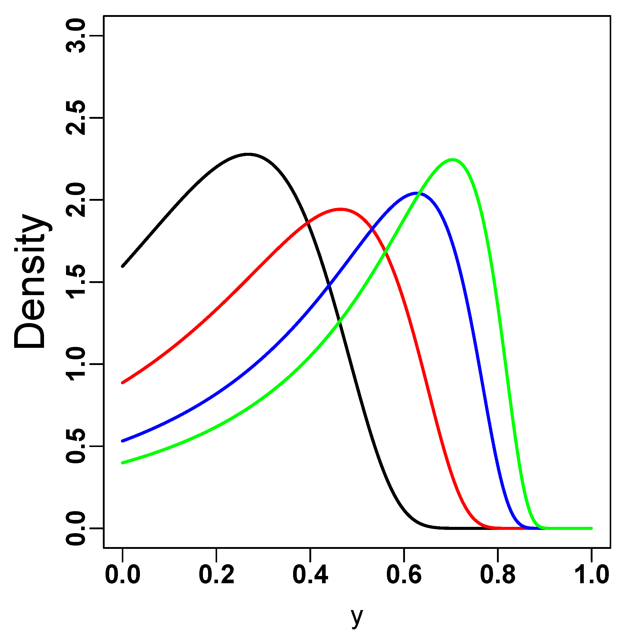
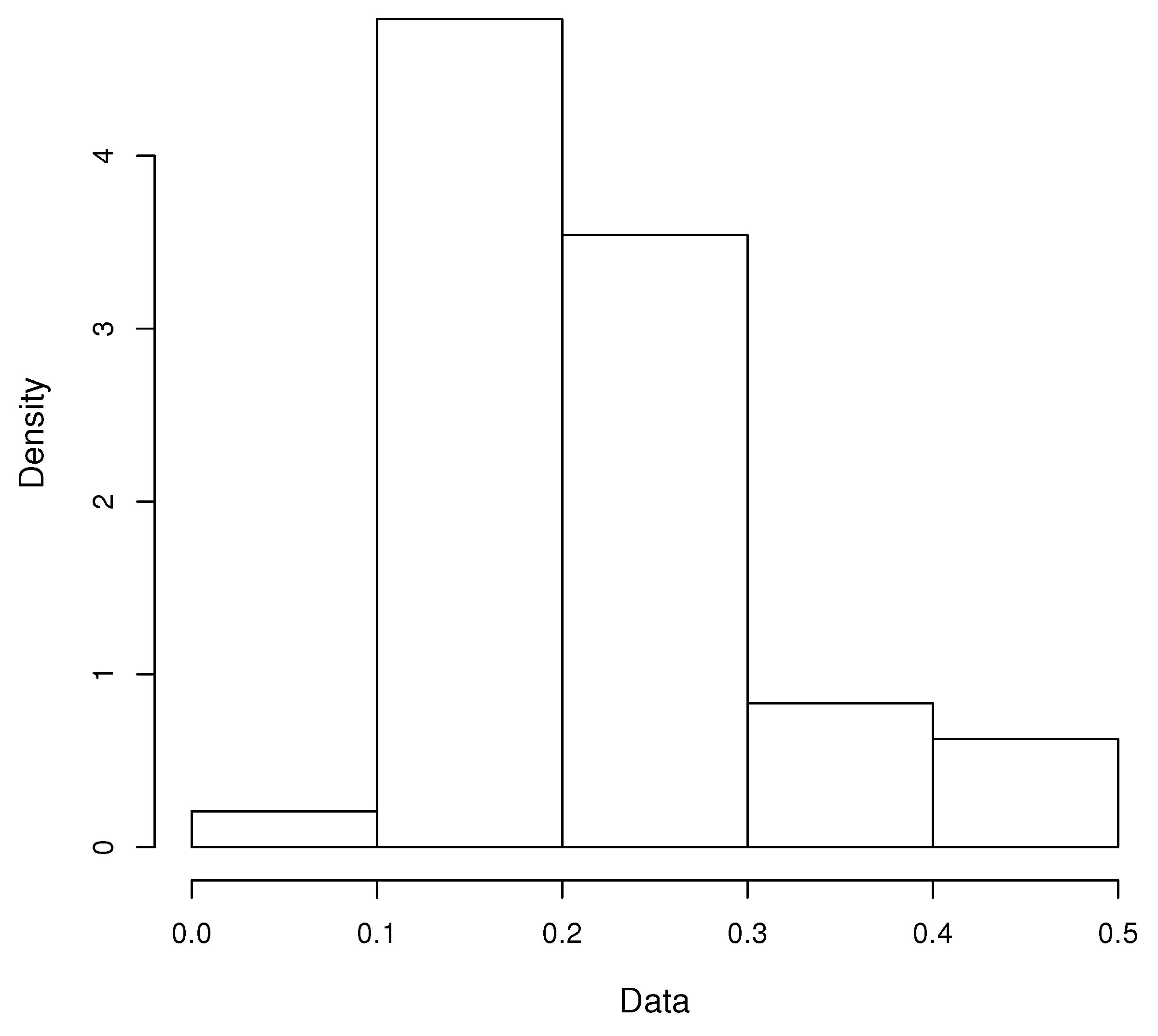
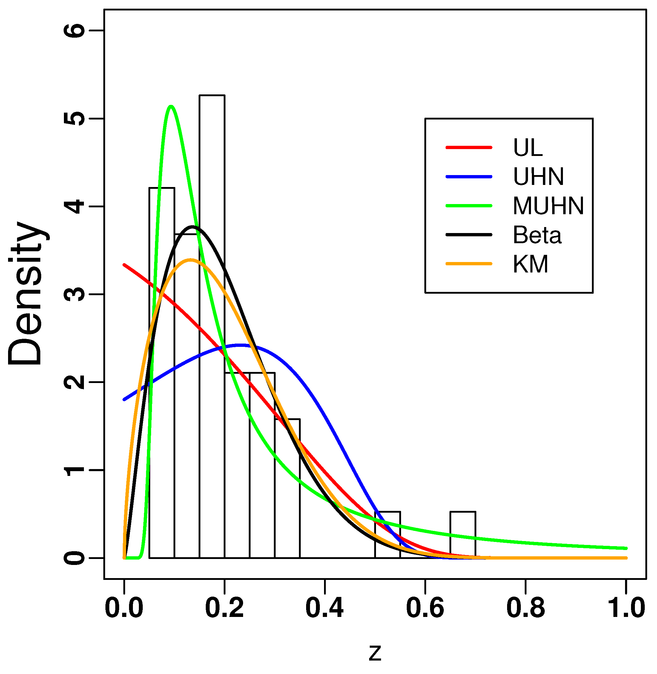
In Figure 1, we show the pdf of the UHN distribution for several values of $\sigma$. In Figure 2, we show a histogram of a proportions dataset. The shape that can be adopted by the UHN distribution close to zero does not represent this dataset; we therefore sought a different transformation with this characteristic. The main object of the present article is to study a new distribution that is a modification of the UHN distribution and offers an alternative to the UHN distribution for modeling proportion data with positive asymmetry, as shown by the data in Figure 2.

Figure 1. Densities UHN (0.5) (black), UHN (0.9) (red), UHN (1.5) (blue) and UHN (2) (green).

Figure 2. Histogram of a data set of proportions.

The rest of the paper is organized as follows. In Section 2, we give the representation of this distribution and generate the new density, its properties, moments and order statistics. In Section 3, we derive an inference by maximum likelihood (ML) and carry out a simulation study. Section 4 shows two applications to real datasets. In Section 5 we provide some final conclusions.

2. Density Function and Properties

In this section, we introduce the representation, density and properties of the new distribution.

2.1. Stochastic Representation

The representation of this new distribution is

$$Z=\frac{1}{1+X},$$

(2)

where $X\sim HN\left(\sigma \right)$, $\sigma >0$, and we call the distribution of Z the modified unit-half-normal (MUHN). This is denoted by $Z\sim MUHN\left(\sigma \right)$. Mazucheli et al. [15] use this representation in the Lindley distribution, obtaining a distribution called New Unit-Lindley (NUL). Applications of the NUL distribution are given in Ferreira and Mazucheli [18] and Alrumayh et al. [19], among others.

2.2. Density Function

The following result shows the pdf of the MUHN distribution, which is generated using the representation given in (2).

Proposition 1.

Let $Z\sim MUHN\left(\sigma \right)$. Then, the pdf of Z is given by

$$f_Z(z;\sigma )=\frac{2}{\sigma z^2}\varphi \left(\frac{1-z}{\sigma z}\right),0<z<1,$$

(3)

where $\sigma >0$.

Proof. 

Let $X\sim HN\left(\sigma \right)$, using the representation given in (2), and the random variables transformation method the result is obtained.    □

Proposition 2.

Let $Z\sim MUHN\left(\sigma \right)$. Then, the MUHN distribution has unimodality at $z_0=\frac{\sqrt{1+8{\sigma }^2}-1}{4{\sigma }^2}$.

Proof. 

Differentiating the density given in (3) with respect to z set equal to zero gives the result.    □

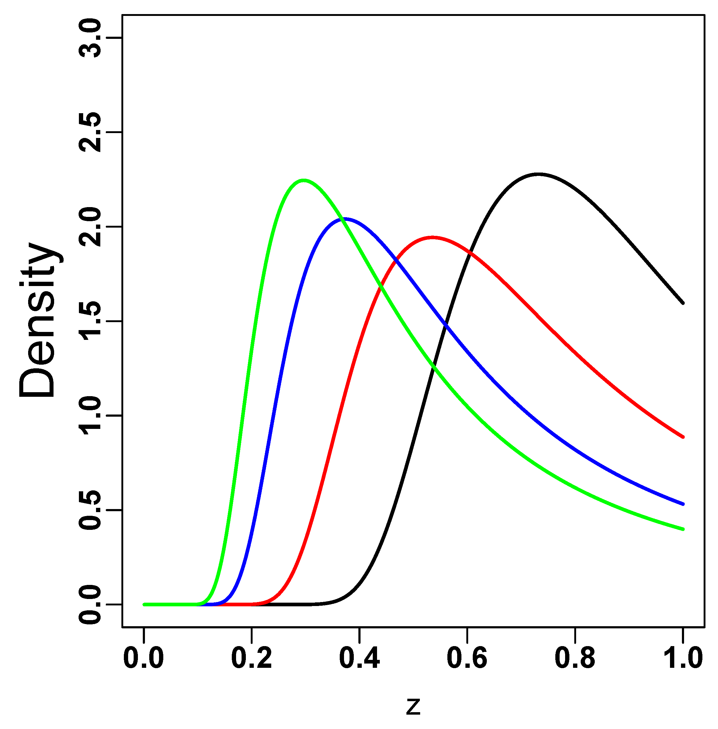
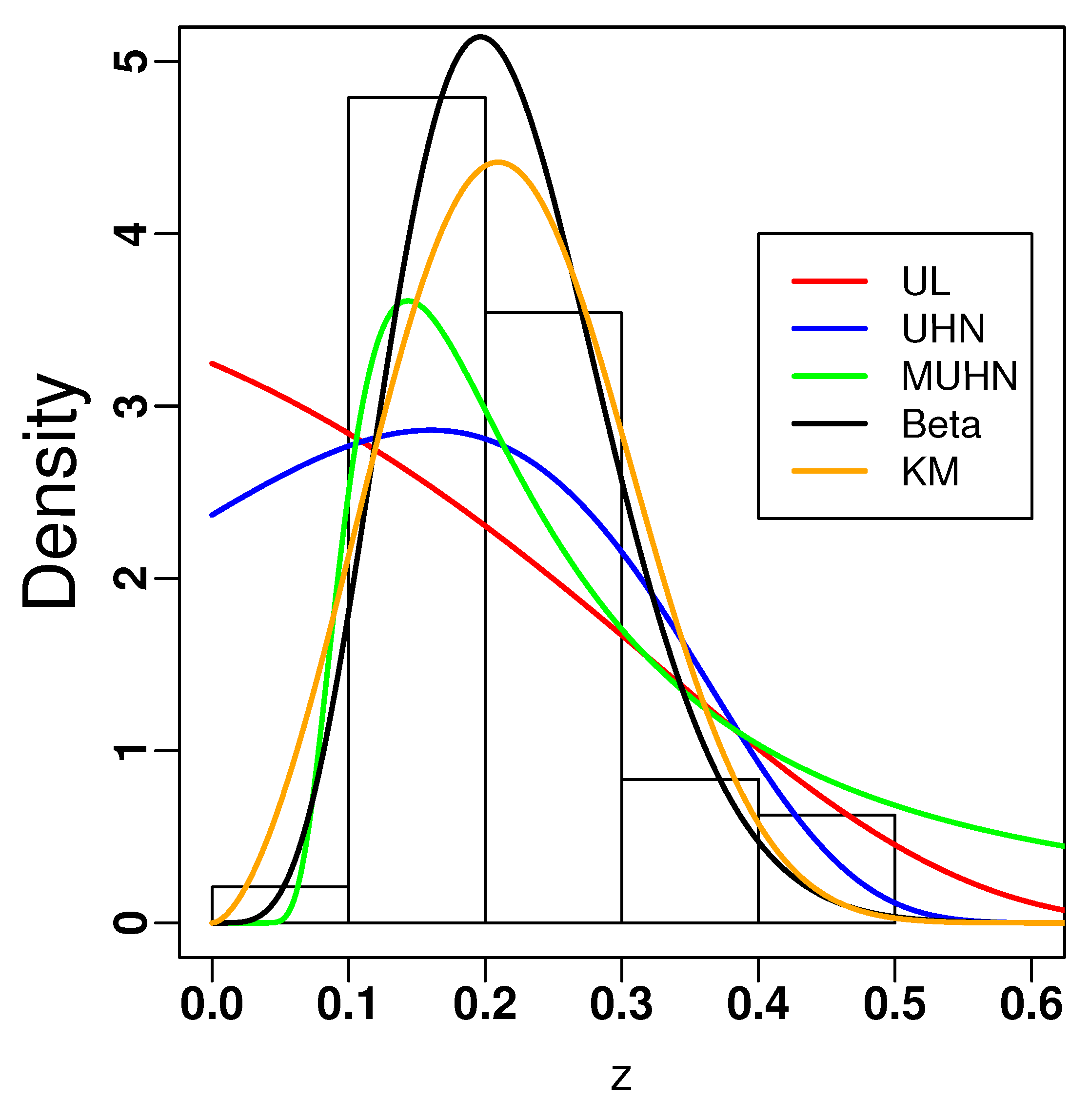
In Figure 3, we show the pdf of the MUHN distribution for several values of $\sigma$.

Figure 3. Densities MUHN (0.5) (black), MUHN (0.9) (red), MUHN (1.5) (blue) and MUHN (2) (green).

2.3. Cumulative Distribution Function

The following proposition shows the cdf of the MUHN distribution.

Proposition 3.

Let $Z\sim MUHN\left(\sigma \right)$. Then, the cdf of Z is given by

$$F_Z(z;\sigma )=2\Phi \left(\frac{z-1}{\sigma z}\right),$$

(4)

where $\sigma >0$.

Proof. 

Calculating the cdf of Z directly, we have

$${\displaystyle F_Z(z;\sigma )={\int }_0^z\frac{2}{\sigma t^2}\varphi \left(\frac{1-t}{\sigma t}\right)dt.}$$

Making the following change of the variable $u=\frac{1-t}{\sigma t}$, the result is obtained.    □

2.4. Reliability Analysis

The reliability function $r\left(t\right)$ and the hazard function $h\left(t\right)$ of the MUHN distribution are given in the following corollary.

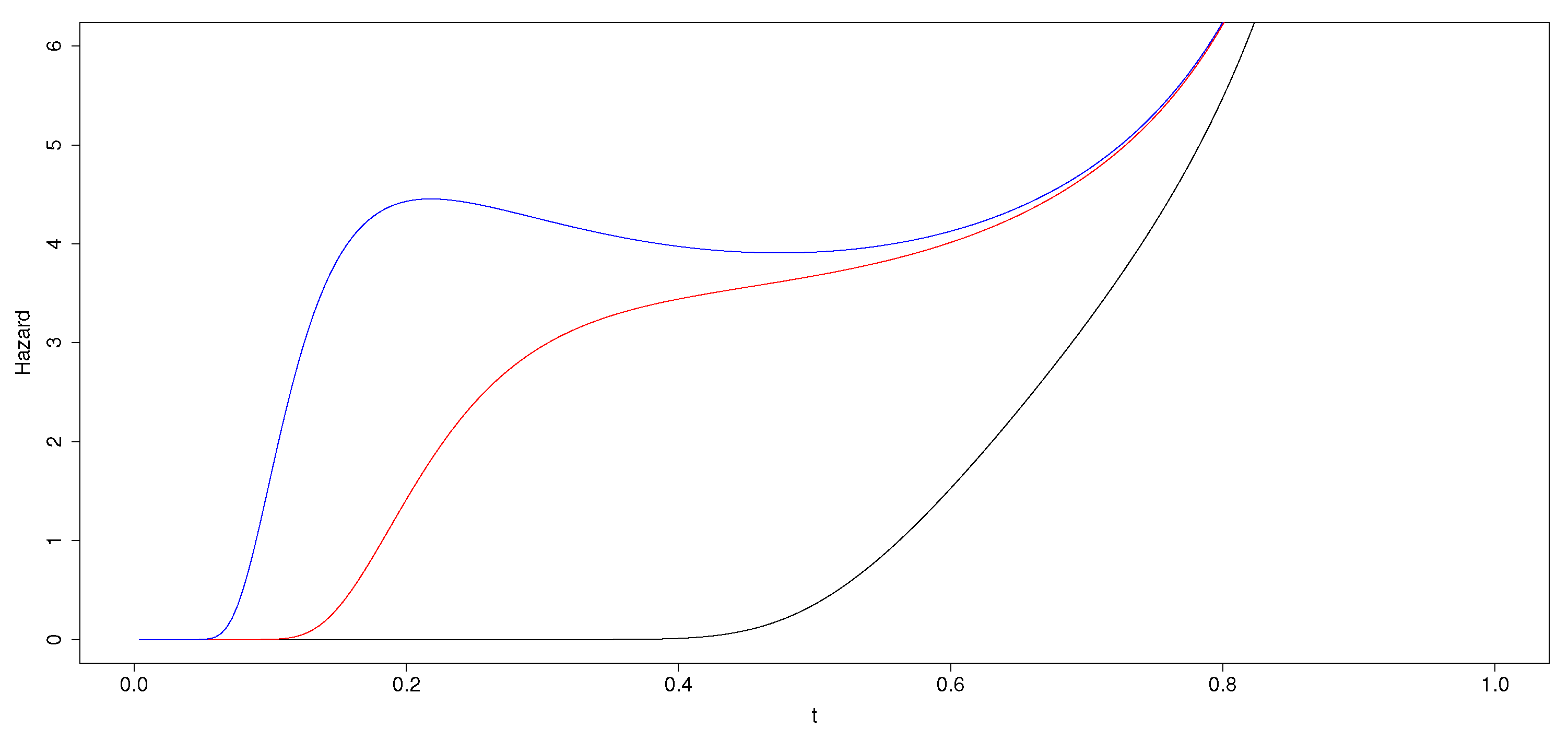
Corollary 1.

Let $T\sim MUHN\left(\sigma \right)$. Then, the reliability and hazard of T is given by

$$r\left(t\right)=1-2\Phi \left(\frac{t-1}{\sigma t}\right),andh\left(t\right)=\frac{2\varphi \left(\frac{1-t}{\sigma t}\right)}{\sigma t^2\left(1-2\Phi \left(\frac{t-1}{\sigma t}\right)\right)},$$

where $\sigma >0$ is shape parameter.

In Figure 4, we show the Hazard function of MUHN distribution for several values of $\sigma$.

Figure 4. Hazard function of MUHN distribution for selected values of $\sigma$: $\sigma =0.4$ (black), $\sigma =2$ (red) and $\sigma =4$ (blue).

Proposition 4.

Let $Z\sim MUHN\left(\sigma \right)$. Then, the quantile function (Q) of the MUHN distribution is given by

$$\begin{array}{c}\hfill Q\left(p\right)={\left\{1-\sigma {\Phi }^{-1}\left(\frac{p}{2}\right)\right\}}^{-1},0<p<1,\end{array}$$

(5)

where ${\Phi }^{-1}(·)$ is the inverse cdf of a standard normal distribution.

Proof. 

Using the cdf given in (4), we have

$$\begin{array}{c}\hfill p=F_Z(z;\sigma )=2\Phi \left(\frac{z-1}{\sigma z}\right).\end{array}$$

Applying the inverse function of the cdf of a standard normal distribution and clearing for z, the result is obtained.    □

2.5. Order Statistics

Let $Z_1,...,Z_n$ be a random sample of the r.v. $Z\sim MUHN\left(\sigma \right)$. We denote by $Z_{\left(j\right)}$ the $jth–$order statistics, $j\in \{1,\dots ,n\}$.

Proposition 5.

The pdf of $Z_{\left(j\right)}$ is

$$\begin{array}{c}\hfill f_{Z_{\left(j\right)}}(z;\sigma )={\displaystyle \frac{2^{j}n!}{\sigma (j-1)!(n-j)!z^2}}\varphi \left(\frac{1-z}{\sigma z}\right){\Phi }^{j-1}\left(\frac{z-1}{\sigma z}\right){\left[1-2\Phi \left(\frac{z-1}{\sigma z}\right)\right]}^{n-j},0<z<1.\end{array}$$

In particular, the pdf of the minimum, $Z_{\left(1\right)}$, is

$$f_{Z_{\left(1\right)}}(z;\sigma )=\frac{2n}{\sigma z^2}\varphi \left(\frac{1-z}{\sigma z}\right){\left[1-2\Phi \left(\frac{z-1}{\sigma z}\right)\right]}^{n-1},0<z<1$$

(6)

and the pdf of the maximum, $Z_{\left(n\right)}$, is

$$f_{Z_{\left(n\right)}}(z;\sigma )=\frac{n{2}^n}{\sigma z^2}\varphi \left(\frac{1-z}{\sigma z}\right){\Phi }^{n-1}\left(\frac{z-1}{\sigma z}\right),0<z<1$$

Proof. 

Since the model is absolutely continuous, the pdf of the $jth–$order statistics is obtained by applying

$$\begin{array}{ccc}\hfill f_{Z_{\left(j\right)}}(z;\sigma )& =& {\displaystyle \frac{n!}{(j-1)!(n-j)!}}{f}_Z(z;\sigma ){\left[F_Z(z;\sigma )\right]}^{j-1}{[1-F_Z(z;\sigma )]}^{n-j},j\in \{1,\dots ,n\}\hfill \end{array}$$

where F and f denote the cdf and pdf of the parent distribution, $Z\sim MUHN\left(\sigma \right)$ in this case.    □

2.6. Moments

An important numerical function for calculating the r-th moments of the random variable $Z\sim MUHN\left(\sigma \right)$ is defined as

$$a_r\left(\sigma \right)={\int }_0^{\infty }\frac{exp(-u^2/2)}{{(1+\sigma u)}^r}du,r=1,2,3,...$$

(7)

More details of this function can be found in Appendix A.

Proposition 6.

Let $Z\sim MUHN\left(\sigma \right)$. Then, for $r=1,2,3,\dots ,$ the r-th moment of Z is given by

$$\mathbb{E}\left(Z^r\right)=\frac{2}{\sqrt{2\pi }}{a}_r\left(\sigma \right).$$

(8)

Proof. 

Using the representation given in (2) and calculating the r-th moments directly, we have

$$\mathbb{E}\left(Z^r\right)=\mathbb{E}\left(\frac{1}{{(1+X)}^r}\right)={\int }_0^{\infty }\frac{2}{\sigma {(1+x)}^r}\varphi \left(\frac{x}{\sigma }\right)dx.$$

Making the following change in the variable $u=\frac{x}{\sigma }$, the result is obtained.    □

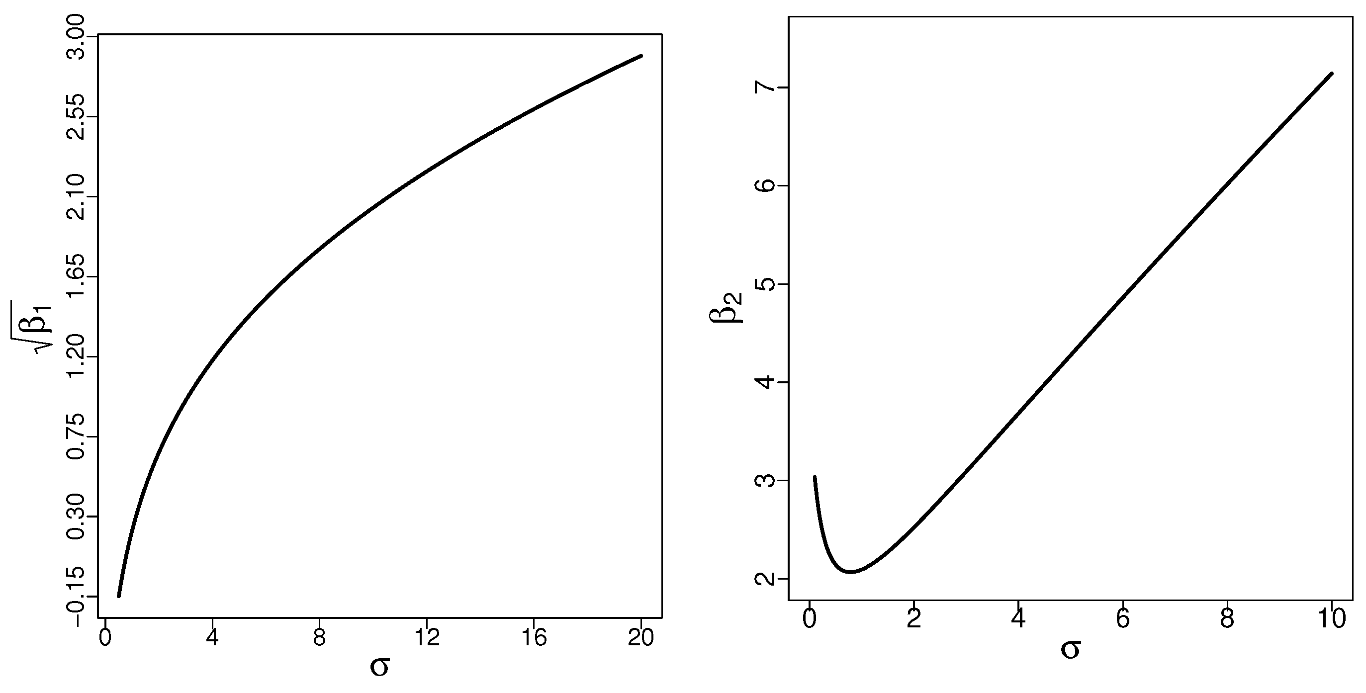
Corollary 2.

Let $Z\sim MUHN\left(\sigma \right)$. Then, the mean and variance of the r.v. Z are given respectively by

$$\begin{array}{c}\hfill {\displaystyle \mathbb{E}\left(Z\right)=2a_1\left(\sigma \right)\mathrm{and}Var\left(Z\right)=2\left(a_2\left(\sigma \right)-2a_1^2\left(\sigma \right)\right),}\end{array}$$

and the asymmetry and kurtosis coefficients are given respectively by

$$\sqrt{{\beta }_1}=\frac{a_3\left(\sigma \right)-6a_1\left(\sigma \right)a_2\left(\sigma \right)+8a_1^3\left(\sigma \right)}{\sqrt{2}{\left[a_2\left(\sigma \right)-2a_1^2\left(\sigma \right)\right]}^{3/2}},$$

$${\beta }_2=\frac{a_4\left(\sigma \right)-8a_1\left(\sigma \right)a_3\left(\sigma \right)+24a_1^2\left(\sigma \right)a_2\left(\sigma \right)-24a_1^4\left(\sigma \right)}{2{\left[a_2\left(\sigma \right)-2a_1^2\left(\sigma \right)\right]}^2}.$$

Figure 5 depicts plots for the asymmetry and kurtosis coefficients in the MUHN distribution.

Figure 5. Plots of the asymmetry and kurtosis coefficients for the MUHN model.

Proposition 7.

Let $Z\sim MUHN\left(\sigma \right)$. Then, the moment-generating function ($M_Z$) of the r.v. Z is given by

$$M_Z\left(t\right)=2\sum _{j=0}^{\infty }\frac{t^j}{j!}{a}_j\left(\sigma \right),$$

(9)

where $a_j$ are given in (7).

Proof. 

Using the representation given in (2), we have

$$M_Z\left(t\right)=\mathbb{E}\left(exp\left(tZ\right)\right)=\mathbb{E}\left(exp\left(\frac{t}{1+X}\right)\right)={\int }_0^{\infty }exp\left(\frac{t}{1+x}\right)\frac{2}{\sigma }\varphi \left(\frac{x}{\sigma }\right)dx,$$

making the change of the variable $u=\frac{x}{\sigma }$, expanding the $exp(·)$ function in series and using (7) the result is obtained.    □

The following proposition shows a closed expression for negative moments.

Proposition 8.

Let $Z\sim MUHN\left(\sigma \right)$. Then, for $r=1,2,3,\dots ,$ the negative r-th moment of Z is given by

$$\mathbb{E}\left(Z^{-r}\right)=\frac{{\sigma }^k}{\sqrt{\pi }}\sum _{k=0}^r\left(\genfrac{}{}{0pt}{}{r}{k}\right)2^{\frac{k}{2}}\Gamma \left(\frac{k+1}{2}\right).$$

(10)

Proof. 

Calculating the negative moments directly using binomial theorem, the result is obtained.    □

From this we have that: $\mathbb{E}\left(Z^{-1}\right)=1+\sigma \sqrt{\frac{2}{\pi }}.$

3. Inference

In this section, we estimate the parameter $\sigma$ of the MUHN model using a modified moments (MM) method and the ML method, we present a simulation study, and we discuss the asymptotic estimation of the ML estimator.

3.1. Mm Estimation

For a random sample $z_1,\dots ,z_n$ derived from the MUHN($\sigma$) distribution, $\overline{Z^{-1}}=\frac{1}{n}{\sum }_{i=1}^n\frac{1}{z_i}$, then MM estimator of $\sigma$ is:

$${\widehat{\sigma }}_{MM}=\sqrt{\frac{\pi }{2}}\left(\overline{Z^{-1}}-1\right).$$

(11)

3.2. Ml Estimation

For a random sample $z_1,\dots ,z_n$ derived from the MUHN($\sigma$) distribution, the log-likelihood function can be written as

$$\mathcal{l}\left(\sigma \right)=nlog\left(2\right)-nlog\left(\sqrt{2\pi }\right)-nlog\left(\sigma \right)-\sum _{i=1}^{n}log\left(z_i^2\right)-\frac{1}{2{\sigma }^2}\sum _{i=1}^n{\left(\frac{1-z_i}{z_i}\right)}^2.$$

(12)

The score equation is given by

$$\begin{array}{c}\hfill \frac{d\mathcal{l}\left(\sigma \right)}{d\sigma }=-\frac{n}{\sigma }+\frac{1}{{\sigma }^3}\sum _{i=1}^n{\left(\frac{1-z_i}{z_i}\right)}^2=0,\end{array}$$

(13)

the ML estimator for $\sigma$ ($\widehat{\sigma }$) is obtained by resolving the following Equation (13) and its

$$\begin{array}{c}\hfill \hat{\sigma }={\left\{\frac{1}{n}\sum _{i=1}^n{\left(\frac{1-z_i}{z_i}\right)}^2\right\}}^{1/2},\end{array}$$

(14)

Hence, for large samples, the ML estimator, $\widehat{\sigma }$, is asymptotically normal, that is,

$$\sqrt{n}\left(\widehat{\sigma }-\sigma \right)\stackrel{\mathcal{L}}{⟶}N(0,I_F^{-1}\left(\sigma \right)).$$

It results from this that the asymptotic variance of the ML estimator $\widehat{\sigma }$ is the inverse of Fisher’s information $I_F\left(\sigma \right)=\frac{2}{{\sigma }^2}$, i.e., $Var\left(\widehat{\sigma }\right)\approx \frac{{\sigma }^2}{2n}.$

Proposition 9.

For a random sample $z_1,\dots ,z_n$ derived from the MUHN(σ) distribution, we have that

$$\frac{\sqrt{n}}{\sigma }\widehat{\sigma }\sim {\chi }_{\left(n\right)}$$

(15)

where ${\chi }_{\left(n\right)}$ denotes the chi-distribution with n degrees of freedom.

Proof. 

As $Z\sim MUHN\left(\sigma \right)$, then $\frac{1}{{\sigma }^2}{\left(\frac{1-Z}{Z}\right)}^2\sim {\chi }_{\left(1\right)}^2$, where ${\chi }_{\left(1\right)}^2$ chi-squared distribution with 1 degree of freedom. From the properties of the chi-squared distribution we have $\frac{1}{{\sigma }^2}{\sum }_{i=1}^n{\left(\frac{1-z_i}{z_i}\right)}^2\sim {\chi }_{\left(n\right)}^2$, luego $\frac{\sqrt{n}}{\sigma }{\left\{\frac{1}{n}{\sum }_{i=1}^n{\left(\frac{1-z_i}{z_i}\right)}^2\right\}}^{1/2}\sim {\chi }_{\left(n\right)}$.    □

Corollary 3.

Some direct consequences of the result given in (15) are

• $\mathbb{E}\left(\widehat{\sigma }\right)=\frac{\sigma \sqrt{2}\Gamma \left(\frac{n+1}{2}\right)}{\sqrt{n}\Gamma \left(\frac{n}{2}\right)}$
• $Var\left(\widehat{\sigma }\right)={\sigma }^2\left(1-\frac{2{\Gamma }^2\left(\frac{n+1}{2}\right)}{n{\Gamma }^2\left(\frac{n}{2}\right)}\right)$

The $\widehat{\sigma }$ estimator is asymptotically unbiased for $\sigma$. With these results the bias and the mean squared error can be calculated.

3.3. Simulation Study

To examine the behavior of the ML estimation approach, we carried out a simulation study to assess the performance of the estimation, using the parameter $\sigma$ of the MUHN distribution. Two algorithms, Algorithms 1 and 2, are proposed to generate random numbers from the MUHN distribution. The simulation analysis was carried out by generating 1000 samples of size n = 30, 38, 40, 50, 80 and 100 from the MUHN distribution. The objective of this simulation is to study the behavior of the ML of the parameter $\sigma$ of the MUHN model.

Algorithm 1 to simulate values from the $Z\sim MUHN\left(\sigma \right)$ distribution.

1: Generate $Y\sim Uniform(0,1).$ 2: Compute $Z={\left\{1-\sigma {\Phi }^{-1}\left(\frac{Y}{2}\right)\right\}}^{-1}$.

Algorithm 2 to simulate values from the $Z\sim MUHN\left(\sigma \right)$ distribution.

1: Generate $Y\sim N(0,1)$. 2: Compute $X=\sigma \mid Y\mid$. 3: Compute $Z=\frac{1}{1+X}$.

The code for both algorithms can be found in the following repository https://github.com/isaaccortes1989/MUHN-Codes (accessed on 2 November 2023). Since the results of the two algorithms are similar, we only present those of Algorithm 1. Table 1 displays the empirical bias (B), standard deviation (SD), mean of the standard errors (SEs), root of the empirical mean squared error (RMSE), and the coverage probability (CP). The CP terms converge reasonably to the nominal value used for their construction (95%), suggesting that the normality is reasonable for the asymptotic distribution of the ML estimators in the MUHN model. As shown in Table 1, the performance of the estimations improves as n increases.

Table 1. ML estimates, B, SD, SE, RMSE, and CP for the MUHN model with sample size 30, 38, 40, 50, 80 and 100, respectively.

$\mathit{\sigma }$	n	$\widehat{\mathit{\sigma }}$	B	SD	SE	RMSE	CP
0.5	30	0.496	−0.008	0.065	0.064	0.065	0.936
	38	0.498	−0.003	0.058	0.057	0.058	0.941
	40	0.499	−0.003	0.056	0.056	0.056	0.954
	50	0.499	−0.002	0.050	0.050	0.050	0.937
	80	0.500	0.000	0.038	0.040	0.038	0.959
	100	0.501	0.001	0.035	0.035	0.035	0.949
1	30	0.987	−0.013	0.127	0.127	0.128	0.926
	38	0.989	−0.011	0.111	0.113	0.112	0.934
	40	0.991	−0.009	0.108	0.111	0.108	0.944
	50	0.995	−0.005	0.097	0.099	0.097	0.937
	80	0.996	−0.004	0.079	0.079	0.079	0.938
	100	0.997	−0.003	0.068	0.070	0.068	0.950
1.5	30	1.487	−0.009	0.189	0.192	0.190	0.932
	38	1.489	−0.007	0.169	0.171	0.169	0.943
	40	1.489	−0.007	0.167	0.166	0.168	0.936
	50	1.492	−0.005	0.149	0.149	0.149	0.943
	80	1.495	−0.004	0.114	0.118	0.114	0.950
	100	1.496	−0.003	0.104	0.106	0.104	0.949
2	30	1.967	−0.016	0.250	0.254	0.252	0.927
	38	1.974	−0.013	0.224	0.226	0.225	0.938
	40	1.973	−0.014	0.221	0.221	0.222	0.928
	50	1.981	−0.010	0.195	0.198	0.196	0.928
	80	1.990	−0.005	0.158	0.157	0.158	0.944
	100	1.991	−0.005	0.138	0.141	0.138	0.950
2.5	30	2.495	−0.002	0.327	0.322	0.327	0.934
	38	2.489	−0.004	0.292	0.286	0.292	0.933
	40	2.489	−0.004	0.283	0.278	0.283	0.941
	50	2.494	−0.002	0.253	0.249	0.253	0.937
	80	2.498	−0.001	0.191	0.197	0.191	0.949
	100	2.498	−0.001	0.171	0.177	0.171	0.951
3	30	2.972	−0.009	0.376	0.384	0.377	0.943
	38	2.975	−0.008	0.338	0.341	0.339	0.934
	40	2.977	−0.008	0.330	0.333	0.331	0.943
	50	2.988	−0.004	0.300	0.299	0.300	0.940
	80	2.988	−0.004	0.231	0.236	0.231	0.944
	100	2.990	−0.003	0.213	0.211	0.213	0.946
4	30	3.960	−0.010	0.529	0.511	0.530	0.918
	38	3.963	−0.009	0.459	0.455	0.460	0.933
	40	3.969	−0.008	0.448	0.444	0.449	0.936
	50	3.980	−0.005	0.403	0.398	0.403	0.937
	80	3.989	−0.003	0.320	0.315	0.320	0.940
	100	3.993	−0.002	0.282	0.282	0.282	0.947
5	30	4.949	−0.010	0.647	0.639	0.648	0.927
	38	4.958	−0.008	0.580	0.569	0.581	0.929
	40	4.968	−0.006	0.560	0.555	0.560	0.926
	50	4.973	−0.005	0.509	0.497	0.510	0.938
	80	4.987	−0.003	0.398	0.394	0.398	0.938
	100	4.988	−0.002	0.348	0.353	0.348	0.951
7.2	30	7.149	−0.007	0.930	0.923	0.931	0.939
	38	7.164	−0.005	0.836	0.822	0.836	0.939
	40	7.166	−0.005	0.813	0.801	0.813	0.939
	50	7.171	−0.004	0.743	0.717	0.743	0.922
	80	7.175	−0.003	0.584	0.567	0.585	0.94
	100	7.173	−0.004	0.526	0.507	0.526	0.936

4. Applications

This section shows two applications of the MUHN model, highlighting its superior performance compared to other models known in the statistical literature.

4.1. Application 1

In this first application, we fit the MUHN distribution and compare it with the uniparametric UL and UHN distributions and the two-parameter Beta and KM distributions defined in the Introduction. The dataset consists of 48 samples of rocks from an oil reservoir, as reported by Cordeiro and Brito [20]. We conducted an analysis of the shape perimeter using a squared variable (area). The data are in Table 2:

Table 2. The data of 48 samples of rocks from an oil reservoir.

0.0903296	0.2036540	0.2043140	0.2808870	0.1976530	0.3286410
0.1486220	0.1623940	0.2627270	0.1794550	0.3266350	0.2300810
0.1833120	0.1509440	0.2000710	0.1918020	0.1541920	0.4641250
0.1170630	0.1481410	0.1448100	0.1330830	0.2760160	0.4204770
0.1224170	0.2285950	0.1138520	0.2252140	0.1769690	0.2007440
0.1670450	0.2316230	0.2910290	0.3412730	0.4387120	0.2626510
0.1896510	0.1725670	0.2400770	0.3116460	0.1635860	0.1824530
0.1641270	0.1534810	0.1618650	0.2760160	0.2538320	0.2004470

Table 3 displays basic descriptive statistics for the dataset. We employ the notation $\sqrt{b_1}$ and $b_2$ to denote sample asymmetry and kurtosis coefficients, respectively.

Table 3. Descriptive statistics for the first dataset.

Data Set	n	$\overline{\mathit{Z}}$	S	$\sqrt{{\mathit{b}}_1}$	${\mathit{b}}_2$
Rock samples from a petroleum reservoir	48	$0.218$	$0.083$	$1.169$	$4.110$

Using Section 3.1, the MM estimator of $\sigma$ is ${\widehat{\sigma }}_{MM}=5.258.$

Table 4 shows the parameters estimated by ML for the UL, UHN, MUHN, Beta and KM models. Standard errors of the ML estimates are calculated using Fisher’s information corresponding to each model. For each model, we report the values of the Akaike information criterion (AIC), introduced by Akaike [21], and the Bayesian information criterion (BIC), proposed by Schwarz [22]. It is observed that both AIC and BIC criteria indicate a better fit for the Beta model.

Table 4. Parameter estimates with SEs (in parentheses), AIC and BIC values for UL, UHN, MUHN, Beta and KM models.

Parameter Estimates	UL	UHN	MUHN	Beta	KM
$\alpha$	-	-	-	5.942 (1.181)	2.719 (0.294)
$\beta$	-	-	-	21.206 (4.347)	44.661 (17.576)
$\sigma$	$4.049\left(0.502\right)$	$0.337\left(0.035\right)$	$4.565\left(0.466\right)$	-	-
AIC	$-68.700$	$-81.053$	$-87.316$	$-107.200$	$-100.983$
BIC	$-66.829$	$-79.182$	$-85.445$	$-103.458$	$-97.241$

Figure 6 illustrates the ML fit of the five models with the probability histogram. Additionally, we calculate the quantile residuals (QRs). If the model is suitable for the data, the QRs should be a sample from the standard normal model (see Dunn and Smyth [23]). This assumption can be validated using traditional normality tests, such as the Anderson–Darling (AD), Cramér-von Mises (CVM) and Shapiro–Wilkes (SW) tests.

Figure 6. Histogram for rock samples from a petroleum reservoir; lines represent distributions fitted using ML estimates: UL$\left(\widehat{\sigma }\right)$ (red), UHN$\left(\widehat{\sigma }\right)$ (blue), MUHN$\left(\widehat{\sigma }\right)$ (green), Beta$(\widehat{\alpha },\widehat{\beta })$ (black) and KM$(\widehat{\alpha },\widehat{\beta })$ (brown).

In Figure 7, the QRs for the fitted models and the p-values for the AD, CVM and SW normality tests are provided to assess whether the QRs follow the standard normal distribution. It is observed that the QRs follow the standard normal distribution only for the MUHN model; in other word, all three test show that the data did not come from the UL, UHN, Beta and KM distributions. Figure 7 suggest that the MUHN model gives a better fit for this dataset.

Figure 7. QQ-plots of the QRs: UL distribution (a); UHN distribution (b); MUHN distribution (c); Beta distribution (d) and KM distribution (e).

The codes for this application are available on the following website: https://github.com/isaaccortes1989/MUHN-Codes/tree/main/First%20Application (accessed on 2 November 2023).

4.2. Application 2

In this second application, we fit the MUHN distribution and compare it with the two-parameter Beta and KM distributions that are defined in the Introduction. The data set consists of a sample of 38 proportions formed by COVID information taken from the Chilean database, from 4 March to 10 April 2020. These data were formed using new cases (NC), daily accumulated cases (AC) and daily cumulative deaths (CD). We analyze the proportion of daily NC to the accumulated number of survivors with the equation:

$$z_i=\frac{N{C}_i}{A{C}_i-C{D}_{i-1}}.$$

The data are in Table 5.

Table 5. The data of a sample of 38 proportions formed by COVID information.

0.666666667	0.25	0.2	0.285714286	0.3
0.333333333	0.117647059	0.260869565	0.303030303	0.23255814
0.295081967	0.186666667	0.519230769	0.223880597	0.155462185
0.304093567	0.211981567	0.191806331	0.150316456	0.152815013
0.190889371	0.192644483	0.125574273	0.188819876	0.156626506
0.107526882	0.126582278	0.105551497	0.096667766	0.109576968
0.089108911	0.101898582	0.069335719	0.071443406	0.058835027
0.077533357	0.071332887	0.081372097

Table 6 shows the descriptive summary of the data, highlighting their positive asymmetry. Using Section 3.1, the MM estimator of $\sigma$ is ${\widehat{\sigma }}_{MM}=7.656.$

Table 6. Descriptive statistics for the second dataset.

Data Set	n	$\overline{\mathit{Z}}$	S	$\sqrt{{\mathit{b}}_1}$	${\mathit{b}}_2$
COVID	38	0.194	0.125	1.863	7.347

The estimates, SE, AIC, and BIC values for the UL, UHN, KM, Beta and MUHN models are displayed in Table 7. From the table, it is evident that the MUHN model demonstrates a better fit, as it exhibits the smallest criteria values with only one parameter. Furthermore, the fit of the five models with the histogram of the data can be observed in Figure 8, confirming the better fit of the MUHN model. Finally, as shown in Figure 9, all QRs indicate that a standard normal distribution is followed only for the MUHN model.

Table 7. Parameter estimates with their respective SE (in parentheses), AIC and BIC values for the indicated model.

Parameter Estimates	UL	UHN	KM	Beta	MUHN
$\alpha$	-	-	1.610 (0.211)	2.325 (0.501)	-
$\beta$	-	-	10.512 (3.368)	9.438 (2.205)	-
$\sigma$	4.141 (0.578)	0.443 (0.051)	-	-	7.231 (0.829)
AIC	−51.442	−39.916	−58.371	−61.191	−67.334
BIC	−49.805	−38.278	−55.096	−57.916	−65.696

Figure 8. Histogram for COVID dataset; lines represent distributions fitted using ML estimates.

Figure 9. QQ-plots of the QRs: KM distribution (a); Beta distribution (b); MUHN distribution (c); UL distribution (d) and UHN distribution (e).

The codes for this application are available on the following website: https://github.com/isaaccortes1989/MUHN-Codes/tree/main/Second%20Application (accessed on 2 November 2023).

5. Discussion

This paper presents a study of the MUHN distribution. We show some properties and compare them with the UHN distribution in a fit using ML estimation. The MUHN distribution appears to be a viable alternative for fitting data between zero and one, and with positive asymmetry. Some other characteristics of the MUHN distribution are:

• The representation of the MUHN distribution is simple.
• The MUHN distribution has an explicit mode.
• The cdf, hazard function and quantile function are explicit and represented by known functions.
• The ML estimator shows very good behavior with small samples.
• The applications show that the MUHN distribution is a very good alternative when the data present positive asymmetry; this was confirmed by both the AIC and BIC model selection criteria and by the Anderson–Darling, Cramér-von Mises and Shapiro–Wilkes statistical tests.