Abstract
This paper proposes a Kalman filter for linear rectangular singular discrete-time systems, where the singular matrix in the system is a rectangular matrix without full column rank. By using two different restricted equivalent transformation methods and adding the measurement equation to the state equation, the system is transformed into a square singular system satisfying regularity and observability. During this process, the causality of the system is taken into account, and multiple matrix transformations are applied accordingly. Based on these modifications, state estimation results are obtained using the Kalman filter. Finally, a numerical example is employed to demonstrate the effectiveness of our approach.
MSC:
94A12
1. Introduction
State estimation has always been an important topic in practical applications. Since the least squares method was proposed, many state estimation methods for linear systems have been proposed [1,2,3,4,5]. Among these, the Kalman filter [6] is the optimal state estimation method for linear Gaussian systems. Therefore, many advanced Kalman filters have been proposed, and these studies have achieved good filtering effects [7,8,9,10], which provide many theoretical references for singular systems.
Singular systems, also known as descriptor systems, were first proposed by Rosenbrock in 1974 to address power grid systems [11]. The remarkable characteristic of the system is that there may be a singular matrix in the dynamic space equation of the system. Compared to regular systems, singular systems can represent physical systems better than regular ones and have important applications in circuit systems, chemical systems and economic systems [12,13]. Thus, there are many contributions based on singular systems [14,15]. In singular systems, some properties are similar to regular systems, such as stability, controllability, observability, and detectability [16]. However, an important difference between singular systems and regular systems is that singular systems may be impulsive. As a result, research on singular systems is more complex compared to regular systems.
The state estimation problem of singular systems has attracted widespread attention due to its application background. The state estimation methods for linear discrete singular systems mainly include reduced-order estimation methods based on singular value decomposition (SVD), maximum likelihood method, least squares method and minimum variance estimation method [17]. Apart from these methods, many state estimation methods for singular systems under different situations have also been proposed. Liu et al. considered the estimation problem of discrete-time linear fractional-order singular systems [18,19]. Yu discussed the singular systems with multiplicative noise using the restricted equivalent transformation method and recursive Riccati equation [20,21]. Zhang proposed an optimal recursive filtering method for singular random discrete systems based on the ARMA innovation model and time-domain innovation analysis method [22]. Zhang [23] investigates the positive real lemmas for singular fractional-order linear time-invariant systems. In addition, there are many studies on the causality, controllability, stability, regular performance perception, and stabilization of singular systems, which further improve the theories of singular systems [24,25,26,27].
However, most of the research is aimed at square matrix singular systems, and many conclusions about square matrix systems can not be applied when the singular matrix is a rectangular matrix. One of the facts is that only square systems have regularity [28]. Zhang et al. [29] extended the regularity of square matrix singular systems to non-square singular systems, proposed the concept of generalized regularity, and gave the corresponding necessary and sufficient conditions. The necessary and sufficient conditions show that when the matrix array is not full rank, the solution of the system is not unique. Therefore, the state estimation problem of rectangular systems without full column rank must satisfy the premise that the whole system is observable. For the problem of state estimation of rectangular singular systems, Tian [30] decomposes the restricted equivalent transformation of the system equation into two parts by means of singular value decomposition when the system is regular and strongly controllable, and then he uses the generalized inverse theory to transform the singular system into the problem of state estimation of normal systems. However, this paper only considers the case that the singular matrix of the transformed equation is full column rank. Wen [31] proposed a method for decomposing the state using QR decomposition theory, which does not assume that the singular matrix has full rank, and extended the problem to time-varying situations, but did not consider the system’s impulsive nature.
In discrete singular systems, the impulse property of the system is the causality of the system. If the rectangular singular system is a noncausal system, the state value of the system will be related to future information, and the existence of this characteristic will affect the estimation of the system state value. However, to my knowledge, existing state estimation methods for linear rectangular singular systems have not taken into account the causal properties of the system. Therefore, the main contribution of this paper is to propose a state estimation method for linear rectangular singular systems considering noncausal situations, providing a new approach for the state estimation problem of rectangular singular systems. The main work of this paper is: two restricted equivalent transformations were applied to the system, followed by multiple matrix transformations based on the causality of the system. Additionally, a portion of the measurement equation is incorporated into the state equation to transform the system into a non-singular one. Based on these modifications, optimal state estimation results are obtained using the Kalman filter method. Finally, the effectiveness of the proposed method is validated through numerical examples.
The remaining sections of this paper are arranged as follows: Section 2 presents the problems to be addressed and the corresponding assumptions, Section 3 applies a series of system transformations to convert the system into a non-singular form, Section 4 outlines the state estimation method based on the Kalman filter, Section 5 provides numerical simulations, and Section 6 concludes the paper.
Notations. The notations throughout this paper are fairly standard except specifically stated. and denote the n-dimensional Euclidean space and the set of all matrices, respectively. The superscript and represent the transposition and the inverse one of matrix X, respectively. denotes the n-dimensional identity matrix and denotes matrix whose elements are all zeros. is the expectation of random variable w and is the rank of matrix M. and denote the prediction and estimation of state , respectively. and denote the prediction error covariance and estimation error covariance of a state at instant k, respectively. For , denotes the matrix M is composed of elements , and the element in the ith row and jth column of matrix M is . denotes z is a complex number, where denotes a complex domain.
2. Problem Formulation
Consider a discrete-time linear singular system:
where . The matrix E is a singular matrix and , , , , , , , are zero-mean Gaussian noise. The system satisfies the following assumptions:
Assumption 1.
where is the Kronecker function.
Assumption 2.
There exists a complex such that [32].
Assumption 3.
The system is observable and [29]:
In this paper, the estimation of will be obtained by systems (1) and (2) based on measurements .
3. System Transformation Based on Constrained Equivalence Transformation
In this section, we will sequentially perform two different constrained equivalence transformations on the system. In this process, a part of the observation equation will be combined with the state equation, so that the state equation becomes a square system that satisfies the regularity and observability of square singular matrices. Finally, the system will be transformed into a system that can be estimated using state estimation methods for square singular systems. Therefore, in this section, we first introduce the two constrained equivalence transformation methods that will be used.
3.1. Two Constrained Equivalence Transformation Methods
3.1.1. The First Type of Restricted Equivalent Transformation
For the matrix E in Equation (1), there exists an orthogonal matrix such that matrix E can be decomposed according to its singular values as:
where, , , and . represents the non-zero singular values of matrix E. We perform the corresponding matrix transformation on the state x and let , . . Equation (1) transforms to:
3.1.2. The Second Type of Restricted Equivalent Transformation
Consider a square singular system:
where, , , , is zero-mean Gaussian noise.
For the matrix pair , there exists an orthogonal matrix such that:
where , , represents the determinant of the target matrix, represents the order of the target determinant, thus . is a nilpotent matrix, and , . In this paper, we refer to the degree of the nilpotent matrix ℵ as b.
We perform the corresponding matrix transformation on the state and let , . . Equation (4) transforms to:
Let , Equation (5) can be split into:
Equations (6) and (8) are the restricted equivalent systems transformed from (1) through the second type of restricted equivalent transformation.
If the system is a non-causal system, when the first type of restricted equivalent transformation method is used to transform the system, the transformed system cannot highlight the non-causality. However, using the second type of restricted equivalent transformation method can highlight the non-causality of the system. In addition, the principle of the first type of restricted equivalent transformation method is relatively simple, so causal singular systems are suitable for using the first type of restricted equivalent transformation method for transformation, and non-causal singular systems are suitable for using the second type of restricted equivalent transformation method for transformation.
3.2. The System Transformation Based on Constrained Equivalence Transformation
We have obtained Equation (3) through the first type of restricted equivalent transformation. Let , Equation (3) can be decomposed into:
where, .
Theorem 1.
The matrix is a row full rank matrix.
Proof.
According to Assumption 2, , and both matrix U and matrix V are orthogonal matrices. Recall when a matrix is multiplied by an invertible matrix, the rank of the matrix remains unchanged. Therefore, we have:
Therefore, is full row rank, which means that . Thus, the matrix is a matrix with full row rank. □
Equation (9) can be transformed into:
Substituting , into Equation (2), it transforms into:
Lemma 1.
The constrained equivalence transformation method does not change the observability of the system.
Matrix U and matrix V are both orthogonal matrices, Therefore:
Therefore, the system formed by Equations (3) and (13) is still observable.
According to Equation (14) and given , The matrix is composed of at least linearly independent row vectors to ensure that . Without losing generality, these row vectors come from the first rows of matrix , which is denoted as , , then we have:
Let , , , , .
Theorem 2.
Matrix is an invertible matrix.
Proof.
According to Equation (15), . Where is a diagonal matrix. Thus, elementary transformations can be performed on matrix as:
Therefore, . Thus we can conclude that given .
Therefore, Matrix is an invertible matrix. □
Theorem 3.
In matrix , there exist at least row vectors, denoted as , such that .
Proof.
According to Theorem 2, . According to Theorem 1, .
The equivalent proposition of Theorem 3 is: There are at least row vectors in the matrix that cannot be linearly represented by the row vectors of matrix . Assuming its converse proposition holds true: at most () row vectors in the matrix cannot be linearly represented by the row vectors of matrix . The equivalent proposition of the converse proposition is: There are at least l row vectors in the matrix that can be linearly represented by the row vectors of the matrix . Based on the equivalent proposition of the converse proposition and , we have:
Equation (19) contradicts . Therefore, there are at least row vectors in the matrix that cannot be linearly represented by the row vectors of matrix , which means there exist at least row vectors, denoted as , in matrix such that:
□
Without losing generality, matrix comes from the first rows of matrix . Correspondingly, the first rows of are denoted as , . Based on Theorem 3, we can infer:
Matrix is a part of , thus, let , , , , . Based on , Equation (17) can be rewritten as:
and Equation (21) can be divided into two parts:
Combining Equations (7) and (19):
where, , . Let .
Theorem 4.
Equation (25) is regular, in other words, there exists a complex number , such that .
Proof.
According to , is a row full rank matrix. Therefore, regardless of the value of matrix , there exists a complex number , such that:
According to Theorem 3, , which means is a row full rank matrix. Therefore, regardless of the value of matrix , there exists a complex number , such that:
According Equation (11):
In summary, regardless of the value of , there exists a complex number , such that:
Therefore, . □
Combining Equations (18) and (23), we have:
Let , , , , , Equations (25) and (26) can be rewritten as follows, respectively:
Theorem 5.
.
Proof.
The following equation holds:
Therefore:
□
According to Theorems 4 and 5, the system composed of Equations (27) and (28) is observable and regular.
According to the second type of restricted equivalent transformation, there exist orthogonal matrixes , , such that:
where, , , , is a nilpotent matrix with degree h. Let , , Equation (27) can be transformed into:
Let , Equation (30) can be divided into two parts:
From Equation (32), we have:
Substituting , into Equation (23):
Equation (33) contains the unknown term at the current time, . This prevents us from estimating the system state based on the current information. Therefore, further transformations are needed to convert the system into a known system that does not include unknown terms.
3.3. Transforming the System into a Known System
In Section 3.2, after performing a constrained equivalence transformation on the system, we obtained a system composed of Equations (3) and (13). Then, we combined a part of the observation equation with the state equation and performed a second constrained equivalence transformation, resulting in a system composed of Equations (31), (33) and (34). In this chapter, we will transform the system into a known system by a series of transformations that eliminate the unknown terms.
Performing a simple row transformation on Equation (25):
In Equation (35), matrices and are both rectangular matrices with more columns than rows. We can rewrite both matrices as a combination of a square matrix and several column vectors:
If we perform the second type of constrained equivalence transformation on the matrix pair , transformation matrices can be denoted as and , respectively. Let , matrix and can be transformed into:
where, , , , . is a nilpotent matrix with degree . Let:
For the nilpotent matrix , all of its eigenvalues are 0. Therefore, if matrix transforms into a Jordan matrix, all the diagonal elements of the Jordan matrix are 0. Consequently, there exists an invertible matrix such that can be transformed into a Jordan matrix as follows, denoted as :
The degree of matrix is , thus in Equation (38), the first rows contain the number 1.
Left multiplying matrix and by matrix , and right multiplying them by :
Let , Expanding and , we obtain:
In Equation (41), all elements in rows to are zeros. Therefore, We perform the same elementary column transformations on the matrix blocks and , respectively:
Denoting the final results of Equations (43) and (44) as a combination of a square matrix and several column vectors:
where, , noting that matrix is non-invertible.
If we perform the second type of constrained equivalence transformation on matrices and , transformation matrices can be denoted as and , respectively. Matrix and can be transformed as follows:
where, , , , . is a nilpotent matrix with degree .
The matrix blocks and in Equation (37) have undergone the following transformations through Equations (37)–(48), where the entire process consists of elementary transformations or multiplication with invertible matrices:
Applying a similar transformation process as in Equations (37)–(48) on the matrix blocks and in Equation (49), we can obtain an expression similar to Equation (49):
We refer to Equation (49) as the first transformation and Equation (50) as the second transformation, then the result of the ith transformation is:
where, , . When the tth transformation results in or , there will be two situations.
If , the degree of matrix at this point is , and Equation (36) finally transforms into:
If , Equation (36) finally transforms into:
If the transformation takes the form of Equation (52), it indicates that the system is non-causal. If it transforms into Equation (53), it indicates that the system is causal. Let .
The block matrix and in Equation (52) can be transformed similar to Equations (38), and we denote the transformation matrix as . The result of Equation (52) can be further transformed as follows:
where, matrix is similar in form to Equation (38) and can be denoted as follows:
In Equation (55), the first row vectors of matrix contain the number 1.
Taking the non-causal system represented by Equations (52) and (54) as an example, since the entire transformation process represented by Equations (52) and (54) is a sequence of elementary transformations or multiplication by invertible matrices, the entire process can be viewed as left multiplying by an invertible matrix and right multiplying by another invertible matrix. Let us denote the left multiplication matrix as , the right multiplication matrix as , and let . Then, Equation (35) can be transformed into:
Let , , , , , , , , substituting these into Equation (56) gives:
In Equation (57), may not be an invertible matrix, which may result in the presence of unknown terms similar to Equation (33) in subsequent transformations of Equation (57). Therefore, theorem 6 is given to solve this problem.
Theorem 6.
In matrix , there exist row vectors, denoted as , such that when matrix undergoes the right multiplication transformation described in Equation (58) (equivalent to a column transformation), the resulting matrix is invertible.
where, , , .
Proof.
Let:
Left multiplying matrix and by matrix , and right multiplying them by , we obtain:
From Equation (15) we know that:
The transformation in Equation (59) does not change the rank of , thus we can observe the following from Equation (59):
Therefore, matrix is invertible, and all column vectors of matrix are linearly independent. Hence, there exist at least linearly independent row vectors in matrix , denoted as matrix , and we can infer that matrix is invertible. Similarly, we denote matrix , which comes from matrix , as the matrix corresponding to matrix . □
Let , , replace and with and , respectively, Equation (57) can be rewritten as:
Based on , let . Since row vectors have been selected from matrix to replace , the observation Equation (28) is correspondingly rewritten as:
where, .
The system formed by Equations (61) and (62) is still regular and observable (the proof process is similar to Theorems 4 and 5).
Equations (1) and (2) undergo a series of transformations and are ultimately transformed into Equations (61) and (62). During this process, before adding the measurement equation to the state equation, all transformations involving the measurement equation are column transformations. In other words, the measurement noises are not fused with each other. Therefore, the noises in Equation (61) and the noises in Equation (62) do not have a correlation. Therefore, the classical Kalman filter can be used for systems (61) and (62).
Through the transformations and decompositions from Equations (36)–(61), the entire system becomes a solvable known system that does not contain unknown terms at the current time. For causal systems represented by Equation (53), the transformation process is similar to that of non-causal systems, and can also obtain a solvable known system. Therefore, in subsequent analysis, we will mainly focus on non-causal systems represented by Equation (52). Next, we will perform state estimation on the system in a form similar to standard Kalman filtering.
4. Filtering Algorithm
4.1. One-Step Prediction
From Equation (30), we can obtain Equations (31) and (33). Similarly, let , from Equation (64) we can obtain the following two equations:
Substituting Equations (65) and (66) into Equation (63):
According to Equations (65)–(67), the state prediction, which can be denoted as , are, respectively:
where, is the state estimation of the system. combining Equations (68)–(70):
Let:
According to Equations (65)–(71), the state prediction error of , denoted as , is:
where:
According to Equation (62), the predicted value of the observation is:
4.2. State Update
Using the projection theorem, the state update equation is:
where,
The estimated error covariance of , denoted as , is:
Based on and , we obtain the origin estimation of Equations (1) and (2), denoted as :
It should be pointed out that Equations (71), (73), (76), (77) and (79) are all classical formulas of the Kalman filter. The entire estimation method in this paper can be summarized into a flowchart as shown in Figure 1.
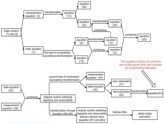
Figure 1.
The entire estimation method.
5. Numerical Simulation
Considering a linear discrete-time singular system in the form of Equations (1) and (2), we set:
The initial values of the system are and The estimation initial values of the system are and . This numerical example represents a non-causal system and the matrix transformation process can be found in the Appendix A.
Figure 2, Figure 3, Figure 4, Figure 5, Figure 6 and Figure 7 show the proposed filtering results for six sub-states with 100 steps. Figure 8 show the root mean square error (RMSE) results using 1000 steps. From Figure 2, Figure 3, Figure 4, Figure 5, Figure 6 and Figure 7, we can see that each component of state estimation can effectively follow the true state component. From Figure 8, we can see that each component of state estimation tends to converge.
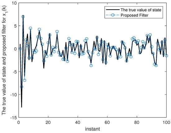
Figure 2.
The true value of state and proposed filter for .
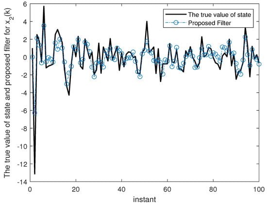
Figure 3.
The true value of state and proposed filter for .
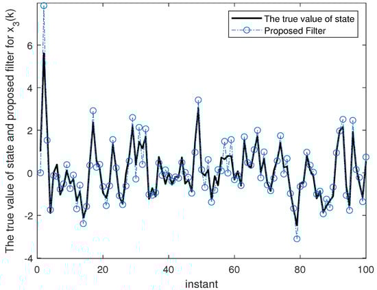
Figure 4.
The true value of state and proposed filter for .
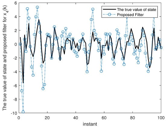
Figure 5.
The true value of state and proposed filter for .
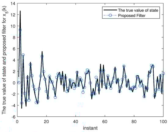
Figure 6.
The true value of state and proposed filter for .
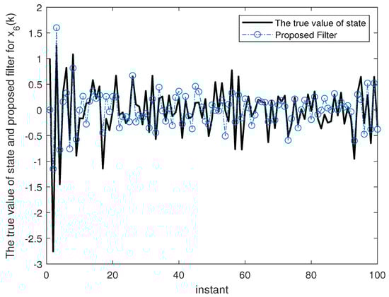
Figure 7.
The true value of state and proposed filter for .
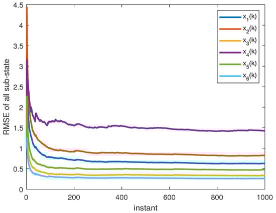
Figure 8.
The RMSE of all sub-state.
6. Conclusions and Future Work
This paper considers the causality of the system and proposes a state estimation method based on the Kalman filter for linear discrete-time rectangular singular systems. The feasibility of the algorithm is verified through numerical simulation. Compared to existing methods, the main contribution of this paper is to propose a state estimation method for linear rectangular singular systems which is non-causal, providing a new approach for solving the state estimation problem of rectangular singular systems. Although the numerical simulations in this paper have shown that the proposed filter tends to converge, this paper has not yet conducted a theoretical analysis of the convergence and stability. Compared to general systems, theoretical analysis of convergence and stability about rectangular singular systems could be more difficult and more complex due to the less constrained information in the state equation, which needs to be studied in the future. In addition, non-causal properties may also exist in nonlinear singular systems. For example, at a certain moment, the matrix pair of the nonlinear singular system, which can be obtained by Taylor expansion, may be non-causal. Therefore, more research is needed to solve nonlinear singular systems with non-causal properties. Furthermore, the control problem of rectangular singular systems is also worth studying. For example, if the system (1) has some input as on the right-hand side, how to gain the state estimation and how to solve the control problems? These problems also need to be solved.
Author Contributions
Conceptualization, J.Z., C.W. and W.L.; methodology, C.W.; software, J.Z.; validation, J.Z.; formal analysis, J.Z.; investigation, J.Z.; resources, J.Z.; data curation, J.Z.; writing—original draft preparation, J.Z.; writing—review and editing, C.W. and W.L.; visualization, C.W.; supervision, C.W. and W.L.; project administration, C.W.; funding acquisition, W.L. All authors have read and agreed to the published version of the manuscript.
Funding
This research was funded by The National Natural Science Foundation of China 62125307, 61933013 and U22A2046.
Institutional Review Board Statement
Not applicable.
Informed Consent Statement
Not applicable.
Data Availability Statement
Data are contained within the article.
Conflicts of Interest
The authors declare no conflict of interest.
Appendix A. The Matrix Transformation of the Numberical Simulation
The transformation process of the matrix E and A can be Summarized in two steps. The first step: Using the first type of restricted equivalence transformation(RET).
The second step: transformation through Equations (36)–(60):
The transformation process of the matrix H is Related to matrix E, and matrix H is transformed to:
According to the transformation in this section, the system in “Numerical Simulation” is non-causal system. The 2nd row and 3rd row of the measurement equation are selected to add into the state equation.
References
- Hanieh, M.; Yao, H. Extended Kalman filtering for state estimation of a Hill muscle model. IET Control Theory Appl. 2018, 12, 384–394. [Google Scholar]
- Li, Z.; Sun, M.; Duan, Q.; Mao, Y. Robust State Estimation for Uncertain Discrete Linear Systems with Delayed Measurements. Mathematics 2022, 10, 1365. [Google Scholar] [CrossRef]
- Mahdieh, A.; Majid, H. Distributed trust-based unscented Kalman filter for non-linear state estimation under cyber-attacks: The application of manoeuvring target tracking over wireless sensor networks. IET Control Theory Appl. 2021, 15, 1987–1998. [Google Scholar]
- Wang, M.; Liu, W.F.; Wen, C. A High-Order Kalman Filter Method for Fusion Estimation of Motion Trajectories of Multi-Robot Formation. Sensors 2022, 22, 5590. [Google Scholar] [CrossRef] [PubMed]
- Zhang, Q.; Xu, Y.; Wang, X.; Yu, Z.; Deng, T. Real-Time Wind Field Estimation and Pitot Tube Calibration Using an Extended Kalman Filter. Mathematics 2021, 9, 646. [Google Scholar] [CrossRef]
- Kalman, R.E. A new approach to linear filtering and prediction problems. J. Basic Eng. 1960, 82, 35–45. [Google Scholar] [CrossRef]
- Huang, Y.; Xue, C.; Zhu, F.; Wang, W.; Zhang, Y.; Chambers, J.A. Adaptive Recursive Decentralized Cooperative Localization for Multirobot Systems with Time-Varying Measurement Accuracy. IEEE Trans. Instrum. Meas. 2021, 70, 1–25. [Google Scholar] [CrossRef]
- Wang, J.; Wen, C. Real-Time Updating High-Order Extended Kalman Filtering Method Based on Fixed-Step Life Prediction for Vehicle Lithium-Ion Batteries. Sensors 2022, 22, 2574. [Google Scholar] [CrossRef]
- Huang, Y.; Zhang, Y.; Wu, Z.; Li, N.; Chambers, J. A Novel Adaptive Kalman Filter with Inaccurate Process and Measurement Noise Covariance Matrices. IEEE Trans. Autom. Control 2018, 63, 594–601. [Google Scholar] [CrossRef]
- Lu, Z.; Wang, N.; Dong, S. Improved Square-Root Cubature Kalman Filtering Algorithm for Nonlinear Systems with Dual Unknown Inputs. Mathematics 2024, 12, 99. [Google Scholar] [CrossRef]
- Rosenbrock, H.H. Structural properties of linear dynamical systems. Int. J. Control 1974, 20, 191–202. [Google Scholar] [CrossRef]
- Dai, L. Singular Control Systems; Springer: Berlin/Heidelberg, Germany, 1989. [Google Scholar]
- Lewis, F.L.; Mertzios, V.G. Recent advances in singular systems. Circuits Syst. Sign. Process. 1989, 8, 341–355. [Google Scholar]
- Feng, Y.; Yagoubi, M.; Chevrel, P. Dilated LMI characterisations for linear time-invariant singular systems. Int. J. Control 2010, 11, 2276–2284. [Google Scholar] [CrossRef]
- Xia, Y.Q.; Boukas, E.K.; Shi, P.; Zhang, J.H. Stability and stabilization of continuous-time singular hybrid systems. Automatica 2009, 45, 1504–1509. [Google Scholar] [CrossRef]
- Jin, Z.; Zhang, Q.; Zhang, Y. The Impulse Analysis of the Regular Singular System via Kronecker Indices. Int. Conf. Appl. Math. Model. Stat. Appl. 2018, 143, 62–67. [Google Scholar]
- Zheng, J.; Ran, C. Robust time-varying Kalman predictor for uncertain singular system with missing measurement and colored noises. In Proceedings of the 2022 34th Chinese Control and Decision Conference (CCDC), Hefei, China, 15–17 August 2022; Volume 34, pp. 3483–3488. [Google Scholar]
- Nosrati, K.; Belikov, J.; Tepljakov, A.; Petlenkov, E. Extended fractional singular Kalman filter. Appl. Math. Comput. 2023, 448, 127950. [Google Scholar] [CrossRef]
- Nosrati, K.; Shafiee, M. Kalman filtering for discrete-time linear fractional-order singular systems. IET Control Theory Appl. 2018, 12, 1254–1266. [Google Scholar] [CrossRef]
- Lu, X.; Wang, L.; Wang, H.; Wang, X. Kalman Filtering for Delayed Singular Systems with Multiplicative Noise. IEEE/CAA J. Autom. Sin. 2016, 3, 51–58. [Google Scholar]
- Yu, X.; Pu, S.; Li, J. An Optimal Filter for Singular Systems with Stochastic Multiplicative Disturbance. IEEE Trans. Circuits Syst. Express Briefs 1989, 67, 3607–3611. [Google Scholar] [CrossRef]
- Zhang, H.; Xie, L.; Soh, Y.C. Optimal Recursive Filtering, Prediction, and Smoothing for Singular Stochastic Discrete-Time Systems. IEEE Trans. Autom. Control 1999, 44, 2154–2158. [Google Scholar] [CrossRef]
- Zhang, Q.H.; Lu, J.G. Positive real lemmas for singular fractional order systems. IET Control Theory Appl. 2020, 14, 2805–2813. [Google Scholar] [CrossRef]
- Wang, J.X.; Wu, H.-C.; Ji, X.-F.; Liu, X.H. Robust Finite-Time Stabilization for Uncertain Discrete-Time Linear Singular Systems. IEEE Access 2020, 8, 100645–100651. [Google Scholar] [CrossRef]
- Cui, Y.; Shen, J.; Feng, Z.; Chen, Y. Stability Analysis for Positive Singular Systems with Time-Varying Delays. IEEE Trans. Autom. Control 2018, 63, 1487–1494. [Google Scholar] [CrossRef]
- Liu, H.X.; Lin, C.; Cheng, B.; Ge, W.T. Stabilization for Rectangular Descriptor Fractional Order Systems. IEEE Access 2019, 7, 177556–177561. [Google Scholar] [CrossRef]
- Abhinav, K.; Mamoni, P.M.K. Impulse Eliminations for Rectangular Descriptor Systems: A Unified Approach. IEEE Control Syst. Lett. 2023, 7, 1357–1362. [Google Scholar]
- Xu, S.-Y.; James, L. Robust Control and Filtering of Singular Systems; Springer: Berlin/Heidelberg, Germany, 2006; p. 332. [Google Scholar]
- Zhang, G.S. Regularizability, controllability and observability of rectangular descriptor systems by dynamic compensation. In Proceedings of the 2006 American Control Conference, Minneapolis, MN, USA, 14–16 June 2006; pp. 4393–4398. [Google Scholar]
- Tian, H.-W.; Shi, Y. Reduced-order Kalman recursive filter for non-square descriptor systems with correlated noise. In Proceedings of the 30th Chinese Control Conference, Yantai, China, 22–24 July 2011; pp. 1428–1431. [Google Scholar]
- Wen, C.-B.; Cheng, X.S. A State Space Decomposition Filtering Method for a Class of Discrete-Time Singular Systems. IEEE Access 2019, 7, 50372–50379. [Google Scholar] [CrossRef]
- Duan, G.R.; Chen, Y. Generalized regularity and regularizability of rectangular descriptor systems. J. Control Theory Appl. 2007, 5, 159–163. [Google Scholar] [CrossRef]
Disclaimer/Publisher’s Note: The statements, opinions and data contained in all publications are solely those of the individual author(s) and contributor(s) and not of MDPI and/or the editor(s). MDPI and/or the editor(s) disclaim responsibility for any injury to people or property resulting from any ideas, methods, instructions or products referred to in the content. |
© 2023 by the authors. Licensee MDPI, Basel, Switzerland. This article is an open access article distributed under the terms and conditions of the Creative Commons Attribution (CC BY) license (https://creativecommons.org/licenses/by/4.0/).