Article

Adaptive Trajectory Tracking Algorithm for the Aerospace Vehicle Based on Improved T-MPSP

1
School of Aerospace Engineering, Huazhong University of Science and Technology, Wuhan 430074, China
2
Aerospace Technology Institute of China Aerodynamics Research and Development Center, Mianyang 621000, China
*
Author to whom correspondence should be addressed.
Mathematics 2023, 11(9), 2160; https://doi.org/10.3390/math11092160
Submission received: 18 January 2023 / Revised: 25 April 2023 / Accepted: 2 May 2023 / Published: 4 May 2023

Abstract

:
To deal with the uncertainty and disturbance that exist in the tracking system of an aerospace vehicle, an adaptive trajectory-tracking method based on a novel tracking model predictive static programming (T-MPSP) is proposed. Firstly, to make the proposed method more adaptive to uncertain parameter deviations, an extended Kalman filter (EKF) parameter correction strategy is designed. Then, the control constraints are considered to form a novel T-MPSP algorithm. By combining the parameter correction strategy with the improved T-MPSP algorithm, a novel adaptive tracking guidance scheme is presented. Finally, simulations are carried out to demonstrate the effectiveness of the proposed method.

1. Introduction

For the past few decades, aerospace vehicles have been applied in both military and civilian fields, and their performance has been very compelling. For missions involving aerospace vehicles, a good trajectory-tracking ability is the essential prerequisite for the successful application of the vehicles [1]. In a traditional trajectory-tracking process for an aerospace vehicle, the dynamic model of the vehicle and the desired trajectory satisfying all the constraints are given in advance. Then, the control methods are designed to guide the vehicle to track the desired trajectory. However, the trajectories of aerospace vehicles usually cover a wide range of altitudes, which may lead to a dramatic change in the atmospheric environment during the trajectory-tracking process. In addition to the disturbance brought about by the dramatic change in the external environment, there are also uncertainties about the dynamic system of the vehicles [2,3]. Thus, the precise model information is not always available, and the traditional trajectory-tracking method cannot achieve satisfactory performance under these circumstances. As a result, the design of the novel trajectory-tracking control method to cope with disturbance and uncertainty is very important.
One of the most commonly used control architectures for trajectory-tracking control is the proportional-integral-derivative (PID) controller and its variants [4,5,6,7], which are known for the simplicity of their framework. To improve the tracking performance, many modern control theories, including intelligent optimization [4], feedback control [5], and fuzzy control [6,7], have been applied to the trajectory-tracking method design process. Another popular control architecture for trajectory-tracking control derives from the sliding mode control theory. In [8], the sliding mode control theory is applied to make the tracking error converge to zero in a finite time period. As an improvement of the method in [8], the fixed-time control theory was combined with the sliding mode control theory. The robustness of the resulting tracking laws was further enhanced [9,10]. Recently, the neural network and adaptive updating laws were applied to the sliding mode control framework. The convergence of the tracking error was ensured by the sliding mode control approach, and any system uncertainties were handled by the neural network [11].
In addition, the nonlinear model predictive control (NMPC) was applied to the trajectory-tracking control [12,13,14,15]. However, several issues exist in the implementation of the NMPC-based tracking methods, which are summarized as follows: (1) a universal and exact model of the whole tracking system is difficult to acquire, (2) the calculation speed of the NMPC cannot meet the requirement in practice. A feasible way to cope with these issues is to use model predictive static programming (MPSP) [16], which combines the characteristics of approximate dynamic programming [17] and NMPC. The MPSP has been proven to be an effective method to cope with two-point boundary value problems with terminal constraints, which has significant advantages: (1) the terminal constraints are transformed into linear equality constraints with only the control variable to be optimized, (2) the closed analytical expression of the appropriate objective function is acquired from the static algorithm, (3) the sensitivity matrix of the algorithm can be calculated skillfully using recursion, which improves the calculation speed. The MPSP method has been used in many applications, such as in the trajectory control of launch vehicles, reentry guidance, cooperative control, etc. [18,19,20]. Typically, the MPSP method aims to improve the terminal accuracy by iteratively discretizing and updating. For a trajectory-tracking problem, only the terminal-tracking accuracy can be guaranteed using the MPSP method, and its computing time increases exponentially with the number of discrete nodes that are tracked. To deal with this drawback, the T-MPSP is put forward to track a trajectory over a receding horizon window. Meanwhile, the predicted time horizon can be set manually to balance the computational efficiency and the precision, which is another advantage of the T-MPSP algorithm [21,22].
Some trajectory-tracking methods are based directly on the input and output data of the system. For example, a robust model-free controller for trajectory-tracking control is proposed in Ref. [23]. No dynamic model information of the controlled system is needed, and the resulting controller is a combination of the PID controller and the sliding mode control. As an improvement of the work in Ref. [23], a forecasting-based data-driven model-free adaptive sliding mode attitude control method is proposed for the post-capture combined spacecraft with unknown inertial properties and external disturbances [24]. To cope with the unknown dynamics of the system, a model-free control method is proposed via the time-varying compensation of the un-modeled system [25]. An iterative sliding mode control technique is utilized to design the adaptive model-free trajectory-tracking method in Ref. [26]. Although these model-free control methods can deal with model uncertainties, the operation data require a huge memory size, and the computing burden is heavy.
Hence, considering the uncertainty and disturbance that exist in the tracking system of the aerospace vehicle, an adaptive trajectory-tracking method based on the novel T-MPSP is proposed. Firstly, to cope with the uncertain parameter deviations, an EKF parameter correction strategy is designed. Then, the control constraints are considered to form a novel T-MPSP algorithm. By combining the parameter correction strategy with the improved T-MPSP algorithm, an adaptive tracking guidance scheme is presented. Finally, simulations are carried out under various deviation conditions to verify the reliability and robustness of the proposed method.
The main contributions of this paper are summarized as follows:
(1)
To our best knowledge, no existing methods have applied the EKF with the T-MPSP to solve the trajectory problems of aerospace vehicles.
(2)
Compared with the MPSP method in [18,19,20], the proposed method has a fast computing speed and high accuracy.
(3)
Compared with [21,22,23], the proposed scheme can cope with the control constraints.
The rest of this paper is organized as follows: Section 2 presents the model of the aerospace vehicle. Section 3 presents the online parameter identification method and the improved T-MPSP algorithm. The simulations are presented in Section 4. Finally, the conclusion is presented in Section 5.

2. Model of the Aerospace Vehicle

In this section, first, the dynamic model describing the motion of the aerospace vehicle is presented. Then, the constraints that should be satisfied are introduced.

2.1. Dynamic Equations

The three-dimensional mass point dynamic equations [22,27] of the aircraft in the longitudinal plane are
d h d t = v sin γ d v d t = T cos α D m g sin γ d γ d t = T sin α + L m v g v cos γ + v r cos γ d m d t = T g 0 I sp
where h , v , γ , α and m represent the altitude, velocity, flight path angle, angle of attack (AOA), and mass, respectively. g and g 0 represent the gravitational acceleration at the current altitude and on the earth’s surface, respectively. I s p represents the specific impulse of the engine. T, L and D denote the engine thrust, aerodynamic lift, and drag, respectively, which are defined as
T = 0.029 ϕ I s p ρ g 0 v C T A C L = 1 2 ρ v 2 S ref C L ( Ma , α ) D = 1 2 ρ v 2 S ref C D ( Ma , α )
where C T , C L , and C D denote the thrust, lift and drag coefficients, respectively. ϕ denotes the throttle. ρ , S ref and Ma denote the atmospheric density, reference area, and Mach number, respectively.

2.2. Flight Constraints

To ensure flight safety, the dynamic pressure constraint is considered, which is defined as
q = 1 2 ρ v 2 q max
In addition, the aircraft must satisfy the terminal constraints, which are described as
h f h f * ε h v f v f * ε v γ f γ f * ε γ
where the subscript f refers to the final value and the superscript * refers to the desired value. ε h , ε v , and ε γ represent the deviation thresholds of the terminal altitude, velocity, and flight path angle, respectively.
The control variables considered are α and the throttle ϕ , the constraints of which are as follows:
α min α α max ϕ min ϕ ϕ max
Additionally, to prevent the control variable from changing too drastically, the rate of AOA must satisfy the following constraint:
α ˙ min α ˙ α ˙ max

3. The Trajectory-Tracking Strategy

In this section, we will introduce an online parameter identification method and an improved T-MPSP algorithm. By combining these two methods, an adaptive trajectory-tracking guidance algorithm based on an improved T-MPSP will be presented.

3.1. Online Parameter Identification Method

Since an accurate model can improve the trajectory-tracking accuracy, a parameter correction strategy based on the EKF is designed in this subsection. In the actual tracking process, there are deviations in the parameters of atmospheric density, thrust coefficient, lift coefficient, and drag coefficient, which will make the model inaccurate. We define these parameters as
ρ = ρ * 1 + Δ ρ , C T = C T * 1 + Δ C T , C L = C L * 1 + Δ C L , C D = C D * 1 + Δ C D
where ρ * , C T * , C L * and C D * are the desired values. ρ , C T , C L and C D are the actual values. Δ ρ , Δ C T , Δ C L , and Δ C D respectively represent the unknown deviation of each parameter. These unknown deviations are written in an overall form as
β = Δ ρ Δ C T Δ C L Δ C D T
Defining x = h v γ m , the following dynamic equations are obtained from (1) and (7) as
x ˙ = f x , u , β
in which
f x , u , β = v sin γ T * 1 + Δ ρ 1 + Δ C T cos α D * 1 + Δ ρ 1 + Δ C D m g sin γ T * 1 + Δ ρ 1 + Δ C T sin α + L * 1 + Δ ρ 1 + Δ C L m v g v cos γ + v r cos γ T * 1 + Δ ρ 1 + Δ C T g 0 I s p
Since the EKF algorithm [28] needs to augment the unknown parameters into the state variables of the system, the new augmented dynamic equation is defined as
x ˙ a = f a x a , u + ω a = f x , u , β 0 + ω a
where
x a = h v γ m Δ ρ Δ C T Δ C L Δ C D T u = α ϕ T
ω a represents the uncorrelated zero-mean white Gaussian noise. To identify the unknown parameters, the EKF algorithm also requires the measurement information of the unknown parameters. The measurement equation is expressed as
y = x m a x m a z m q m = h x a , u + v a = x ρ v 2 2 m C x + T m ρ v 2 2 m C z ρ v 2 2 + v a
where x m , a x m , a z m and q m denote the state values, axial acceleration, normal acceleration and dynamic pressure measured by the sensor, respectively. v a represents the uncorrelated zero-mean Gaussian white noise. C x and C z refer to axial and normal force coefficients, respectively. The calculation formulas of C x and C z are
C x = C L sin α C D cos α C z = C L cos α C D sin α
Then, the two-step online parameter identification method will be introduced as follows:
  • Prediction
First, the prior estimate of the state at the current time instant k is
x ^ a k = x ^ a k 1 + f x ^ a k 1 Δ t + F k f x ^ a k 1 2 Δ t 2
where F k represents the Jacobian matrix of the augmented state equation f a x ^ a k 1 to estimate the state x ^ a k 1 at the previous time instant and Δ t represents the sampling time interval. Then, the error covariance matrix of the current time instant k according to the equation is acquired as
P k = Φ k P k 1 Φ k T + Q k
where Φ k = I + F k Δ t represents the state transition matrix, and Q k represents the noise covariance matrix.
b.
Update
Using the error covariance matrix P k , we update the Kalman filter gain coefficient K k at the current time instant k as
K k = P k H k T H k P k H k T + V k 1
where V k represents the measurement noise covariance matrix, and H k represents the Jacobian matrix of the prior estimate x ^ a k of the state from the measurement equation y x ^ a k . Subsequently, the error covariance matrix is updated as
P k = I K k H k P k I K k H k T + K k R k K k T
The measurement correction is updated as
Δ y k = y k y x ^ a k
where y k represents the actual measurement value.
Finally, we update the posterior estimate of the state at the current time instant k using
x ^ a k = x ^ a k + K k Δ y k
x ^ a k of the augmented state has been obtained through the EKF algorithm, from which the estimated value of the corresponding unknown parameter β is also obtained. Thus, the new model that accounts for uncertain derivations is obtained by substituting the estimated value of β into (10).
Remark 1.
An imprecise model will make it difficult for the trajectory-tracking method design, and uncertain parameter deviations will affect the accuracy of the model. Hence, a parameter correction strategy based on the EKF is designed in this subsection. By applying the EKF algorithm, the augmented state x ^ a k is obtained, from which the estimated value of the corresponding unknown parameter β is also obtained. Then, the exact model that considers uncertain derivations is obtained.

3.2. Improved T-MPSP Algorithm

According to (1), the state variables are X = h , v , γ , m T , the control variables are U = α , ϕ T , and the output variables are Y = h , v , γ T . The discrete form of the state equation and output equation of a continuous nonlinear system is expressed as
X k + 1 i = F k X k i , U k i
Y k i = h X k i
where X n , U m and Y p denote the state, control, and output variables, respectively. k = 1 , 2 , , N y represents the k th sampling point, and N y represents the total length of the prediction time domain. k = 1 and k = N y represent the starting and ending points of the prediction time domain, respectively, and i represents the number of iterations.
The main objective of the trajectory-tracking algorithm is to find the suitable control variables U k i + 1 to make the output Y k i + 1 as close to the desired output Y k * ( k = 2 , 3 , , N y ) as possible at each sampling time; that is, Y k i + 1 Y k * , where U k i represents the control variables at the current i th iteration, and U k i + 1 represents the control variables for the next iteration.
Similarly, Y k i is the current output, and Y k i + 1 is the output of the next iteration. We should also add a performance index that minimizes the deviation of the control variables to avoid overly drastic changes in the control variables. Therefore, the following objective function is proposed:
J = 1 2 k = 2 N y Y k i + 1 Y k * T Q k i Y k i + 1 Y k * + 1 2 k = 1 N y 1 U k i + 1 U k i T R k i U k i + 1 U k i
where Q k i and R k i are both the positive definite weight matrix at the i th iteration.
The deviation vectors between two consecutive iterations at the same time are defined as follows:
Y k i + 1 = Y k i + Δ Y k i
X k i + 1 = X k i + Δ X k i
U k i + 1 = U k i + Δ U k i
By expanding the Taylor series of Δ Y k i and ignoring its higher-order terms, we obtain
Δ Y k i d Y k i = Y k X k d X k i
Similarly, we obtain
Δ X k + 1 i d X k + 1 i = F k X k d X k i + F k U k d U k i
where d X k i and d U k i represent deviations in the state variables and control variables at the k th time instant, respectively. By substituting (27) into (26), we obtain
d Y k i = Y k X k F k 1 X k 1 d X k 1 i + Y k X k F k 1 U k 1 d U k 1 i
where d X k 1 is also expanded into an equation composed of d X k 2 and d U k 2 , and the corresponding equation is substituted into (29). By successively substituting d X k , d X k 1 , d X 2 into the expression of d Y k i , we obtain
d Y k i = A k i d X 1 i + B 1 k i d U 1 i + B 2 k i d U 2 i + + B k 1 k i d U k 1 i
It is obvious that d X 1 i = 0 . Then, (30) is simplified to
d Y k i = j = 1 k 1 B j k i d U j i
B j k i = Y k X k F k 1 X k 1 F j + 1 X j + 1 F j U j   , k = 2 , 3 , , N y
where B j k i is called the sensitivity matrix. Then, the deviations in the output variables and control variables at each sampling time are formed into a linear equation, in which each d U j i is a variable to be optimized. (32) is calculated recursively in the following way:
A k k i = I n × n A j k i = A j + 1 k i F j X j B j k i = Y k X k A j + 1 k i F j U j
where k = 2 , 3 , , N y , j = k 1 , k 2 , , 1 , when j k , B j k i = 0 p × m .
According to (24) and (26), and considering the small approximation Δ Y k i d Y k i , Δ U k i d U k i , we obtain
Y k i + 1 Y k * = Δ Y k i + Y k i Y k * = Δ Y k i Δ Y k * i = d Y k i Δ Y k * i U k i + 1 U k i = Δ U k i = d U k i
Hence, the objective function in (23) is rewritten as
J = 1 2 k = 2 N y d Y k i Δ Y k * i T Q k i d Y k i Δ Y k * i + 1 2 k = 1 N y 1 d U k i T R k i d U k i
In the traditional T-MPSP algorithm, the increment of the control variables is added to the performance index to indirectly constrain the control variables. However, this method cannot strictly constrain the control variables, which may fail to satisfy the constraints. Therefore, we propose an improved T-MPSP algorithm by adding control variable constraints.
The control variable constraints (5) and (6) are expressed as
U min U k i + 1 U max U ˙ min U ˙ k i + 1 = U k + 1 i + 1 U k i + 1 h U ˙ max
where h represents the sampling step size, U m . According to (34), we obtain
U min U k i + d U k i U max d U k i U max U k i d U k i U k i U min
which is simplified to
d U k i U max U k i = C 1 k i d U k i U k i U min = C 2 k i
The control magnitude constraint is thus transformed into a linear inequality constraint with the only unknown d U k i . Then, U ˙ k i + 1 is converted into
U ˙ k i + 1 = U k + 1 i + 1 U k i + 1 h = U k + 1 i + d U k + 1 i U k i + d U k i h
Thereby,
U ˙ min U k + 1 i + d U k + 1 i U k i + d U k i h U ˙ max d U k i + d U k + 1 i h U ˙ max U k + 1 i + U k i d U k i d U k + 1 i h U ˙ min + U k + 1 i U k i
which is simplified to
I m I m d U k i d U k + 1 i h U ˙ max U k + 1 i + U k i = C 3 k i I m I m d U k i d U k + 1 i h U ˙ min + U k + 1 i U k i = C 4 k i
where I m is an identity matrix of order m × m . In this way, the change rate constraint is transformed into linear inequality constraints with unknowns d U k i and d U k + 1 i . In order to facilitate the subsequent solution, (41) is rewritten in the following form:
P d U i = C 3 i P d U i = C 4 i
where P = I m I m 0 0 0 I m I m 0 0 0 0 0 0 0 I m I m , d U i = d U 1 i d U 2 i d U N 2 i d U N 1 i , C 3 i = C 3 1 i C 3 2 i C 3 N 2 i C 3 N 1 i , C 4 i = C 4 1 i C 4 2 i C 4 N 2 i C 4 N 1 i .
Therefore, combining (35) with the inequality constraints in (38) and (42) yields
min J = 1 2 k = 2 N y d Y k i Δ Y k * i T Q k i d Y k i Δ Y k * i + 1 2 k = 1 N y 1 d U k i T R k i d U k i s . t . d U k i C 1 k i d U k i C 2 k i ,   P d U i = C 3 i P d U i = C 4 i
In this paper, the Lagrangian multiplier method and the penalty function are applied to solve the NLP problem; thus, we have
L = 1 2 k = 2 N y j = 1 k 1 B j k d U j Δ Y k * T Q k j = 1 k 1 B j k d U j Δ Y k * + 1 2 k = 1 N y 1 d U k T R k d U k + 1 2 k = 1 N y 1 d U k C 1 k T σ 1 k d U k C 1 k + 1 2 k = 1 N y 1 d U k C 2 k T σ 2 k d U k C 2 k + 1 2 k = 1 N y 2 j = 1 N y 1 P k j d U j C 3 k T σ 3 k j = 1 N y 1 P k j d U j C 3 k + 1 2 k = 1 N y 2 j = 1 N y 1 P k j d U j C 4 k T σ 4 k j = 1 N y 1 P k j d U j C 4 k
where P k j represents the element of the k th row and the j th column of the matrix P . The data in the following equations are all in the same iteration i , so the superscript i is omitted for the convenience of subsequent derivation. According to the necessary conditions for first-order optimality, we obtain
L d U l = 0 R l d U l + k = 2 N y B l k T Q k j = 1 k 1 B j k d U j k = 2 N y B l k T Q k Δ Y k * + σ 1 l d U l C 1 l + σ 2 l d U l + C 2 l + k = 2 N y 2 P k l T σ 3 k j = 1 N y 1 P k j d U j k = 2 N y 2 P k l T σ 3 k C 3 k + k = 2 N y 2 P k l T σ 4 k j = 1 N y 1 P k j d U j + k = 2 N y 2 P k l T σ 4 k C 4 k = 0
where σ 1 k , σ 2 k , σ 3 k and σ 4 k are all penalty factors. By changing the positions of the terms in Equation (45), we obtain
R l + σ 1 l + σ 2 l d U l + k = 2 N y B l k T Q k j = 1 k 1 B j k d U j + k = 2 N y 2 P k l T σ 3 k j = 1 N y 1 P k j d U j + σ 4 k j = 1 N y 1 P k j d U j = k = 2 N y B l k T Q k Δ Y k * + k = 2 N y 2 P k l T σ 3 k C 3 k σ 4 k C 4 k + σ 1 l C 1 l σ 2 l C 2 l
All d U l ( l = 1 , 2 , , N y 1 ) in (46) are expressed in a matrix form as
M 11 + T 1 M 1 ( N y 2 ) M 1 ( N y 1 ) M 21 M 22 + T 2 M 2 ( N 1 ) M ( N y 1 ) 1 M ( N y 1 ) ( N y 1 ) + T N y 1 d U 1 d U 2 d U N y 1 = b 1 b 2 b N y 1
where
M i j = l = j + 1 N y B i l T Q l B j l + k = 2 N y 2 P k i T σ 3 k P k j + P k i T σ 4 k P k j b i = σ 1 i C 1 i σ 2 i C 2 i + l = 2 N y B i l T Q l Δ Y l * + k = 2 N y 2 P k i T σ 3 k C 3 k σ 4 k C 4 k T i = R i + σ 1 i + σ 2 i
By solving (47), we obtain the corrections for all control variables d U = d U 1 , d U 2 , , d U N y 1 . Finally, the updated control variables are calculated as
U i + 1 = U i + d U

3.3. Overall Structure and Operating Steps

In this subsection, we combine the online parameter identification method with the improved T-MPSP algorithm to propose an adaptive trajectorytracking guidance algorithm based on an improved T-MPSP. By applying the first-order Euler method, we obtain
X k + 1 = X k + h f X , U = F k X k , U k
where h represents the sampling step size. X k = h k , v k , γ k , m k T , U k = α k , ϕ k T and Y k = h k , v k , γ k T denote the state, control, and output variables of the aircraft, respectively. f X , U represents the state differential equation of (1). The comprehensive block diagram of the proposed method is presented in Figure 1, and the operating steps of the adaptive tracking guidance algorithm based on the improved T-MPSP are as follows:
Step 1: Parameter initialization, such as initializing the prediction time domain, sampling step size, EKF parameters, etc.
Step 2: Use the EKF algorithm to identify the parameter deviation online, which is used to correct the prediction model for the T-MPSP algorithm.
Step 3: In the improved T-MPSP algorithm, use the revised model to update the control variables until they converge or the algorithm reaches the maximum number of iterations.
Step 4: Use the first control values of the prediction time-domain window of the T-MPSP algorithm as the control variables of the current time.
Step 5: Integrate the dynamic equations using fourth-order Runge-Kutta to the next time instant.
Step 6: Determine whether the terminal time is reached. If it is reached, stop the operation. Otherwise, go to step 2 and continue with the same steps.

4. Simulations

In this section, simulations are carried out to show the effectiveness of the proposed method. First, comparison simulations against the existing T-MPSP tracking method are presented. Then, several extreme combinations of parameter deviations are considered in the simulation. Finally, the Monte Carlo simulations are carried out to verify the robustness of the proposed method.
The control parameters are initialized as
N y = 7 Q k = 1.11 0 0 0 1.96 0 0 0 5000 R k = 1000 90000
And the constraints considered in this simulation are tabulated in Table 1.

4.1. Comparison Simulations

To demonstrate the effectiveness of the proposed method, both the open-loop tracking method and the MPSP tracking law presented in [22] are considered as comparison methods in this subsection. The detailed simulation results are presented in Table 2 and Figure 1.
In Figure 2, the solid lines in blue represent the tracking results of the proposed method, dash lines in blue refer to the tracking results of the open-loop control, dot lines in pink denote the tracking results of the comparison T-MPSP method, and the reference curves are presented in dash-dot form.
For the open-loop control scenario, the tracking performance is far from satisfactory. Moreover, the maximum dynamic pressure violates the constraint, which will cause damage to the vehicle. As for the comparison T-MPSP method, the terminal accuracy is acceptable, while the overall tracking performance is not so good. In the proposed method, the terminal deviations are much smaller than in the comparison law, which confirms the effectiveness and superiority of the proposed method. The optimization process of the proposed method and the T-MPSP method requires about 1.7 s on our laptop with an AMD 1.8 GHz CPU. However, it needs about 2.8 s for the MPSP tracking method.

4.2. The Monte Carlo Simulations

In this subsection, trajectory tracking is carried out under 300 sets of deviations sampled through the LHS method. Furthermore, the distribution intervals of the four uncertain conditions are as follows:
Δ ρ 0.1 , 0.1 Δ C T 0.05 , 0.05 Δ C L 0.1 , 0.1 Δ C D 0.1 , 0.1
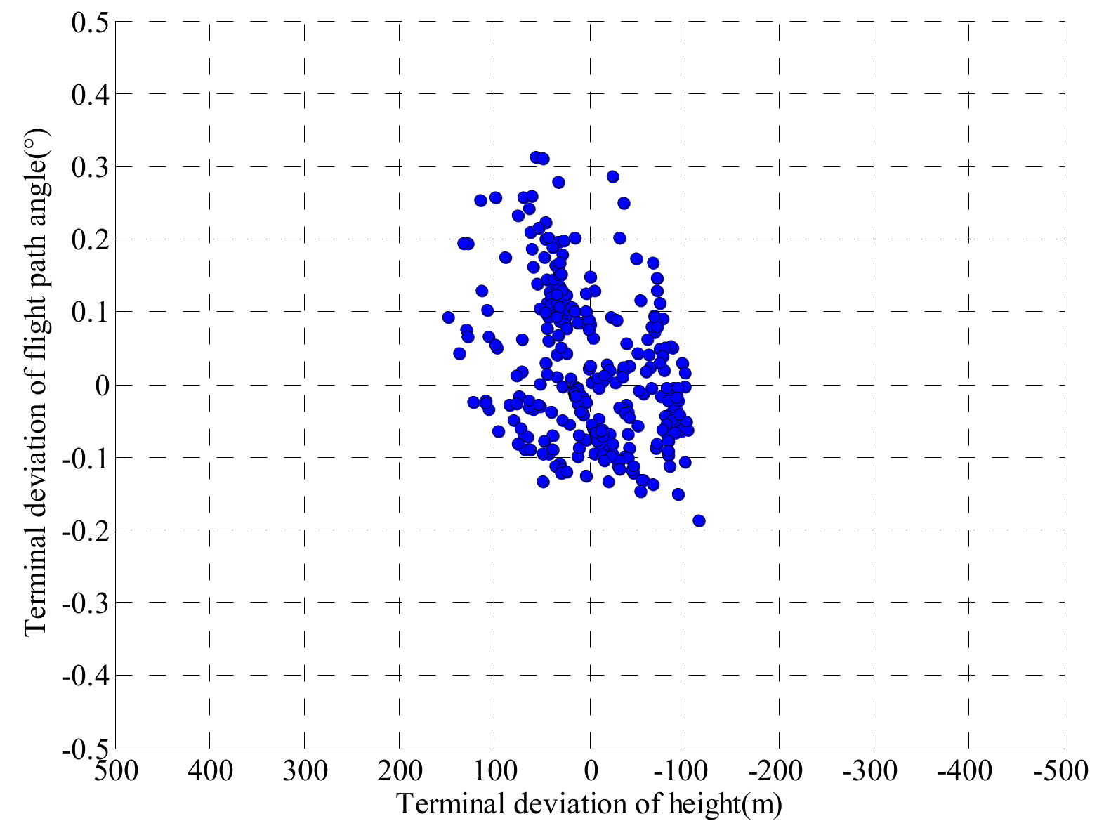
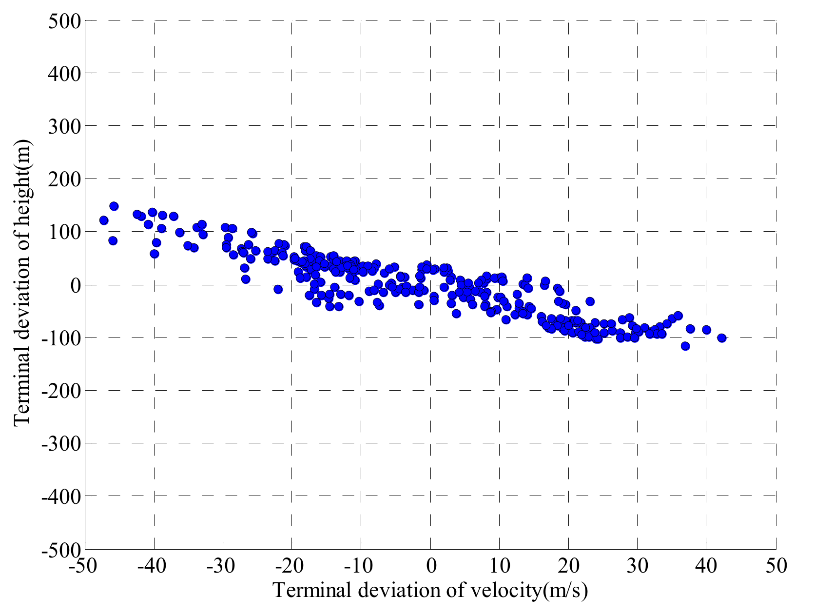
The terminal state deviations under the 300 groups of random deviations are presented in Figure 3, Figure 4 and Figure 5. The statistical maximum deviations in the terminal states are recorded in Table 3.
The maximum tracking deviation in the terminal height is less than 150 m, which is far lower than the requirements of terminal height accuracy. At the same time, the maximum tracking deviation in the terminal speed is less than 50 m/s, which also meets the requirements. In addition, the absolute value of terminal flight path angle deviation is also within the allowable range of 0.5°, and the maximum dynamic pressure also meets the constraints. These simulation results show that the novel T-MPSP method proposed in this paper has a good anti-interference ability against coefficient deviations caused by complex flight environments.

5. Conclusions

An adaptive trajectory-tracking method based on a novel tracking model predictive static programming (T-MPSP) was proposed. The proposed method had advantages in computing efficiency and tracking accuracy. Further, it was more adaptive to uncertain parameter deviations due to the parameter correction strategy. Firstly, a parameter correction strategy was designed. Then, the control constraints were considered to form a novel T-MPSP algorithm. By combining the parameter correction strategy with the improved T-MPSP algorithm, an adaptive tracking guidance scheme was presented. Finally, simulations were carried out to show the effectiveness of the proposed method. In related future research, the saturation of the input should be considered in the design of the trajectory-tracking method.

Author Contributions

Conceptualization, C.O. and Z.C.; Methodology, C.O., Z.C. and Y.L.; Investigation, Z.C. and Y.L.; Data curation, C.S.; Writing—original draft, Z C.; Supervision, Y.L. All authors have read and agreed to the published version of the manuscript.

Funding

This study was co-supported in part by the National Natural Science Foundation of China (No. 61903146).

Data Availability Statement

Not applicable.

Acknowledgments

This study has been co-supported in part by the National Natural Science Foundation of China (No. 61903146 and 61873319).

Conflicts of Interest

The authors declare no conflict of interest.

Nomenclature

Scalar
h altitude v velocity
γ flight path angle α angle of attack (AOA)
m mass g gravitational acceleration
I s p the specific impulse of the engine T the engine thrust
L the aerodynamic lift D the aerodynamic drag
C T the thrust coefficient C L the lift coefficient
C D the drag coefficient ρ the atmospheric density
ϕ the throttle S ref the reference area
Ma mach number ε the terminal deviation thresholds
ω a uncorrelated white Gaussian noise C z normal force coefficients
C x axial force coefficientskthe current time instant
Matrix
F the Jacobian matrixPthe error covariance matrix
Φ the state transition matrix Q k the noise covariance matrix
K the Kalman filter gain coefficient matrix R k the noise covariance matrix
Subscripts
maxthe maximum valueminthe minimum value
fthe final value and the superscript * the desired value
a the new augmented state

References

  1. Chai, R.; Tsourdos, A.; Savvaris, A.; Chai, S.; Chen, C. Review of advanced guidance and control algorithms for space/aerospace vehicles. Prog. Aerosp. Sci. 2021, 122, 100696. [Google Scholar] [CrossRef]
  2. Gharib, M.R.; Koochi, A.; Ghorbani, M. Path tracking control of electromechanical micro-positioner by considering control effort of the system. Proc. Inst. Mech. Eng. Part I J. Syst. Control Eng. 2021, 235, 984–991. [Google Scholar] [CrossRef]
  3. Salehi Kolahi, M.R.; Gharib, M.R.; Heydari, A. Design of a non-singular fast terminal sliding mode control for second-order nonlinear systems with compound disturbance. Proc. Inst. Mech. Eng. Part C J. Mech. Eng. Sci. 2021, 235, 7343–7352. [Google Scholar] [CrossRef]
  4. Abdalla, T.Y.; Abdulkarem, A. PSO-based optimum design of PID controller for mobile robot trajectory tracking. Int. J. Comput. Appl. 2012, 47, 30–35. [Google Scholar] [CrossRef]
  5. Madhushani, T.; Maithripala, D.S.; Berg, J.M. Feedback regularization and geometric PID control for trajectory tracking of mechanical systems: Hoop robots on an inclined plane. In Proceedings of the 2017 American Control Conference (ACC), Seattle, WA, USA, 24–26 May 2017; pp. 3938–3943. [Google Scholar]
  6. Rabah, M.; Rohan, A.; Han, Y.-J.; Kim, S.-H. Design of fuzzy-PID controller for quadcopter trajectory-tracking. Int. J. Fuzzy Log. Intell. Syst. 2018, 18, 204–213. [Google Scholar] [CrossRef]
  7. Dang, T.S.; Duong, D.T.; Le, V.C.; Banerjee, S. A combined backstepping and adaptive fuzzy PID approach for trajectory tracking of autonomous mobile robots. J. Braz. Soc. Mech. Sci. Eng. 2021, 43, 156. [Google Scholar]
  8. Shen, G.; Xia, Y.; Ma, D.; Zhang, J. Adaptive sliding-mode control for Mars entry trajectory tracking with finite-time convergence. Int. J. Robust Nonlinear Control 2019, 29, 1249–1264. [Google Scholar] [CrossRef]
  9. Ai, X.; Yu, J. Fixed-time trajectory tracking for a quadrotor with external disturbances: A flatness-based sliding mode control approach. Aerosp. Sci. Technol. 2019, 89, 58–76. [Google Scholar] [CrossRef]
  10. Sun, L.; Liu, Y. Fixed-time adaptive sliding mode trajectory tracking control of uncertain mechanical systems. Asian J. Control 2020, 22, 2080–2089. [Google Scholar] [CrossRef]
  11. Zhou, B.; Huang, B.; Su, Y.; Zheng, Y.; Zheng, S. Fixed-time neural network trajectory tracking control for underactuated surface vessels. Ocean Eng. 2021, 236, 109416. [Google Scholar] [CrossRef]
  12. Shen, C.; Shi, Y.; Buckham, B. Nonlinear model predictive control for trajectory tracking of an AUV: A distributed implementation. In Proceedings of the 2016 IEEE 55th Conference on Decision and Control (CDC), Las Vegas, NV, USA, 12–14 December 2016; pp. 5998–6003. [Google Scholar]
  13. Nascimento, T.P.; Dórea, C.E.T.; Gonçalves, L.M.G. Nonlinear model predictive control for trajectory tracking of nonholonomic mobile robots: A modified approach. Int. J. Adv. Robot. Syst. 2018, 15, 1729881418760461. [Google Scholar] [CrossRef]
  14. Chai, J.; Medagoda, E.; Kayacan, E. Adaptive and Efficient Model Predictive Control for Booster Reentry. J. Guid. Control Dyn. 2020, 43, 2372–2382. [Google Scholar] [CrossRef]
  15. Emami, S.A.; Banazadeh, A. Fault-tolerant predictive trajectory tracking of an air vehicle based on acceleration control. IET Control Theory Appl. 2019, 14, 750–762. [Google Scholar] [CrossRef]
  16. Padhi, R.; Kothari, M. Model predictive static programming: A computationally efficient technique for suboptimal control design. Int. J. Innov. Comput. Inf. Control 2009, 5, 399–411. [Google Scholar]
  17. Powell, W.B. Approximate Dynamic Programming: Solving the Curses of Dimensionality; John Wiley & Sons: Hoboken, NJ, USA, 2007; Volume 703. [Google Scholar]
  18. Halbe, O.; Raja, R.G.; Padhi, R. Robust reentry guidance of a reusable launch vehicle using model predictive static programming. J. Guid. Control Dyn. 2014, 37, 134–148. [Google Scholar] [CrossRef]
  19. Zheng, H.; Hong, H.; Tang, S. Model predictive static programming rendezvous trajectory generation of unmanned aerial vehicles. In Proceedings of the 2019 IEEE International Conference on Unmanned Systems (ICUS), Beijing, China, 17–19 October 2019; pp. 415–420. [Google Scholar]
  20. Wang, Y.; Hong, H.; Tang, S. Geometric control with model predictive static programming on SO (3). Acta Astronaut. 2019, 159, 471–479. [Google Scholar] [CrossRef]
  21. Tripathi, A.K.; Padhi, R. Autonomous landing for uavs using t-mpsp guidance and dynamic inversion autopilot. IFAC-PapersOnLine 2016, 49, 18–23. [Google Scholar] [CrossRef]
  22. Wang, M.; Zhang, S. Adaptive trajectory tracking algorithm based on tracking model-predictive-static-programming. Acta Aeronaut. Astronaut. Sin. 2018, 39, 322105–322113. [Google Scholar]
  23. Kara, T.; Mary, A. Robust trajectory tracking control of robotic manipulators based on model-free PID-SMC approach. J. Eng. Res. 2018, 6, 170–188. [Google Scholar]
  24. Emami, S.A.; Banazadeh, A. Intelligent trajectory tracking of an aircraft in the presence of internal and external disturbances. Int. J. Robust Nonlinear Control. 2019, 29, 5820–5844. [Google Scholar] [CrossRef]
  25. Dou, L.; Su, X.; Zhao, X.; Zong, Q.; He, L. Robust tracking control of quadrotor via on-policy adaptive dynamic programming. Int. J. Robust Nonlinear Control. 2021, 31, 2509–2525. [Google Scholar] [CrossRef]
  26. Qiu, X.; Hua, C.; Chen, J.; Zhang, L.; Guan, X. Model-free adaptive iterative sliding mode control for a robotic exoskeleton trajectory tracking system. Int. J. Syst. Sci. 2020, 51, 1782–1797. [Google Scholar] [CrossRef]
  27. Murillo, O.J. A Fast Ascent Trajectory Optimization Method for Hypersonic Air-Breathing Vehicles. Ph.D. Thesis, Iowa State University, Ames, IA, USA, 2010. [Google Scholar]
  28. Lopez-Sanchez, I.; Montoya-Chairez, J.; Perez-Alcocer, R.; Moreno-Valenzuela, J. Experimental Parameter Identifications of a Quadrotor by Using an Optimized Trajectory. IEEE Access 2020, 8, 167355–167370. [Google Scholar] [CrossRef]
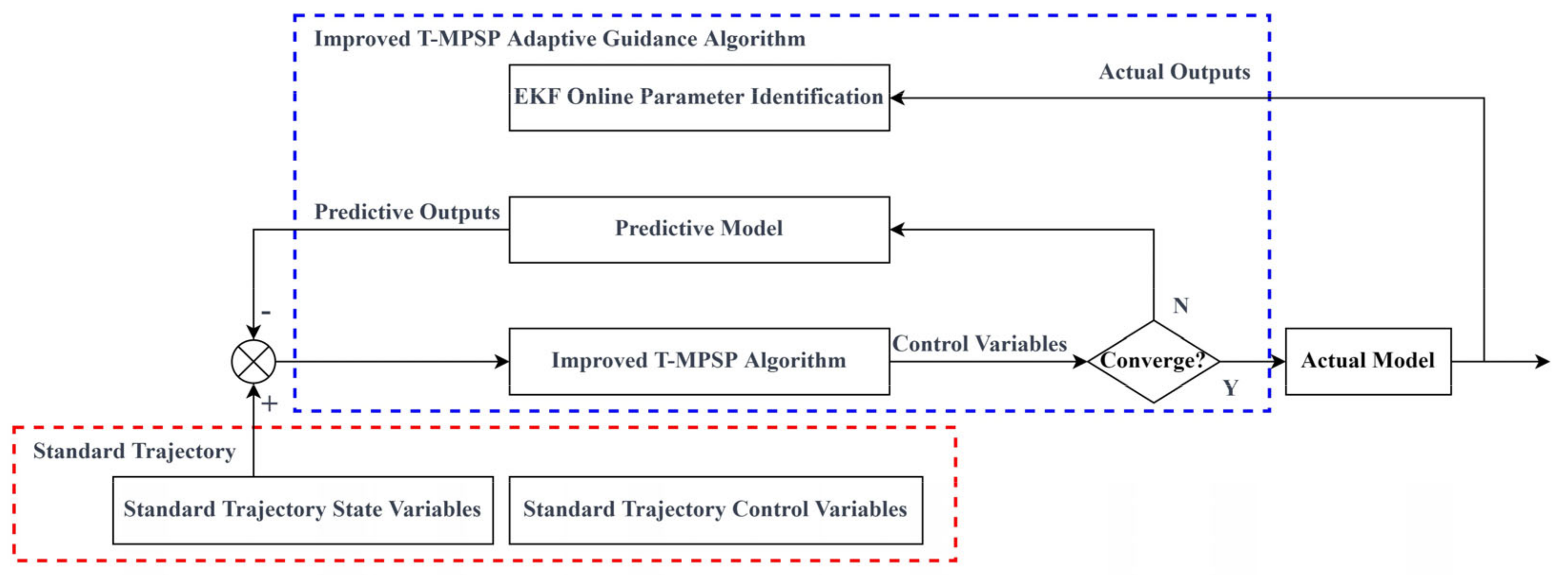
Figure 1. The block diagram of the proposed method.
Mathematics 11 02160 g001
Figure 2. Comparison results.
Mathematics 11 02160 g002
Figure 3. Terminal state deviation distributions.
Mathematics 11 02160 g003
Figure 4. Terminal state deviation distributions (left view).
Mathematics 11 02160 g004
Figure 5. Terminal state deviation distributions (vertical view).
Mathematics 11 02160 g005
Table 1. Constraints.
Process constraints q max 150 (kPa)
Control constraints [ α min , α max ] [ 3 , 21 ] (°)
[ ϕ min , ϕ max ] [ 0 , 2 ]
[ α ˙ min , α ˙ max ] [ 5 , 5 ] ( / s )
Terminal constraint ε h 500 (m)
ε v 50 (m/s)
ε γ 0.5 (°)
Table 2. Comparison results.
Terminal Height Deviations (m)Terminal Velocity Deviations (m/s)Terminal Flight Path Angle Deviations (°)
Proposed method32.95 −12.53 0.279
Open-loop tracking method−444.49 272.40 1.124
T-MPSP method−242.36 −15.48 0.025
Table 3. Maximum tracking deviations.
Terminal Height Deviations (m)Terminal Velocity Deviations (m/s)Terminal Flight Path Angle Deviations (°)Dynamic Pressure (kPa)
148.73 47.26 0.313 142.12
Disclaimer/Publisher’s Note: The statements, opinions and data contained in all publications are solely those of the individual author(s) and contributor(s) and not of MDPI and/or the editor(s). MDPI and/or the editor(s) disclaim responsibility for any injury to people or property resulting from any ideas, methods, instructions or products referred to in the content.