Abstract
In this paper, a new fixed-time convergence guidance law is proposed against maneuvering targets in the three-dimensional (3-D) engagement scenario. The fixed-time stability theory is used to zero the line-of-sight (LOS) angle rate, which will ensure the collision course and the impact of the target. It is proven that the convergence of the LOS angle rate can be achieved before the final impact time of the guidance process, regardless of the initial conditions. Furthermore, the convergence rate is merely related to control parameters. In theoretical analysis, the convergence rate and upper bound are compared with that of other laws to show the potential advantages of the proposed guidance law. Finally, simulations are carried out to illustrate the effectiveness and robustness of the proposed guidance law.
Keywords:
three-dimensional engagement; maneuvering target; LOS angle rate; collision course; fixed-time convergence MSC:
70E60; 93B12; 93C35; 93C85; 34A34
1. Introduction
During a typical missile guidance process, the most important stage is the terminal guidance phase, which plays a decisive role in determining the missile’s intercept performance [1]. In the terminal guidance phase, the target may be maneuvering. On the other hand, the time left for impacting the target is usually very short. Therefore, novel guidance laws with a fast convergence rate to ensure the impact and robustness to target maneuvers have great significance for the missile’s performance.
In order to improve the missile’s performance, many modern theories are utilized to design guidance laws. An effective way to improve the robustness of guidance laws is to apply the control theory. In [2], the guidance law was derived from solving the associated Hamilton–Jacobi function. In [3], based on the nonlinear robust filtering method to estimate the LOS rate, a guidance law was proposed considering input saturation as well as system stability. Although strong robustness was obtained and exhibited, the guidance laws cannot achieve finite-time convergence.
Another approach is to apply the Lyapunov asymptotic stability theory. In [4], a quadratic Lyapunov candidate function was proposed. By a particular selection of LOS angle function, the resulting guidance law can be free of singularities. In [5], a Lyapunov candidate function concerning the heading angle error was proposed, and the exact expression of the flight time was derived. The incomplete beta function was used, and the flight time can be adjusted by a single control parameter. As an improvement of the work in [5], another Lyapunov-based guidance strategy was proposed in [6] with impact angle constraints. In [7], the impact time constraint was considered, and the resulting guidance law can zero the heading error angle to ensure the collision course. In [8], a novel adaptive integrated guidance and control law was designed with a barrier Lyapunov function; the resulting guidance law can handle input saturation and constraints of angles. This group of guidance laws was based on the Lyapunov asymptotic stable theory, and only guaranteed the convergence of the system as time approached infinitely. Moreover, the targets were assumed stationary in the design of the guidance law. Obviously, they are theoretically imperfect.
As an improvement of asymptotic convergence law, guidance laws that can ensure finite-time convergence were investigated. A guidance law based on finite-time convergence theory was proposed in [9], which was an early work considering both finite-time convergence and target maneuver together. The LOS rate converged to zero or a small neighborhood of zero in finite time under the proposed guidance law. Then, the work in [9] was improved by taking the autopilot dynamic into account [10,11]. In [12], based on sliding mode control theory, a finite-time convergence guidance law with impact angle constraint was proposed, and the guidance command was generated to enforce terminal sliding mode on the designed switching surface from nonlinear engagement dynamics. As an improvement of [12], the work in [13] was based on the output feedback continuous terminal sliding mode guidance. The resulting guidance law can achieve not only finite-time convergence but also ensure continuity of control action. Compared with guidance laws based on stable asymptotic theory, this group of guidance laws can achieve finite-time convergence. However, the convergence upper bound is relative to initial states.
Recently, the design of guidance law also applied the fixed-time stability theory, which was an improvement of finite-time stability theory since it can provide a settling upper bound irrelevant to initial conditions. Since this theory was first presented in [14] in 2012, few works have utilized this theory for guidance law design. The earliest work in this direction was found in [15], where a planar adaptive fixed-time guidance law was presented; the resulting guidance law can stabilize the guidance system with a bounded settling time without dependence on the initial conditions. Then, the work in [15] was improved by considering time constraints with input delays [16]. The fixed-time stability was further applied to the 3-D engagement scenario [17,18]. The work in [17] utilized the fixed-time stability theory to achieve a fast consensus protocol. Then, it was improved in [18] by considering the impact angle constraint. Despite the settling time being irrelative to initial conditions, the guarantee of the settling time before the final impact time is not discussed by the above-mentioned guidance laws. The fixed-time consensus tracking algorithms of second-order MASs via event-triggered control are presented in [19]; for the fixed-time consensus result, the consensus can be reached in a settling time with any initial condition, and it is revealed that the ratio of each pair of states is constant resulting in shorter output trajectories [20,21] investigate the fixed-time synchronization problem for the coupled neural networks, respectively. Recently, [22] has given the concept of practically fixed-time stability for the first time. The finite/fixed-time stabilization and tracking control problems are simultaneously concerned in [23,24,25].
Inspired by the above observation, this paper proposes the fixed-time convergence guidance law against maneuvering targets in 3-D engagement scenarios. It is proven that the convergence of the LOS angle rate to zero can be completed before the final impact time, regardless of the initial conditions. To the best of the authors’ knowledge, guidance laws consider the following three problems simultaneously, i.e., fixed-time convergence, 3-D engagement against maneuvering target, and the guarantee of the settling time before the final impact time, which are rare in the literature.
The main contribution of this work can be stated as follows:
- (1)
- A fixed-time convergence guidance law for 3-D engagement scenarios is proposed against the maneuvering target. The novel guidance law can ensure fixed-time convergence and fixed-time stability without initial condition constraints.
- (2)
- The settling time of the LOS rate is proven to be surely shorter than the minimum final impact time by the proposed fixed-time guidance law. It can ensure the success of the missile in hitting the maneuvering target.
- (3)
- The convergence rate is proven merely related to control parameters, a suitable selection of which can ensure the convergence rate without violating acceleration constraints.
The following of this paper is structured as follows. The homing guidance model for the 3-D engagement scenario and the main objective of the guidance law are introduced in Section 2, respectively. The Fixed-time convergent guidance law design and the analysis of its property are offered in Section 3. Simulations are carried out in Section 4 to show the effectiveness of the proposed guidance laws. Finally, the conclusion of the work is proposed in Section 5.
2. Problem Formulation
In this section, first, the dynamic model describing the motion of the aerospace vehicle is offered. Then, the main objective of the guidance law is introduced.
Homing Guidance Model
The guidance geometry in 3-D space is constructed in Figure 1, where is the inertial reference coordinate and is the LOS coordinate. M represents the missile and T denotes the target. denotes the relative range between the missile and the target. and are the azimuth and elevation LOS angle, respectively. The angles in Figure 1 are measured positively in the counterclockwise direction.
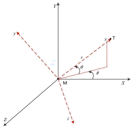
Figure 1.
Three-dimensional missile-target interception geometry.
Define and as the accelerations measured in the LOS frame for the target and the missile, respectively. According to the virtue of kinematics, the relative velocity between the missile and the target can be expressed as
According to the derivative rule of vector derivatives, we have
where and refers to the derivate of in and , respectively, and represents the rotation speed for relative to the inertial coordinate system . It can be acquired from Figure 1 that
By substituting Equations (1) and (3) into Equation (2), we can obtain
It should be noted that the collision course can be achieved with the LOS angle rate and converging to zero before hitting the target. Thus, Equations (5) and (6) are considered in the design of the guidance law.
Define , , , and the coupling state equations of LOS angles can be acquired as:
It can be concluded from Equation (7) that there exists cross-coupling between and . By virtue of the analysis in [1], and are small variables during the time horizon of the impact process. This gives . Moreover, the third order of the small variables can be neglected. Hence, Equation (7) can be rewritten as
The primary objective of the guidance law is to hit the target, which can be achieved with the convergence of the LOS angle rates converging to zero in both planes. Therefore, the objective is to design the guidance law that can zero the LOS angle rates before hitting the target.
3. Guidance Law Design
Considering the 3-D LOS angle motions are decoupled into two (2-D) LOS angular motions in the previous analysis, in this section, the planar fixed-time convergence guidance law is presented first. Then, the planar guidance law is further applied to the 3-D scenario. Although the decoupled model is utilized in the design of the 3-D guidance law, the proof for the convergence of LOS angle rates conducts on the cross-coupling model directly.
3.1. The Planar Guidance Law Design
In this subsection, the planar guidance law that can zero the LOS rate before hitting the target is proposed, and the decouple planar LOS motion of Equation (9) is considered in the design of the guidance law. Before deriving the guidance law, it is obliged to introduce some basic lemma of fixed-time stability theory.
Before deriving the guidance law, it is obliged to introduce some basic concepts of fixed-time stability theory [14].
Definition: The following nonlinear system is considered:
where the state and the upper semi-continuous mapping are denoted by and , respectively. The state is fixed-time stability if it is globally finite-time stable. Meanwhile, the function of the settling time is restricted by a real positive number i.e., . The definition can be stated mathematically as
Denote as the upper right-hand derivative of a function , . The fixed-time stability under the Lyapunov criterion is presented in Lemma 1.
Lemma 1.
Suppose a continuous positive definite and radially unbounded function as , such that:
for , then the origin is fixed-time stable for the system , and the settling time is given by:
Assume the deviations from the collision course for both the missile and target are small, then the relative velocity can be approximated as:
This assumption is reasonable since it can be conducted by a well-midcourse guidance process. Then, the instant range at time can be acquired as
Theorem 1.
If the guidance command can make the LOS angle rate satisfying:
where
, , , and
Then,
will converge to zero before hitting the target.
Proof.
The following continuously differential candidate function is considered:
The derivative of Equation (19) to time is
Substituting Equation (17) into Equation (20) yields
According to Lemma 1, will converge to zero in fixed-time. Define the settling time for as , then we have
Since in Equation (21) is a trivial case, assuming yields
Substituting Equation (13) into (23) yields:
Integrating the right side of Equation (24) from 0 to , and the corresponding integral interval for the left side is . One can obtain
Define
Substituting Equation (26) into (25) yields
Define as the final time of the engagement. According to Equation (16), one can obtain
Then, Equation (27) can be rewritten as
where merely relates to the initial LOS rate. Substituting Equation (22) into (26), one can further obtain
Thus, we can obtain . Combining Equations (29) and (30) yields , which implies that the convergence time for the LOS rate is always less than regardless of the initial conditions. Hence, the proof of Theorem 1 is completed. □
Substituting Equation (9) into (17) yields
Then, the guidance command is chosen a
where , and the additional term acts as the adaptive term to speed up the convergence process before hitting the target.
Theorem 2.
The guidance command in Equation (32) can zero the LOS angle rate before hitting the target.
Proof.
Substitute Equation (32) into (9), we have
By substituting Equation (33) into (17) yields
According to Theorem 1, the proposed guidance command in Equation (32) can lead to fixed-time convergence for the LOS angle rate, and the convergence rate increases as the value of m and n increases, or as the value of decreases. Hence, the proof of Theorem 2 is completed. □
3.2. Guidance Law Design in 3-D Engagement Scenario
According to the planar guidance law designed in the previous section, the fixed-time convergence guidance command for the 3-D engagement scenario can be designed as
Theorem 3.
The guidance commands in Equation (35) can achieve fixed-time convergence for the LOS angle rates in Equations (7) and (8) before hitting the target.
Proof.
The proof of Theorem 3 is divided into two parts. First, the effectiveness of the proposed guidance command under the condition is proven.
Substituting Equation (35) into (7) and (8) yields
The following continuously differential candidate function is considered:
The derivative of Equation (37) with respect to time is
Substituting Equation (36) into (38) yields
Since
Then, we can obtain
By choosing an appropriate inertial reference coordinate system, we can ensure that . Thus, . Then, Equation (41) can be rewritten as:
As we define in Theorem 1 that , we can further obtain
which can be written in an alternative form as
The proof for the proposed guidance command under the condition is similar; thus, it is omitted here. According to Theorem 1, the proposed guidance commands in Equation (35) can achieve fixed-time convergence for the LOS angle rate in Equations (7) and (8). Define as the convergence time in a 3-D scenario, the upper bound of the convergence time is given by
where is the upper bound for the settling time for the 3-D guidance scenario. It is obvious that is independent of the initial states. □
3.3. Discussion of the Potential Advantage of the Proposed Guidance Law
To facilitate the comparison between different guidance laws, the variable that needs to be restrained to zero during the guidance process is defined as . Some results on the design of guidance laws adopt the Lyapunov asymptotic stability theory as [6], the dynamic of is
Theoretically, the Lyapunov asymptotic stability theory only guarantees the convergence of when the time approaches infinity, and Equation (46) implies that when and only when , which means the convergence process of completes exactly at the instant of hitting the target. Some ideal assumptions are made during the design process of the guidance law. On the other hand, uncertainties and disturbances exist in practical applications. Hence, the error dynamic in Equation (46) may fail to converge to zero at the terminal instant in practical applications. Compared with the guidance law in [6], the proposed guidance law can ensure the convergence of before hitting the target, which makes it more robust to uncertainties and disturbances.
Some other results are based on the finite-time stability theory as [11], the convergence of can be completed in finite time, and the settling time satisfies
where and .
Compared with guidance laws based on the Lyapunov asymptotic stability theory, this group of guidance laws can achieve finite-time convergence of . However, the convergence upper bound in Equation (47) depends on initial states, and only a proper selection of the control parameter can ensure converged to zero before the final interception time. By contrast, the proposed guidance law can ensure convergence before hitting the target regardless of the initial conditions.
4. Simulations
In this section, numerical simulations are carried out to show the effectiveness of the proposed guidance laws. All the simulations are conducted on the Matlab platform via C++ programming. The simulation step is 0.01 s. All the simulations are terminated when the sign of the relative velocity becomes positive, or the relative range is less than 0.01 m.
4.1. Comparison Simulations
In this case, the comparison simulation is considered to show the effectiveness of the proposed guidance law. Detailed simulation parameters are tabulated in Table 1.

Table 1.
Initial states for the missile.
The performance of the proposed guidance law is compared with the finite-time convergence guidance law (FTCG) proposed in [9]. The guidance command for FTCG is given by
where , , .
Two different control parameters are selected for the comparison law. Detailed control parameters, in this case, are summarized in Table 2.
Table 2.
Control parameters for guidance laws.
Simulation results for both guidance laws are shown in Figure 2. Dot lines represent the results of the proposed guidance law. Dash lines and solid lines represent the results for FTCG under two different control parameters. Figure 2a shows the elevation acceleration, and Figure 2b represents the profile of the elevation LOS angle rate. Figure 2c shows the azimuth acceleration, and Figure 2d represents the profile of the azimuth LOS angle rate.
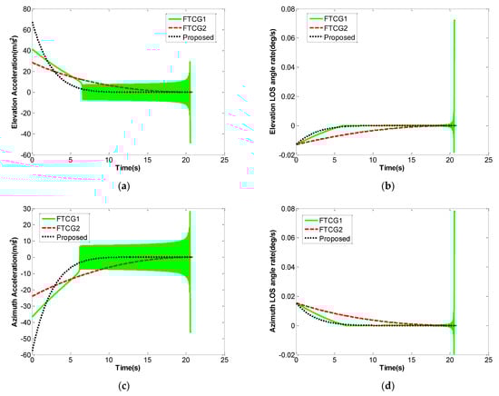
Figure 2.
Comparison results. (a) Elevation acceleration. (b) Elevation LOS angle rate. (c) Azimuth acceleration. (d) Azimuth LOS angle rate.
Although each guidance law can impact the target successfully, the acceleration variation and the convergence of the LOS angle rate are significantly different. The acceleration for the proposed guidance law converges to zero in fixed time and remains there afterward, while the comparison law with the first group of control parameters will fluctuate around zero until the instant of impact, as demonstrated by FTCG1. There would be no chattering for the proposed guidance law under any allowable control parameters. As a result, the proposed guidance law can achieve higher accuracy than the comparison law. However, the comparison law can avoid chattering by proper selection of control parameters, as FTCG2 does. However, the LOS angle rate only converges to zero at the end of the impact, failing to exhibit the characteristic of finite-time convergence. Hence, the proposed guidance law has better performance than the comparison law.
4.2. Simulations with Autopilot Dynamics
As shown in the previous simulation case, the initial acceleration for the missile under the proposed law is very large. However, acceleration usually grows from scratch in practice. Furthermore, the autopilot delays are uncompensated during the design of the guidance law. Hence, it is necessary to investigate the performance of the proposed guidance law under the effect of autopilot dynamics.
Some existing methods compensate for the autopilot dynamics by computing the control parameter at each time step in a feedback manner, which makes the guidance law more complicated. Since robustness is a generic characteristic of the proposed guidance law, the control parameters do not need to be calculated in a feedback-step manner. To show the robustness of the proposed guidance laws, a first-order autopilot dynamic is considered in this simulation, which can be expressed as
where is the ideal acceleration, is the actual acceleration. The time constant considered for the autopilot dynamic, in this case, is 0.5. Initial conditions and control parameters are the same as in the previous section.
Simulation results are shown in Figure 3. Ideal and actual accelerations are plotted with different types of lines in Figure 3a,c. It is obvious that there exists a tracking error between the ideal and actual accelerations under the effect of autopilot delays. However, this error can be eliminated in a fixed time without extra effort under the proposed guidance law. Simulation results with actual command are plotted in blue solid line in Figure 3b,d, which converge to zero before the final time and ensure the successful impact of the target. Even though the proposed guidance law is derived from a lag-free system, the guidance law can provide high accuracy in a realistic missile system with autopilot lag.
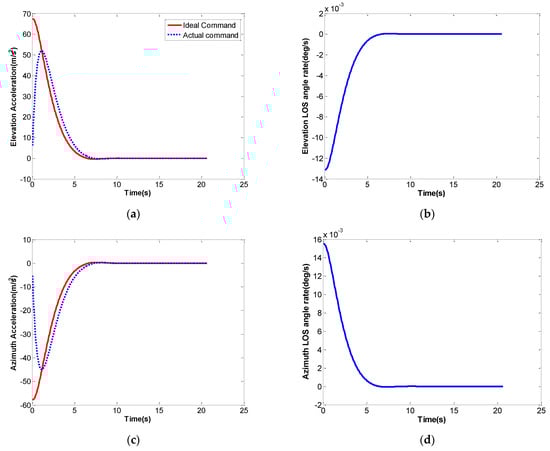
Figure 3.
Simulation with autopilot dynamics. (a) Elevation acceleration. (b) Elevation LOS angle rate. (c) Azimuth acceleration. (d) Azimuth LOS angle rate.
4.3. Simulations with Different m and n
In this case, the performance of the proposed guidance law in a 3-D Scenario is studied under different control parameters, which are , , .
Simulation results are shown in Figure 4 and Figure 5. Solid lines, dash lines, and dot lines represent the results for three different control parameters. Figure 4a shows the elevation acceleration, and Figure 4b represents the profile of the elevation LOS angle rate. Figure 5a shows the azimuth acceleration, and Figure 5b represents the profile of the azimuth LOS angle rate.
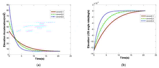
Figure 4.
Simulation results in the elevation plane with different m and n. (a) Elevation acceleration. (b) Elevation LOS angle rate.
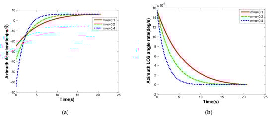
Figure 5.
Simulation results in the azimuth plane with different m and n. (a) Azimuth acceleration. (b) Azimuth LOS angle rate.
For all the various values of control parameters, the LOS angle rate can converge to zero in fix time, as shown in Figure 4b and Figure 5b. The collision course can be achieved, and the impact of the target can be ensured. Moreover, the miss distance for the missile can be less than 0.1 m. It also can be concluded from Figure 4b and Figure 5b that the convergence rate for the LOS angle rate increases as the value of the control parameter increases. This is in line with Theorem 3. However, a higher convergence rate requires larger guidance commands at the beginning of the guidance process, as is demonstrated in Figure 4a and Figure 5a.
4.4. Simulations with Different γ
In this case, the initial conditions for the missile and the initial coordinates for the target are the same as in Section 4.1. The speed for the target is = 200 m/s, and the acceleration is = 6 m/s.
Simulation results are shown in Figure 6 and Figure 7. Solid lines, dash lines, and dot lines represent the results for three different control parameters. Figure 6a shows the elevation acceleration, and Figure 6b represents the profile of the elevation LOS angle rate. Figure 7a shows the azimuth acceleration, and Figure 7b represents the profile of the azimuth LOS angle rate. The collision course is achieved with the LOS angle rate converging to zero. It is clear from Figure 6b and Figure 7b that the convergence of the LOS angle rate achieves in fixed time for all the control parameters. It also can be concluded from Figure 6b and Figure 7b that the convergence rate for the LOS angle rate increases as the value of the control parameter decreases. This is in line with Theorem 3. Moreover, a higher convergence rate requires larger guidance commands at the beginning of the guidance process, as is demonstrated in Figure 6a and Figure 7a.
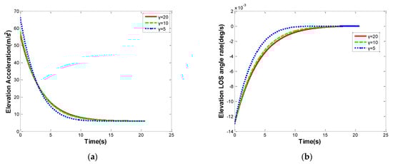
Figure 6.
Simulation results in the elevation plane with different γ. (a) Elevation acceleration. (b) Elevation LOS angle rate.
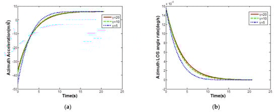
Figure 7.
Simulation results in the azimuth plane with different γ. (a) Azimuth acceleration. (b) Azimuth LOS angle rate.
5. Conclusions
Novel fixed-time convergence guidance laws are proposed for diverse engagement scenarios, and the fixed-time convergence of the LOS angle rate is proven under the proposed laws. The convergence rate is merely related to control parameters, a suitable selection of which can ensure the convergence is fulfilled before the final impact time. Unlike finite-time convergence guidance law, the proposed method is not affected by the chattering effect. The simulation results present high accuracy in a realistic missile system for autopilot first-order time constants as high as 0.5 s. In our future related research, more constraints to improve the missile performance should also be concerned, such as impact time and impact angle.
Author Contributions
Conceptualization, Y.L. and Z.C.; Methodology, Y.L. and Z.C.; Formal analysis, Z.C.; Investigation, C.O., C.S. and Z.C.; Data curation, C.O.; Writing—review & editing, C.S. All authors have read and agreed to the published version of the manuscript.
Funding
This study was co-supported in part by the National Natural Science Foundation of China (No. 61903146).
Data Availability Statement
Not applicable.
Conflicts of Interest
The authors declare no conflict of interest.
References
- Zarchan, P. Tactical and Strategic Missile Guidance, 6th ed.; American Institute of Aeronautics & Astronautics Inc.: Reston, VA, USA, 2012; pp. 569–600. [Google Scholar]
- Yang, C.D.; Chen, H.Y. Three-dimensional nonlinear H∞ guidance law. Int. J. Robust Nonlinear Control 1999, 32, 3079–3084. [Google Scholar]
- Liao, F.; Luo, Q.; Ji, H.; Gai, W. Guidance laws with input saturation and nonlinear robust H∞ observers ☆. ISA Trans 2016, 63, 20–31. [Google Scholar] [CrossRef] [PubMed]
- Lechevin, N.; Rabbath, C.A. Lyapunov-Based Nonlinear Missile Guidance. J. Guid. Control Dyn. 2004, 27, 1096–1102. [Google Scholar] [CrossRef]
- Saleem, A.; Ratnoo, A. Lyapunov-Based Guidance Law for Impact Time Control and Simultaneous Arrival. J. Guid. Control Dyn. 2015, 39, 164–173. [Google Scholar] [CrossRef]
- Cheng, Z.; Liu, L.; Wang, Y. Lyapunov-based switched-gain impact angle control guidance. Chin. J. Aeronaut. 2018, 31, 765–775. [Google Scholar] [CrossRef]
- Cheng, Z.; Bo, W.; Lei, L.; Wang, Y. A composite impact-time-control guidance law and simultaneous arrival. Aerosp. Sci. Technol. 2018, 80, 403–412. [Google Scholar] [CrossRef]
- Liu, W.; Wei, Y.; Duan, G. Barrier Lyapunov function-based integrated guidance and control with input saturation and state constraints. Aerosp. Sci. Technol. 2019, 84, 845–855. [Google Scholar] [CrossRef]
- Zhou, D.; Sun, S.; Teo, K.L. Guidance Laws with Finite Time Convergence. J. Guid. Control Dyn. 2009, 32, 1838–1846. [Google Scholar] [CrossRef]
- Zhao, Z.; Li, C.; Yang, J.; Li, S. Output feedback continuous terminal sliding mode guidance law for missile-target interception with autopilot dynamics. Aerosp. Sci. Technol. 2019, 86, 256–267. [Google Scholar] [CrossRef]
- Sun, S.; Zhou, D.; Hou, W.T. A guidance law with finite time convergence accounting for autopilot lag. Aerosp. Sci. Technol. 2013, 25, 132–137. [Google Scholar] [CrossRef]
- Kumar, S.R.; Rao, S.; Ghose, D. Sliding-Mode Guidance and Control for All-Aspect Interceptors with Terminal Angle Constraints. J. Guid. Control Dyn. 2012, 35, 1230–1246. [Google Scholar] [CrossRef]
- Kumar, S.R.; Rao, S.; Ghose, D. Nonsingular Terminal Sliding Mode Guidance with Impact Angle Constraints. J. Guid. Control Dyn. 2014, 37, 1114–1130. [Google Scholar] [CrossRef]
- Polyakov, A. Nonlinear Feedback Design for Fixed-Time Stabilization of Linear Control Systems. IEEE Trans. Autom. Control 2012, 57, 2106–2110. [Google Scholar] [CrossRef]
- Zhang, Y.; Tang, S.; Guo, J. An adaptive fast fixed-time guidance law with an impact angle constraint for intercepting maneuvering targets. Chin. J. Aeronaut. 2018, 31, 1327–1344. [Google Scholar] [CrossRef]
- Li, G.; Wu, Y.; Xu, P. Fixed-time cooperative guidance law with input delay for simultaneous arrival. Int. J. Control 2021, 94, 1664–1673. [Google Scholar] [CrossRef]
- Zhang, P.; Zhang, X. Multiple missiles fixed-time cooperative guidance without measuring radial velocity for maneuvering targets interception. ISA Trans. 2021, 126, 388–397. [Google Scholar] [CrossRef]
- Chen, Z.; Chen, W.; Liu, X.; Cheng, J. Three-dimensional fixed-time robust cooperative guidance law for simultaneous attack with impact angle constraint. Aerosp. Sci. Technol. 2021, 110, 106523. [Google Scholar] [CrossRef]
- Liu, J.; Zhang, Y.; Liu, H.; Yu, Y.; Sun, C. Robust eventtriggered control of second-order disturbed leader-follower mass: A nonsingular finite-time consensus approach. Int. J. Robust Nonlinear Control 2019, 29, 4298–4314. [Google Scholar] [CrossRef]
- Wang, H.; Zhu, Q.X. Finite-time stabilization of high-order stochastic nonlinear systems in strict-feedback form. Automatica 2015, 54, 284–291. [Google Scholar] [CrossRef]
- Zuo, Z.; Tie, L. A new class of finite-time nonlinear consensus protocols for multi-agent systems. Int. J. Control 2014, 87, 363–370. [Google Scholar] [CrossRef]
- Zuo, Z.; Tie, L. Distributed robust finite-time nonlinear consensus protocols for multi-agent systems. Int. J. Syst. Sci. 2016, 47, 1366–1375. [Google Scholar] [CrossRef]
- Yu, J.; Yu, S.; Li, J.; Yan, Y. Fixed-time stability theorem of stochastic nonlinear systems. Int. J. Control 2019, 92, 2194–2200. [Google Scholar] [CrossRef]
- Li, H.; Li, C.; Huang, T.; Ouyang, D. Fixed-time stability and stabilization of impulsive dynamical systems. J. Frankl. Inst.-Eng. Appl. Math. 2017, 354, 8626–8644. [Google Scholar] [CrossRef]
- Liu, J.; Zhang, Y.; Yu, Y.; Sun, C. Fixed-time event-triggered consensus for nonlinear multiagent systems without continuous communications. IEEE Trans. Syst. Man Cybern.-Syst. 2021, 49, 2221–2229. [Google Scholar] [CrossRef]
Disclaimer/Publisher’s Note: The statements, opinions and data contained in all publications are solely those of the individual author(s) and contributor(s) and not of MDPI and/or the editor(s). MDPI and/or the editor(s) disclaim responsibility for any injury to people or property resulting from any ideas, methods, instructions or products referred to in the content. |
© 2023 by the authors. Licensee MDPI, Basel, Switzerland. This article is an open access article distributed under the terms and conditions of the Creative Commons Attribution (CC BY) license (https://creativecommons.org/licenses/by/4.0/).