Abstract
Soft computing models based on fuzzy or probabilistic approaches provide decision system makers with the necessary capabilities to deal with imprecise and incomplete information. Hybrid systems based on different soft computing approaches with complementary qualities and principles have also become popular. On the one hand, fuzzy logic makes its decisions on the basis of the degree of membership but gives no information on the frequency of an event; on the other hand, the probability informs us of the frequency of the event but gives no information on the degree of membership to a set. In this work, we propose a new measure that implements both fuzzy and probabilistic notions (i.e., the degree of membership and the frequency) while exploiting the ability of the convolution operator to combine functions on continuous intervals. This measure evaluates both the degree of membership and the frequency of objects/events in the design of decision support systems. We show, using concrete examples, the drawbacks of fuzzy logic and probability-based approaches taken separately, and we then show how a fuzzy probabilistic convolution measure allows the correction of these drawbacks. Based on this measure, we introduce a new clustering method named Fuzzy-Probabilistic-Convolution-C-Means (FP-Conv-CM). Fuzzy C-Means (FCM), Probabilistic K-Means (PKM), and FP-Conv-CM were tested on multiple datasets and compared on the basis of two performance measures based on the Silhouette metric and the Dunn’s Index. FP-Conv-CM was shown to improve on both metrics. In addition, FCM, PKM, and FP-Conv-CM were used for multiple image compression tasks and were compared based on three performance measures: Mean Square Error (MSE), Peak Signal-to-Noise Ratio (PSNR), and Structural SImilarity Index (SSIM). The proposed FP-Conv-CM method shows improvements in all these three measures as well.
MSC:
60xx; 03xx
1. Introduction
Thanks to their ability to simulate human reasoning, fuzzy and probabilistic models allow the construction of automatic decision makers capable of handling very complex phenomena using limited knowledge, in particular for clustering, which is an unsupervised learning task consisting of grouping a collection of elements into subgroups so that the elements in the same group are more similar (according to a certain measure) compared with the objects in other groups. Clustering plays a critical role in data mining and as a standard method for statistical data analysis. It is widely employed in various tasks in machine learning, pattern recognition, image analysis, information retrieval, bioinformatics, data compression, and computer graphics. In this work, we introduce a new clustering method named Convolution-Fuzzy-Probabilistic-C-Means (FP-Conv-CM) that implements a new sub-measure, and which is a hybrid of two soft computing approaches: fuzzy logic and probabilistic methods.
The fact that the term “cluster” is not precisely defined is one reason behind the existence of numerous clustering methods. One thing they all have in common is the grouping of data objects. Nevertheless, many researchers have developed and employed various cluster models, and, again, several methods may be provided for each of these cluster models. Typical cluster models include connectivity models [1], centroid models [2], distribution models, density-based clustering [3], subspace models [4,5], graph-based models [6], and neural clustering models [7].
Clustering methods can be roughly distinguished into hard clustering or soft clustering methods. There are more specific distinctions that can be discussed, including (a) hierarchical clustering [8] (a child cluster’s objects are likewise a part of the parent cluster); the hierarchy can be built either by dividing or merging recursively [9,10], (b) strict partitioning clustering with and without outliers (objects might belong to none, which is referred as outliers); the partition-based clustering technique divides the data points of a dataset into different partitions [11,12,13], (c) overlapping clustering techniques, where an object may belong to one or more clusters; partitioning algorithms that overlap include the commonly used Fuzzy K-means and its variations [14,15], (d) subspace clustering (i.e. while an overlapping clustering, within an individually defined subspace, clusters are not expected to overlap) [16,17]. Fuzzy clustering is one of the most established clustering methods that partition the dataset into overlapping clusters, i.e., each object belongs to several clusters with different degrees of membership [18]. The notion of membership function embodies the concept of fuzzy sets and fuzzy logic. The effectiveness of soft clustering has been confirmed when dealing effectively with the discrimination of datasets in n-dimensional spaces and is more useful for unlabeled data and datasets with outliers.
Dunn presented the widely used Fuzzy C-mean algorithm (FCM) [18], and over the years, Bezdek [19] has suggested an improved version of FCM; this algorithm being the soft centroid-based model that allows one piece of data to belong to two or more clusters. Due to the poor performance of FCM against noise and intensity inhomogeneity, many variants of FCM have been developed. These FCM variations are covered in [20]. FCM fails to discriminate between data points and noise or outliers, thus centroids could be stuck in the outliers instead of in the centers. To overcome this drawback, ref.[21] proposed a possibilistic C-means algorithm, where PCM is a distribution-based model which assumes that the observations of the learning set are the realizations of a random variable whose density function is a mixture of normal distributions [22] where the membership is the degree of belonging that illustrates how the datum is compatible with the class typicality. This makes it possible to improve performance when dealing with noise and outliers. Despite its capability, the PCM is sensitive to initializations and choices of parameters, it can generate coincident clusters, and also suffers from the degenerescence problem, i.e., when some group is empty, the standard deviation tends toward 0 [23]. To correct that, Pal et al. [24] combined FCM and PCM while considering the need for both relative and absolute typicalities in clustering. Another weakness of the possibilistic C-means is the negligence of membership values even with the observation of the typicality values. Further variants of the PCM method have been enhanced by changing the objective function to address some of the PCM’s shortcomings [25,26,27].
Furthermore, there are many attempts to benefit from the combination of FCM and the possibilistic approach to ameliorate the results, also recognizing the requirement for applying membership and typicality values simultaneously [24,28,29]. Once more, Pal et al. [30] presented a new impressive model named Possibilistic Fuzzy C-means (PFCM), which simultaneously created, for each cluster, a membership and typicity values with the standard prototypes or cluster centers. This algorithm has resolved the primary overlap and coincidence cluster issues that plagued PCM, in addition to removing noise sensitivity issues in FCM. Unfortunately, all these algorithms did not give satisfactory results, thus it was better to use a new approach [31] that enhanced the PFCM model to precisely detect the cluster centers. The authors introduced the Modified Possibilistic Fuzzy C-Means (MPFCM) with norm functions, including the covariance norm, thus making it superior and flexible at correcting the most complicated problems that other variants find challenging—mainly noise issues and outlier points.
Several other clustering methods have been created in order to prove the possibility that a data point might belong to multiple sub-clusters at once, and some of these algorithms were based on neutrosophic logic. In [32], a Neutrosophic C-means algorithm (NCM) was presented to derive such an approach by introducing a new objective function handling two different classes of rejection—the ambiguity rejection and the distance rejection—to correct the FCM method’s weakness in identifying noise and outlier data points. NCM simultaneously calculates the degrees of belonging to the determinate and indeterminate clusters for each of the data points. By using a new iterative process, Guo and Sengur [33] updated the membership degrees to the ambiguity and outlier class of data points, and as a result, the membership functions are more immune to noise. The study [34] suggested a new Kernel NCM clustering algorithm (KNCM) to improve the idea of the NCM approach for nonlinear-shaped data clustering by combining the kernel function with the neutrosophic logic. In addition, they produced a novel cost function to solve for noise and outliers using a robust parameter estimation, which led to generation of a new membership function and prototype update equations. Along the same lines, [35] proposed a new kernel-based fuzzy clustering method to deal with the issue of arbitrary cluster shapes. A novel utilization of the kernel method was proposed to extract more expressive features implicitly and may be used to reduce the struggle during fuzzy clustering of high dimensional data by discovering good new representations from the original data. The kernel approach in [36] has emerged as an interesting and quite viable alternative to fuzzy clustering. In addition, [37] proposed multiple kernel fuzzy clustering (MKFC), which expands the fuzzy c-means algorithm with the multiple kernel-learning setting. MKFC has more excellent resistance to useless features and kernels by employing multiple kernels and an automated adjustment of the kernel weights. A multiple kernel fuzzy c-means (MKFCM) approach was also presented by [38], who developed a novel algorithm that uses a linear composite of multiple kernels and automatically determines the updating of the linear coefficients of the combined kernel.
Fuzzy clustering plays an important role in the field of data mining. Since the membership function offers a powerful tool for the identification of changing class structures, ref.[39] has suggested a technique for dynamic data mining that focuses on fuzzy c-means. This approach appears to afford a convenient method for the detection of changing class structures. Unfortunately, it suffers from several weaknesses, and [40] proposed some adjustments that led to the creation of the modified dynamic fuzzy c-means (MDFCM) algorithm. This allows for more flexibility in membership function estimation and averts the use of extremely complicated equations [41]. In a recent paper, we developed a clustering model based on a recurrent neural network, an optimization model that treats various samples equally, and the Euler-Cauchy technique with a fixed time step [42]. However, outlier samples make it impossible to identify the true groups and cause a very long and incorrect convergence trajectory. We investigated, in [43], a constrained optimization method that de-assigns memberships from centers to reduce the impact of outlier samples. To benefit from the capacity of dynamic systems to memorize prior groupings and the understanding of the features of the data by neural networks, we have introduced, in our previous work [44], an original clustering method that implements fuzzy logic and a recurrent neural network, namely the Recurrent Neural Network Fuzzy C-means. Other recent versions of Fuzzy C-means were introduced. In [45], authors proposed a gradient descent algorithm based on possibilistic fuzzy c-means for clustering noisy data. In [46], authors suggested the Optimization of a Fuzzy C-Means Clustering Algorithm with a Combination of Minkowski and Chebyshev Distance Using Principal Component Analysis. Wang et al. introduced an improved index for clustering validation based on the Silhouette index and the Calinski–Harabasz index [47]. A hybrid fuzzy c-means clustering algorithm was suggested in [48] and was essentially focused on big data problems. The Deep Possibilistic C-means Clustering Algorithm was recently introduced by Gu Y et al. and was used on medical datasets [49].
In this work, we propose a new sub-measure that implements both notions (the degree of membership and the frequency of “pattern p belongs to A with degree of membership (A,p)”, event denoted with an E, while exploiting the ability of the convolution operator to combine functions on continuous intervals. This measure evaluates both the degree of membership and the frequency of E in the design of decisional systems. We show, using concrete examples, the disadvantages of fuzzy logic and probability-based approaches taken separately, and then we show how a convolution probabilistic measure allows the correction of these disadvantages. Based on this measure, we introduce a new clustering method named Fuzzy-Probabilistic-Convolution-C-Means (FP-Conv-CM). FCM, PKM, and FP-Conv-CM were comparatively tested on several datasets to analyze the clustering task and on several images to analyze the compression task. FCM, PKM, and FP-Conv-CM were compared based on several performance measures: Silhouette and Dunn’s indexes, mean square error, structural similarity (SSIM), and peak signal-to-noise ratio (PSNR). Considering the results obtained using FCM and PKM, FP-Conv-CM was able to improve the Silhouette and Dunn’s Indexes. In addition, FP-Conv-CM improved MSE, PSNR, and SSIM values.
The rest of the paper is organized as follows: In Section 2, we present the methodology adopted in this work to achieve the stated goals. In Section 3, we discuss the disadvantages of fuzzy and Probabilistic K-means using concrete data. In Section 4, the proposed fuzzy probability measure is described and used for clustering tasks. In Section 5, we present experimental results, and Section 6 concludes the paper.
2. Methodology Overview
Let represent the space of unlabeled observations. The clustering methods seek to reduce the information contained in :
- By summing it up as a set , where ; these vectors will be called referents (centers) throughout the rest of the article;
- By defining an assignment function, χ, which is an application of in the set of indices , this function makes it possible to realize a partition of in subsets, .
It should be noted that the clustering problem is NP difficult. Indeed, if (the number of groups) and (the dimension), are fixed and is the number of items to be clustered, then the problem can be solved exactly in time [50].
Definitions
- Data is the dataset under study;
- Centers is the set of the centers to be determined;
- is the allocation function of data to the groups represented by the centers ;
- , are the groups determined based on ;
- is the membership function of group where m is a real number strictly greater than 1;
- is the probability of x being in group , where is the covariance of the component .
The quantity measures the frequency that is taken from ; whereas measures the degree of belonging of to . Our idea is to define a new borelian measure that measures the degree of belonging of to with frequency.
Methods
In this work, we introduce a new measure that measures the degree of belonging of to with frequency. This measure is called fuzzy probability convolution measure and implements the following membership-density functions:
For a continuous case:
For a discrete case:
Based on the proposed fuzzy probability convolution measure, we introduce a new clustering method that we named Fuzzy Probabilistic Convolution C-Means (FP-Conv-CM). This method estimates the vectors , the common standard deviation , and the membership coefficients. Based on FP-Conv, the model implementing these parameters must approximate the true density that generated the data . In this regard, our method involves maximizing the fuzzy probability of the observations:
where represents the likelihood measuring the capacity of the model to reproduce the data , is the matrix of the membership coefficients (which represents the degree of membership of each data to each group ), and is the group that won the sample according to FP-Conv.
Metrics
One of the biggest challenges facing researchers is how to evaluate the clustering. The homogeneity of the created classes/clusters and the separation between them are calculated in order to assess the efficiency of the clustering method. These qualities may be evaluated using a variety of indices:
- Silhouette index:
- Let N be the number of patterns. The Silhouette index [43] finds the optimal clustering effect using the difference between the average distance within the cluster and the minimum distance between the clusters, i.e., the silhouette coefficient is given as follows:
- represents the average distance from sample to other samples in the cluster;
- represents the minimum distance from sample to the other clusters.
- The silhouette coefficient ranges from −1 to 1, where −1 denotes that the data point is not assigned to the relevant cluster, 0 denotes that the clusters are overlapping, and 1 denotes that the cluster is dense and well-separated. This metric is one of the most popular measurements in clustering. It can distinguish between objects that were placed wisely within their cluster and those that are in the outlier zone between clusters.
- Dunn index: The Dunn index [40,44] is defined as
If and are different clusters then is the minimal distance between samples in different clusters and is the largest within-cluster distance. Note that large inter-cluster distances (better separation) and smaller cluster sizes (more compact clusters) lead to higher DI values. A higher DI value implies better clustering [40]. It assumes that better clustering means that clusters are compact and well-separated from other clusters.
The performance measures used to evaluate different image compressions are:
- (a)
- Mean Squared Error (MSE), which calculates the error between the initial image and the compressed image. It is in fact the distance between two matrices that represent the images to be compared.
- (b)
- Peak Signal-to-Noise Ratio (PSNR), which implements the following equation:where peakval is taken from the range of the image datatype.
- (c)
- Structural SIMilarity (SSIM) index, which is calculated on various windows of an image. The measure between two windows x and y of common size is:
Where , is the variance of , and is the covariance of and ; and are two constants estimated from the image [51].
Experimental validation
FCM, PKM, and FP-Conv-CM were tested on multiple datasets and compared on the basis of two performance measures, i.e., the Silhouette metric and Dunn’s Index (see Section 5.2). FP-Conv-CM was able to improve the Silhouette value by 1000 and Dunn’s Index by 0.024.
FCM, PKM, and FP-Conv-CM were used for multiple image compression tasks and were compared based on three performance measures: mean squared error (MSE), peak signal-to-noise ratio (PSNR), and structural similarity index (SSIM) (see Section 5.3). FP-Conv-CM improved MSE by 3000, PSNR by 11, and SSIM by 0.32.
3. Drawbacks of Fuzzy and Probabilistic Approaches
3.1. K-Means
The K-means method, which is the most well-known vector quantization method, determines the set of reference vectors and the assignment function , by minimizing the cost function:
The time complexity of K-means is [52], where is the number of iterations needed until convergence. The k-means method suffers from several drawbacks due to it being a hard clustering method. To overcome these issues, there exist many extensions, including FCM and PKM [43].
3.2. Probabilistic K-Means
To obtain the probabilistic version of k-means, it is assumed that the observations of the learning set are the realizations of a random variable whose density function is a mixture of normal distributions [44,53]:
where ; and is the normal density function.
In addition to this formalism, the shift to the probabilistic interpretation of the K-means algorithm requires us to introduce additional assumptions:
- The prior probabilities are all equal to ;
- The k normal functions have identical variance–covariance matrices equal to , where represents the unit matrix and is the standard deviation considered constant for all these normal distributions.
- In that case, the density function has the following expression:
- The k-means probabilistic version involves estimating the vectors and the typical standard deviation trying to realize the sample as much as possible. This method, known as the maximum likelihood method, involves maximizing the probability of these observations.
- Maximizing the classifying likelihood amounts to minimizing:
- Probabilistic k-means has a running time of [52], where is the number of -dimensional vectors, is the number of clusters, and is the number of iterations required to reach convergence; CONST is a constant that depends only on the data.
3.3. Fuzzy C-Means (FCM)
The fuzzy mean square clustering algorithm known as Fuzzy C-means (FCM) allows one sample of data to belong to each cluster with different degrees of membership. This method is frequently used in pattern recognition [42]. The objective function of the FCM method is minimizing the following error:
where the real value determines the fuzziness of the generated clusters (m > 1), is the dataset size, is the number of clusters, is the degree of membership of sample to the cluster , is the -dimensional center of the cluster , and ‖.‖ represents any norm denoting the similarity between each measured data and the center.
An iterative optimization of the objective function presented above is used to perform a fuzzy partitioning, with the update of membership and the cluster centers by:
This iteration will stop when , where is a termination criterion between 0 and 1, whereas are the iteration steps. This procedure converges to a local minimum or a saddle point of .
3.4. Fuzzy Reasoning and Probabilistic Reasoning Are Complementary
Let be a set from . The probability, measures the probability that is taken from , whereas measures the degree of belonging of to .
Probabilistic reasoning corrects the weakness in fuzzy reasoning:
Consider a dataset whose elements are distributed according to two normal distributions, and , presented in Figure 1.
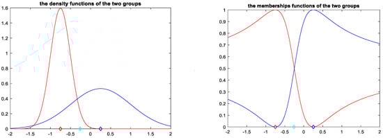
Figure 1.
Fuzzy membership functions and probability densities of two clusters associated with N1 and N2 red color corresponds to the first group and the blue one corresponds to the second color.
These two distributions form two clusters (or classes), namely C1 and C2. In this subsection, we will use probabilistic and fuzzy models to recognize the classes of some critical data. When we generated the data, we noticed that some samples have a very high frequency and are not close enough to the centers of the two densities. As we will see later, depending on the case study, this type of data misleads both models.
Example 1.
We consider the element , of high frequency, from class (or cluster) C2.
- (a)
- The fuzzy model based on the membership functions and , presented in Figure 1, predicts as an element of C1.
In fact, we have and then and thus, the fuzzy model predicts that the sample is from class 1 with center , which is false.
- (b)
- The probabilistic model based on the densities and , presented in Figure 1, predicts as an element of C2
In fact, we have and .
Thus, the probability model predicts that s is from class 2 with center , which is true.
Fuzzy reasoning corrects the weakness in probabilistic reasoning:
Consider a dataset whose elements are distributed according to two normal distributions, and . These two distributions form two clusters (or classes), namely C1 and C2. In this subsection, we will use probabilistic and fuzzy models to recognize the classes of some critical data. When we generated the data, we noticed that some samples are close to the mean of the two densities and do not have a very high frequency. As we will see later, this perturbs the decision of the models.
Example 2.
We consider the element , close to the center 0, of the class (or cluster) C1.
- (a)
- The fuzzy model based on the membership functions and given below predicts as an element of C1.
In fact, we have and , thus, the fuzzy logic predicts that the sample is from class 1 with center , which is true.
- (b)
- The probabilistic model based on the membership functions and given below predicts as an element of C2.
In fact, we have and .
Thus, the probability approach predicts that is from class 2 of center , which is false.
Drawbacks of fuzzy and probabilistic approaches on real data: image compression case study:
To show the limits of fuzzy and probabilistic approaches on real data, we have used these methods to compress images and we have conducted a deep analysis of the obtained results. For this, we have used the image of the great scientist Max Planck (see Figure 2a). The histogram of this image is given in Figure 2b, while Figure 2c highlights an ambiguous pixel.
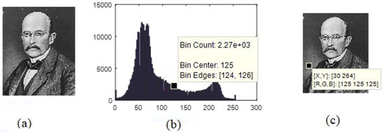
Figure 2.
(a) Max Planck. (b) Histogram of the Max Planck image, and (c) pixel mid-distance of the two fuzzy centers.
The image obtained after decompression is shown in Figure 3a (after compression using 2-GMM). The histograms of group 1 (center = 58.95, std = 15.98) and group 2 (center = 58.95, std = 15.98), obtained using 2-GMM, are given in Figure 3b,c, respectively.
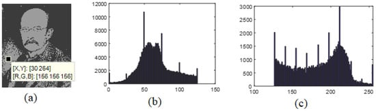
Figure 3.
(a) Decompression of the image of Max Planck compressed using 2-GMM. (b) The histogram of group 1 pixels obtained using 2-GMM (center = 58.95, std = 15.98), and (c) the histogram of group 2 pixels obtained using 2-GMM (center = 155.61, std = 50.04).
The image obtained after decompression is shown in Figure 4a (following compression using 2-FCM). The histograms of group 1 (center 1 = 63.75) and group 2 (center 2 = 186.53), obtained using 2-FCM, are given in Figure 4b,c, respectively.
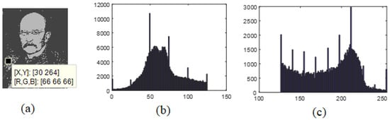
Figure 4.
(a) Decompression of the image of Max Planck compressed using 2-FCM. (b) Histogram of group 1 pixels obtained using 2-FCM (center 1 = 63.75), and (c) histogram of group 2 pixels obtained using 2-FCM (center 2 = 186.53).
In the first phase of this example, we focus on the pixels with a gray level 125, which represent 29.05% of the image; for example, the pixel located at position [30 264], which is called p. For pedagogical reasons, we have highlighted this pixel on the different histograms and the different images of Max Planck—original and those obtained by decompression.
This kind of pixel causes ambiguities for 2-FCM, but 2-GMM assigns them correctly thanks to amplification of the small quantities (thanks to the averages and standard deviations) by the exponential function of each Gaussian component.
Indeed, the degrees of membership of p to each of these groups, formed by 2-FCM, are given by et ; thus . The probabilities of p belonging to each of the two groups formed using 2-GMM are given by and ; hence, the clarity of the probabilistic decision with respect to the suitable group of the pixel p.
In the second phase of this example, we focus on the pixels with a gray level of 92, which represent 45.8% of the image; for example, the pixel located at position [198 279], which is called q. This kind of pixel causes ambiguities for 2-GMM, but 2-FCM assigns them correctly thanks to the integration of all centers in the formulas of all membership functions.
Indeed, the probabilities of q belonging to each of the two groups are et ; thus . The degree of membership of q in each of these groups formed by 2-FCM are given by and ; hence the clarity of the fuzzy decision with respect to the suitable group of pixel q.
In the next section, in order to overcome these shortcomings, we will introduce a hybrid sub-measure that implements both fuzzy and probabilistic concepts.
4. Proposed Approach
4.1. Fuzzy Probability Convolution Measure
Our idea is to define a new hybrid measure that implements the fuzzy and the probability reasonings at the same time and corrects the shortcoming of the classical reasoning. Thus, this new measure computes the frequency of taking from and the degree of belonging of to at the same time; we call this measure fuzzy probability convolution.
Definition 1.
(Convolution-Fuzzy-probability): The Fuzzy Probability Convolution (FP-Conv) measure is defined based on the convolution of the membership function and on the density (probability) as given by:
For a continuous case:
For a discrete case:
The fuzzy probability convolution corrects the incorrect decisions of the fuzzy logic.
Consider the following membership functions:
and the following normal density functions:
Proposition 1.
Based on the decision model implementing the following FP-Conv densities:
and , the sample is predicted as the element of class 2, which is true.
Proof.
We have 0.055585, and ; thus, .
Thus, is considered as an element of the class with center , which is true.
Note:
It should be noted thatand , which means that the decision is clearer. □
The convolution fuzzy probability corrects the incorrect decisions of the probability reasoning.
Consider the membership functions and, and the normal densities functions and .
Proposition 2.
Based on the fuzzy density measures and , the sample is predicted as an element of class 1, which is true.
Proof.
We have and; thus .
Thus, is predicted as an element of the class with center , which is true.
Note:
It should be noted that and . □
4.2. Fuzzy Probabilistic Convolution C-Means
The quantity measures the frequency that is taken from ; whereas, measures the degree of belonging of to . Our idea is to define a new borelian measure that measures the degree of belonging of to with frequency. This new measure calculates the frequency of taking from and the degree of belonging of to at the same time.
Based on the concepts introduced in Section 2, the fuzzy probability convolution clustering method implements the following membership density functions:
Continuous case:
Discrete case:
The following example shows, geometrically, how the new membership density function makes the decision increasingly clearer and easier.
Example 3.
Let us consider that , ,
The samples allocated to each group: and,
We set ; then,
Therefore, and
.
Figure 5 represents , , , , , and . The curves of the first four functions clearly underline the source of the ambiguity in the probabilistic and fuzzy models: the curves representing the two groups are very close to each other and the data located on the edges have almost the same probabilities of belonging to different groups. The introduced measure created a very safe separation zone and made a very large difference between the degrees of membership of the data at the edge to the different groups. This will enable the FCM-Conv clustering method to make decisions very comfortably.
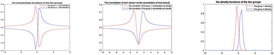
Figure 5.
Fuzzy membership functions, conv-fuzzy-probability densities, and probability densities of two clusters.
4.3. Fuzzy Probability Convolution for the Clustering Task
Following the same principle of probabilistic models presented in Section 2, the proposed clustering method, named Fuzzy Probabilistic Convolution C-Means (FP-Conv-CM), involves estimating the vectors , the common standard deviation , and the membership coefficients, trying to make the realization of the sample of as much as possible in the sense of FP-Conv measure. In this sense, our method involves maximizing the fuzzy probability of the observations:
The parameters must be chosen such that the likelihood is maximum, meaning that the log-likelihood is maximum.
To maximize , we use the partial gradient descent. We present the sample to the fuzzy probability system, and then we set .
At the time , we propose that are known. In addition, thanks to the FP-Conv-CM, we propose that , then we update via the gradient descent method represented by the following equation:
Theorem 1.
We have such that and are the gradients of and , respectively, and is the step of the algorithm following the current direction at time t.
Proof.
We set
Then, we calculate the gradient of the memberships and and we obtain:
and, . Finally, .
Where and □
To update , we use the gradient descent method represented by the following equation:
where is the step of the Algorithm 1 following the current direction at time .
Theorem 2.
We have .
Proof.
In fact, we have
and
then
Then we substitute with
In the following section, we give the version of the proposed system that implements the full-gradient of the loss function:
| Algorithm 1. Fuzzy-Probabilistic-Convolution-C-Means. |
| Requires: Data =, (number of groups), , , m (memberships parameter), b (mini-batch), ITER (maximum number of iterations). |
| Ensure: centers matrix, memberships matrix of to the groups. |
| Initialization: t = 0, , are randomly chosen; For all t = 1, …, ITER Do For all j = 1, …, k Do For all d = 1, …, N Do |
| End For End For End For |
| END |
In this algorithm, the full convolution was approximated by discrete values, which implements a mini-batch of size b: the b-nearest samples of the current sample are used to estimate the continuous convolution.
In the experimentation section, we use the b nearest neighbors of each sample. It is possible to use genetic algorithm to estimate Ω (V)(support of ), Ω such that:
Given a support Ω, it is assumed that there exists an expression for the mathematical expectation of the function of the random variable X, of density of support Ω, resulting from the transfer theorem, based on which . This can be extended to discrete probabilities by summing with a discrete Dirac-like measure. We use Monte Carlo simulation while producing a sample (x1,x2,...,xE) of the random variable X on the support Ω, then we calculate an estimation of based on this sample [54]. Based on the law of large numbers, the empirical mean is a very good estimator. Since the probability densities and membership functions are designed so that they cover, as much as possible, the different data in the set , then the supports of these functions are centered around these data. Thus, it is natural to choose the Monte Carlo samples from these data. In our case, the parameter b is calculated using the formula , where is the number of clusters, because each pair () is supported by the data gained by the group .
5. Experimental Results
5.1. Datasets
To evaluate the performance of FP-Conv-CM, we used six datasets from the UCI [55] repository. Table 1 describes the features of the selected datasets.

Table 1.
Description of the experimental datasets.
5.2. Clustering Results
Table 2 gives the values of Silhouette and Dunn’s indexes obtained by applying FCM, GMM, and FP-Conv-CM to iris, foods, abalone, pima, MAGIC Gamma Telescope, and cloud datasets for a clustering task. Figure 6, Figure 7, Figure 8, Figure 9, Figure 10, Figure 11, Figure 12, Figure 13, Figure 14, Figure 15, Figure 16, Figure 17, Figure 18, Figure 19, Figure 20, Figure 21, Figure 22 and Figure 23 give the silhouettes obtained by applying FCM, GMM, and FP-Conv-CM to these datasets. The forms of these silhouettes show that the groups produced by FCM and FP-Conv-CM are more compact than those produced by GMM. In fact, columns two, four, and six of Table 2 show that FCM and FP-Conv-CM have the largest silhouette values, with those of FP-Conv-CM being slightly higher. However, FP-Conv-CM clearly improves the silhouette of the ones obtained by GMM.
Table 2.
Dunn’s index and Silhouette of FCM, GMM, and FP-Conv-CM on different datasets.
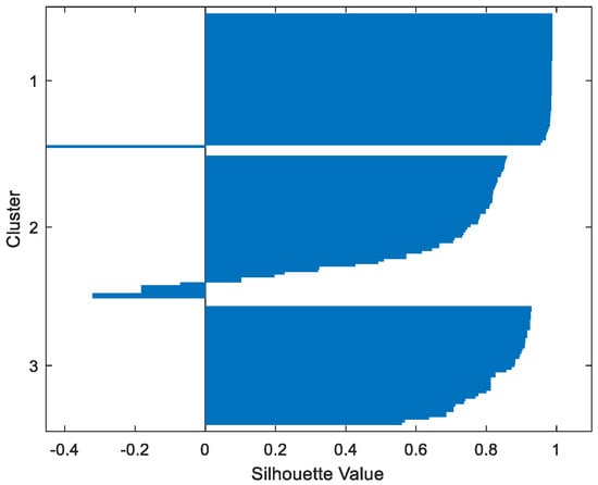
Figure 6.
Iris FP-Conv-CM.
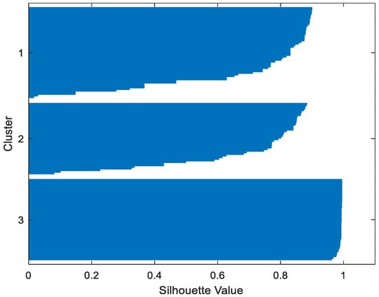
Figure 7.
Iris FCM.
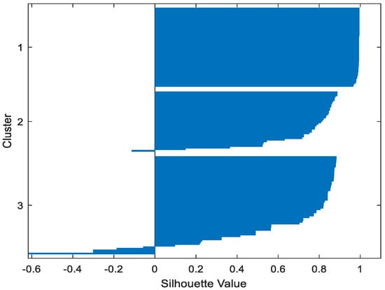
Figure 8.
Iris GMM.
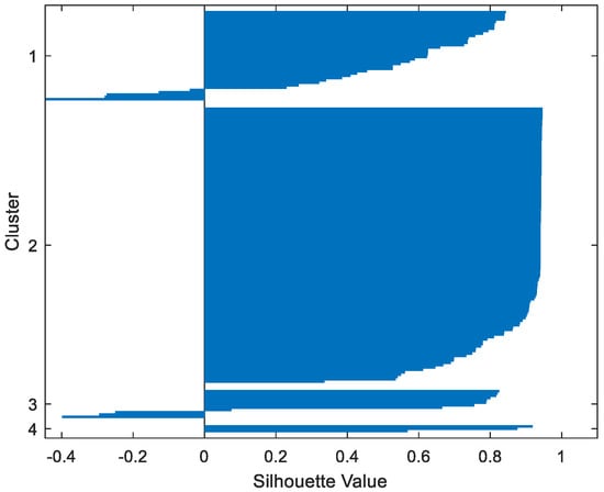
Figure 9.
Foods FP-Conv-CM.
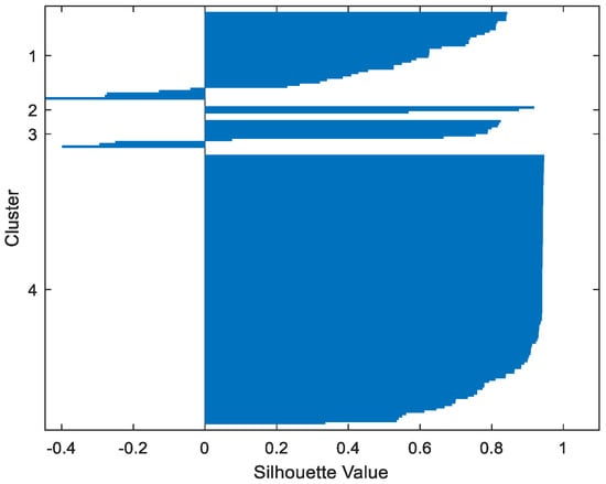
Figure 10.
Foods FCM.
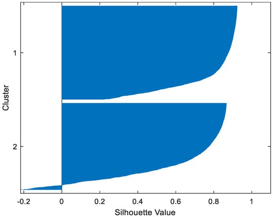
Figure 11.
Foods GMM.
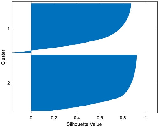
Figure 12.
Abalone FP-Conv-CM.
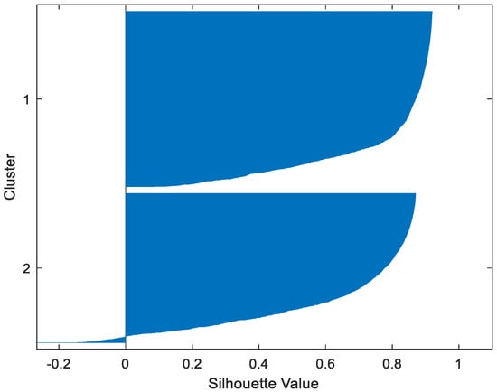
Figure 13.
Abalone FCM.
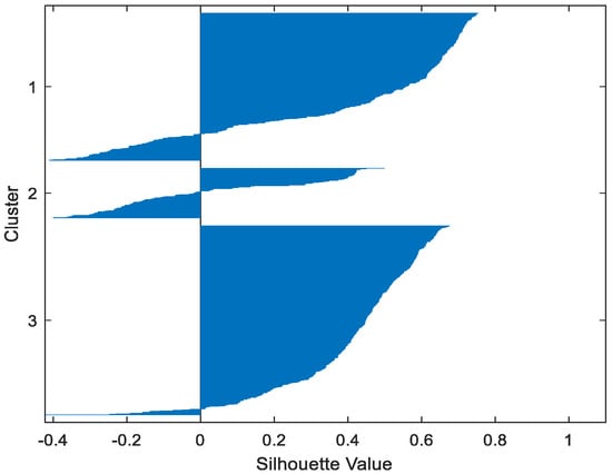
Figure 14.
Abalone GMM.
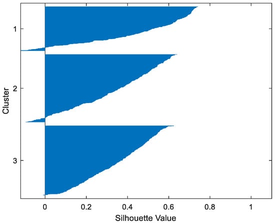
Figure 15.
Pima FP-Conv-CM.
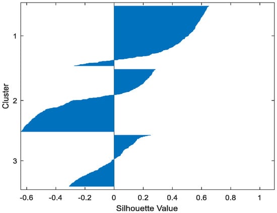
Figure 16.
Pima FCM.
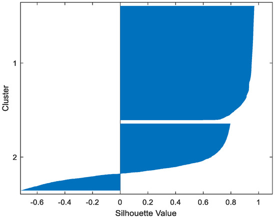
Figure 17.
Pima GMM.
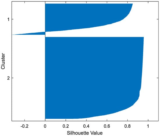
Figure 18.
MAGIC FP-Conv-CM.
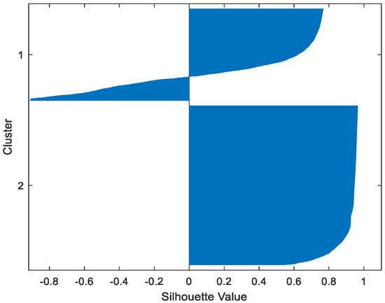
Figure 19.
MAGIC FCM.
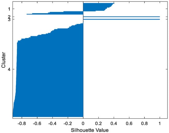
Figure 20.
MAGIC GMM.
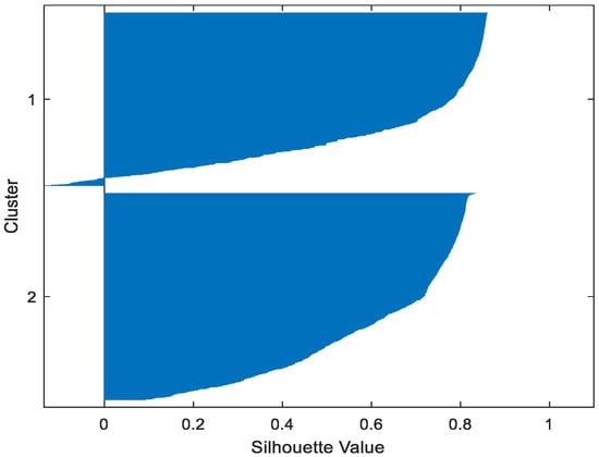
Figure 21.
Cloud FP-Conv-CM.
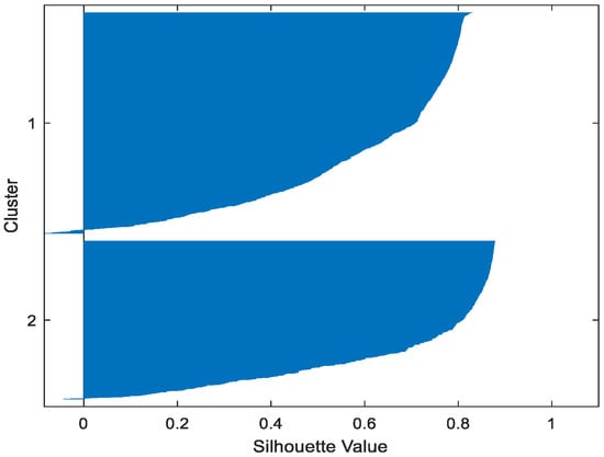
Figure 22.
Cloud FCM.
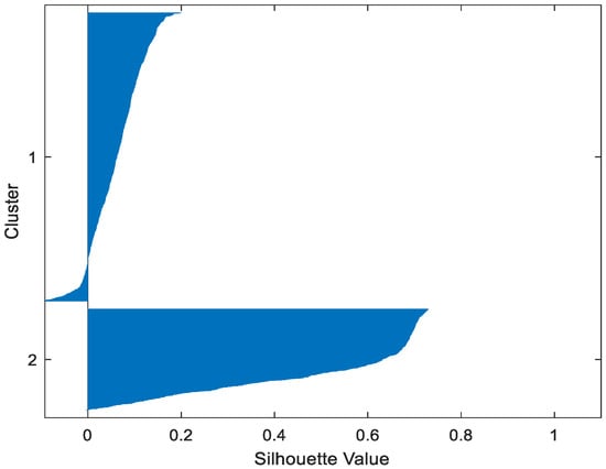
Figure 23.
Cloud GMM.
Considering the six datasets, FCM, GMM, and FP-Conv-CM produce clusters with Dunn’s indexes inferior to 0.065 because of the natural overlapping between different classes of these datasets, which minimizes (the minimal distance between samples in different clusters). In addition, and combining silhouette criterion with Dunn’s index, is very large, especially for FCM and GMM, because some samples are not similar but are assigned to the same groups (see the silhouettes of the groups produced by FCM and GMM using different datasets). However, FP-Conv-CM produces clusters with high Dunn’s values compared with FCM and GMM. This amelioration is achieved thanks to the combination of fuzzy and probabilistic reasonings.
To improve the performance of FP-Conv-CM, we used the attribute selection method named Correlation features Subset Evaluation (CSE) [56]. Table 3 gives Dunn’s index, Silhouette, and CPU time of FP-Conv-CM for different datasets with full and reduced features using the CSE method. Analysis of the six datasets showed that CSE permits the reduction of almost 77% of the attributes in an average CPU time of 3.99 seconds. This resulted in a 24% improvement of the average Silhouette, a 32% improvement of the Dunn’s index, and a 10.7% improvement in CPU time.
Table 3.
Dunn’s index, Silhouette, and CPU time of FP-Conv-CM for different datasets with full and reduced features using the SCE method.
5.3. Image Compression
We evaluated the performance of FP-Conv-CM on an image compression task using several images (see Figure 24, Figure 25 and Figure 26). To avoid cluttering the document with several figures, we give here the results obtained for three images only.

Figure 24.
Archimedes.

Figure 25.
Khwarizmi.
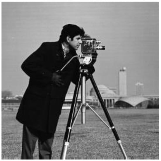
Figure 26.
Cameraman.
5.4. Compression Results
Figure 27, Figure 28, Figure 29, Figure 30, Figure 31, Figure 32, Figure 33, Figure 34 and Figure 35 give the images obtained after decompression of the compression realized using the algorithms based on GMM, FCM, and FP-Conv-CM. Table 4 gives the values of the performance measures MSE, PSNR, and SSIM of different compressions realized with the algorithms that implement GMM, FCM, and FP-Conv-CM.
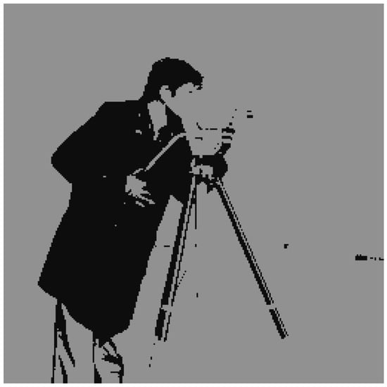
Figure 27.
Cameraman using GMM.
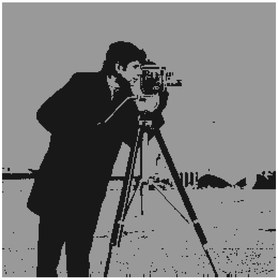
Figure 28.
Cameraman using FCM.
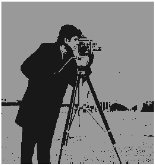
Figure 29.
Cameraman using FP-Conv-CM.
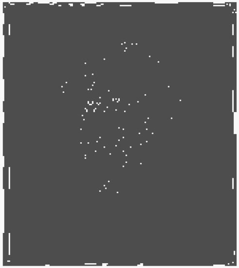
Figure 30.
Archimedes using GMM.

Figure 31.
Archimedes using FCM.

Figure 32.
Archimedes using FP-Conv-CM.
Figure 33.
Khwarizmi using GMM.

Figure 34.
Khwarizmi using FCM.

Figure 35.
Khwarizmi using FP-Conv-CM.
Table 4.
MSE, PEAKSNR, and SSIM values associated with the images compressed by FCM, GMM, and FP-Conv-CM.
Analysis of MSE and PSNR shows that our method permits small improvements in the compression. Analysis of SSIM shows that our method provides an important improvement in compression quality.
6. Conclusions and Future Perspectives
Fuzzy logic makes decisions on the basis of the degree of membership without giving any information about the frequency of events, whereas probability informs us about the frequency of events but gives no information about the degree of membership to a set or class. This paper proposed a convolution fuzzy probabilistic measure that measures the membership degree and the frequency at the same time. Using concrete examples, we proved that the new measure corrects the shortcoming of both the probability measure and the fuzzy logic-based measure. Based on this measure, this paper introduced a new clustering method, named Fuzzy-Probabilistic-Convolution C-Means (FP-Conv-CM). FCM, PKM, and FP-Conv-CM were tested on multiple datasets and compared on the basis of two performance measures: the Silhouette metric and Dunn’s Index. FP-Conv-CM was able to improve the Silhouette value by 1000 and Dunn’s Index by 0.024. In addition, FCM, PKM, and FP-Conv-CM were used for multiple image compressions and were compared based on three performance measures: mean squared error (MSE), peak signal-to-noise ratio (PSNR), and structural similarity index (SSIM). FP-Conv-CM improved MSE by 3000, PSNR by 11, and SSIM by 0.32.
Given the performance of FP-Conv-CM in food grouping, in future we will use it to personalize diets for people with diabetes [57,58]. Also, given the performance of FP-Conv-CM in grouping diabetics, we will use it in the automatic grouping of a population of diabetics to determine the different components of the control models proposed in [59]. Recently, we used GMM and FCM for localization in stochastic environments to improve the results obtained in [60], and we will use FP-Conv-CM to summarize the information from LiDAR sensor, which will overcome the localization limitations caused by both GMM and FCM methods.
Unfortunately, FP-Conv-CM inherits some limitations of classical fuzzy logic, which does not take into account the degree of non-membership to different classes. Moreover, we encountered some difficulties in the selection of an optimal support, and a heuristic method is needed to make a good choice. In future, we will use evolutionary algorithms to choose the patterns that best cover the support of the membership functions and the Gaussians implemented by FC-Conv-CM. In addition, we will introduce the Fuzzy Intuitionist Convolution C-means version to take advantage of the ability of the intuitionist logic to quantify the degree of non-appartenance of patterns to different classes.
Author Contributions
Conceptualization, K.E.M.; Methodology, K.E.M. and V.P.; Software, S.S.; Validation, A.C.; Formal analysis, S.S.; Investigation, K.E.M. and A.C.; Data curation, K.E.M.; Writing—original draft, K.E.M.; Writing—review & editing, V.P., S.S. and A.C.; Supervision, V.P. All authors have read and agreed to the published version of the manuscript.
Funding
This research received no external funding.
Data Availability Statement
Data will only be shared upon request.
Acknowledgments
This work was supported by the Ministry of National Education, Professional Training, Higher Education and Scientific Research (MENFPESRS) and the Digital Development Agency (DDA) of Morocco (Nos. Alkhawarizmi/2020/23).
Conflicts of Interest
The authors declare that they have no conflict of interest.
References
- Rokach, L.; Maimon, O. Clustering methods. In Data Mining and Knowledge Discovery Handbook; Springer: Boston, MA, USA, 2005; pp. 321–352. [Google Scholar] [CrossRef]
- MacQueen, J. Classification and analysis of multivariate observations. In Proceedings of the 5th Berkeley Symposium on Mathematical Statistics and Probability, Berkeley, CA, USA, 1 January 1967; pp. 281–297. [Google Scholar]
- Kriegel, H.P.; Kröger, P.; Sander, J.; Zimek, A. Density-based clustering. Wiley Interdiscip. Rev. Data Min. Knowl. Discov. 2011, 1, 231–240. [Google Scholar] [CrossRef]
- Govaert, G.; Nadif, M. Block clustering with Bernoulli mixture models: Comparison of different approaches. Comput. Stat. Data Anal. 2008, 52, 3233–3245. [Google Scholar] [CrossRef]
- Mirkin, B. Mathematical Classification and Clustering; Springer Science & Business Media: New York, NY, USA, 1996; Volume 11, ISBN 0-7923-4159-7. [Google Scholar]
- Hartuv, E.; Shamir, R. A clustering algorithm based on graph connectivity. Inf. Process. Lett. 2000, 76, 175–181. [Google Scholar] [CrossRef]
- Kohonen, T. Self-organized formation of topologically correct feature maps. Biol. Cybern. 1982, 43, 59–69. [Google Scholar] [CrossRef]
- Venkatkumar, I.A.; Shardaben, S.J.K. Comparative study of data mining clustering algorithms. In Proceedings of the 2016 International Conference on Data Science and Engineering (ICDSE), Cochin, India, 23–25 August 2016; pp. 1–7. [Google Scholar] [CrossRef]
- Rueda, A.; Krishnan, S. Clustering Parkinson’s and age-related voice impairment signal features for unsupervised learning. Adv. Data Sci. Adapt. Anal. 2018, 10, 1840007. [Google Scholar] [CrossRef]
- Mahdavi, M.; Chehreghani, M.H.; Abolhassani, H.; Forsati, R. Novel meta-heuristic algorithms for clustering web documents. Appl. Math. Comput. 2008, 201, 441–451. [Google Scholar] [CrossRef]
- Schubert, E.; Rousseeuw, P.J. Faster k-medoids clustering: Improving the PAM, CLARA, and CLARANS algorithms. In Similarity Search and Applications, Proceedings of the International Conference on Similarity Search and Applications, Newark, NJ, USA, 2–4 October 2019; Springer: Cham, Switzerland, 2019; pp. 171–187. [Google Scholar]
- Samudi, S.; Widodo, S.; Brawijaya, H. The K-Medoids clustering method for learning applications during the COVID-19 pandemic. Sinkron 2020, 5, 116–121. [Google Scholar] [CrossRef]
- Cao, F.; Liang, J.; Li, D.; Bai, L.; Dang, C. A dissimilarity measure for the k-Modes clustering algorithm. Knowl.-Based Syst. 2012, 26, 120–127. [Google Scholar] [CrossRef]
- Oyewole, G.J.; Thopil, G.A. Data clustering: Application and trends. Artif. Intell. Rev. 2022, in press. [Google Scholar] [CrossRef]
- Li, T.; Cai, Y.; Zhang, Y.; Cai, Z.; Liu, X. Deep mutual information subspace clustering network for hyperspectral images. IEEE Geosci. Remote Sens. Lett. 2022, 19, 6009905. [Google Scholar] [CrossRef]
- Zhou, Z.; Dong, X.; Li, Z.; Yu, K.; Ding, C.; Yang, Y. Spatio-temporal feature encoding for traffic accident detection in VANET environment. IEEE Trans. Intell. Transp. Syst. 2022, 23, 19772–19781. [Google Scholar] [CrossRef]
- Kang, Z.; Zhao, X.; Peng, C.; Zhu, H.; Zhou, J.T.; Peng, X.; Chen, W.; Xu, Z. Partition level multiview subspace clustering. Neural Netw. 2020, 122, 279–288. [Google Scholar] [CrossRef]
- Dunn, J.C. A fuzzy relative of the ISODATA process and its use in detecting compactwell-separated clusters. J. Cybern. 1973, 3, 32–57. [Google Scholar] [CrossRef]
- Bezdek, J.C. Pattern Recognition whit Fuzzy Objective Function Algorithms, 2nd ed.; Springer: New York, NY, USA, 1987. [Google Scholar]
- Liao, T.W.; Celmins, A.K.; Hammell, R.J., II. A fuzzy c-means variant for the generation of fuzzy term sets. Fuzzy Sets Syst. 2003, 135, 241–257. [Google Scholar] [CrossRef]
- Krishnapuram, R.; Keller, J.M. A possibilistic approach to clustering. IEEE Trans. Fuzzy Syst. 1993, 1, 98–110. [Google Scholar] [CrossRef]
- Duda, R.O.; Hart, P.E.; Stork, D.G. Pattern Classification and Scene Analysis; Wiley: New York, NY, USA, 1973; Volume 3, pp. 731–739. [Google Scholar]
- Alon, N.; Spencer, J.H. The Probabilistic Method; John Wiley & Sons: Hoboken, NJ, USA, 2016. [Google Scholar]
- Pal, N.R.; Pal, K.; Bezdek, J.C. A mixed c-means clustering model. In Proceedings of the 6th International Fuzzy Systems Conference, Barcelona, Spain, 5 July 1997; Volume 1, pp. 11–21. [Google Scholar]
- Timm, H.; Kruse, R. A modification to improve possibilistic fuzzy cluster analysis. In Proceedings of the 2002 IEEE World Congress on Computational Intelligence, Honolulu, HI, USA, 12–17 May 2002; Volume 2, pp. 1460–1465. [Google Scholar] [CrossRef]
- Timm, H.; Borgelt, C.; Döring, C.; Kruse, R. An extension to possibilistic fuzzy cluster analysis. Fuzzy Sets Syst. 2004, 147, 3–16. [Google Scholar] [CrossRef]
- Zhang, J.S.; Leung, Y.W. Improved possibilistic c-means clustering algorithms. IEEE Trans. Fuzzy Syst. 2004, 12, 209–217. [Google Scholar] [CrossRef]
- Jafar, O.M.; Sivakumar, R. A study on possibilistic and fuzzy possibilistic c-means clustering algorithms for data clustering. In Proceedings of the 2012 International Conference on Emerging Trends in Science, Engineering and Technology (INCOSET), Tamilnadu, India, 13–14 December 2012; pp. 90–95. [Google Scholar] [CrossRef]
- Pal, N.R.; Pal, K.; Keller, J.M.; Bezdek, J.C. A new hybrid c-means clustering model. In Proceedings of the 2004 IEEE International Conference on Fuzzy Systems (IEEE Cat. No. 04CH37542), Budapest, Hungary, 25–29 July 2004; Volume 1, pp. 179–184. [Google Scholar] [CrossRef]
- Pal, N.R.; Pal, K.; Keller, J.M.; Bezdek, J.C. A possibilistic fuzzy c-means clustering algorithm. IEEE Trans. Fuzzy Syst. 2005, 13, 517–530. [Google Scholar] [CrossRef]
- Azzouzi, S.; El-Mekkaoui, J.; Hjouji, A.; El Khalfi, A. An effective modified possibilistic Fuzzy C-Means clustering algorithm for noisy data problems. In Proceedings of the 2021 Fifth International Conference on Intelligent Computing in Data Sciences (ICDS), Fez, Morocco, 20–22 October 2021; pp. 1–7. [Google Scholar] [CrossRef]
- Guo, Y.; Sengur, A. NCM: Neutrosophic c-means clustering algorithm. Pattern Recognit. 2015, 48, 2710–2724. [Google Scholar] [CrossRef]
- Guo, Y.; Sengur, A. NECM: Neutrosophic evidential c-means clustering algorithm. Neural Comput. Appl. 2015, 26, 561–571. [Google Scholar] [CrossRef]
- Akbulut, Y.; Şengür, A.; Guo, Y.; Polat, K. KNCM: Kernel neutrosophic c-means clustering. Appl. Soft Comput. 2017, 52, 714–724. [Google Scholar] [CrossRef]
- Chiang, J.H.; Hao, P.Y. A new kernel-based fuzzy clustering approach: Support vector clustering with cell growing. IEEE Trans. Fuzzy Syst. 2003, 11, 518–527. [Google Scholar] [CrossRef]
- Graves, D.; Pedrycz, W. Kernel-based fuzzy clustering and fuzzy clustering: A comparative experimental study. Fuzzy Sets Syst. 2010, 161, 522–543. [Google Scholar] [CrossRef]
- Huang, H.C.; Chuang, Y.Y.; Chen, C.S. Multiple kernel fuzzy clustering. IEEE Trans. Fuzzy Syst. 2011, 20, 120–134. [Google Scholar] [CrossRef]
- Chen, L.; Chen, C.P.; Lu, M. A multiple-kernel fuzzy c-means algorithm for image segmentation. IEEE Trans. Syst. Man Cybern. Part B 2011, 41, 1263–1274. [Google Scholar] [CrossRef] [PubMed]
- Crespo, F.; Weber, R. A methodology for dynamic data mining based on fuzzy clustering. Fuzzy Sets Syst. 2005, 150, 267–284. [Google Scholar] [CrossRef]
- Munusamy, S.; Murugesan, P. Modified dynamic fuzzy c-means clustering algorithm–application in dynamic customer segmentation. Appl. Intell. 2020, 50, 1922–1942. [Google Scholar] [CrossRef]
- Ruspini, E.H.; Bezdek, J.C.; Keller, J.M. Fuzzy clustering: A historical perspective. IEEE Comput. Intell. Mag. 2019, 14, 45–55. [Google Scholar] [CrossRef]
- El Moutaouakil, K.; Touhafi, A. A New Recurrent Neural Network Fuzzy Mean Square Clustering Method. In Proceedings of the 2020 5th International Conference on Cloud Computing and Artificial Intelligence: Technologies and Applications (CloudTech), Marrakesh, Morocco, 28–30 May 2020; pp. 1–5. [Google Scholar] [CrossRef]
- El Moutaouakil, K.; Yahyaouy, A.; Chellak, S.; Baizri, H. An Optimized Gradient Dynamic-Neuro-Weighted-Fuzzy Clustering Method: Application in the Nutrition Field. Int. J. Fuzzy Syst. 2022, 24, 3731–3744. [Google Scholar] [CrossRef]
- El Moutaouakil, K.; El Ouissari, A.; Hicham, B.; Saliha, C.; Cheggour, M. Multi-objectives optimization and convolution fuzzy C-means: Control of diabetic population dynamic. RAIRO-Oper. Res. 2022, 56, 3245–3256. [Google Scholar] [CrossRef]
- Saberi, H.; Sharbati, R.; Farzanegan, B. A gradient ascent algorithm based on possibilistic fuzzy C-Means for clustering noisy data. Expert Syst. Appl. 2021, 191, 116153. [Google Scholar] [CrossRef]
- Surono, S.; Putri, R.D.A. Optimization of Fuzzy C-Means Clustering Algorithm with Combination of Minkowski and Chebyshev Distance Using Principal Component Analysis. Int. J. Fuzzy Syst. 2021, 23, 139–144. [Google Scholar] [CrossRef]
- Xu, W.; Xu, Y. An improved index for clustering validation based on Silhouette index and Calinski-Harabasz index. IOP Conf. Ser. Mater. Sci. Eng. 2019, 569, 052024. [Google Scholar]
- Pérez-Ortega, J.; Roblero-Aguilar, S.S.; Almanza-Ortega, N.N.; Frausto Solís, J.; Zavala-Díaz, C.; Hernández, Y.; Landero-Nájera, V. Hybrid Fuzzy C-Means Clustering Algorithm Oriented to Big Data Realms. Axioms 2022, 11, 377. [Google Scholar] [CrossRef]
- Gu, Y.; Ni, T.; Jiang, Y. Deep Possibilistic C-means Clustering Algorithm on Medical Datasets. Comput. Math. Methods Med. 2022, 2022, 3469979. [Google Scholar] [CrossRef] [PubMed]
- Inaba, M.; Katoh, N.; Imai, H. Applications of weighted Voronoi diagrams and randomization to variance-based k-clustering. In Proceedings of the Tenth Annual Symposium on Computational Geometry, New York, NY, USA, 6–8 June 1994; pp. 332–339. [Google Scholar]
- Wang, Z.; Simoncelli, E.P.; Bovik, A.C. Multiscale structural similarity for image quality assessment. In Proceedings of the Conference Record of the Thirty-Seventh Asilomar Conference on Signals, Systems and Computers, California, CA, USA, 9–12 November 2003; Volume 2, pp. 1398–1402. [Google Scholar]
- Hartigan, J.A.; Wong, M.A. Algorithm AS 136: A k-means clustering algorithm. J. R. Stat. Soc. Ser. C 1979, 28, 100–108. [Google Scholar] [CrossRef]
- Bezdek, J.C. Pattern Recognition with Fuzzy Objective Function Algorithms; Springer Science & Business Media: New York, NY, USA, 2013. [Google Scholar]
- Ngomo, M.; Kimbonguila, A. Caracterisation des agglomerats des fines particules par combinaison des techniques numeriques de la geometrie algorithmique et la methode de monte-carlo: Determination de la morphologie, de la compacite et de la porosite. Ann. Sci. Tech. 2022, 21, 1–18. [Google Scholar]
- Machine Learning Repository UCI. Available online: http://archive.ics.uci.edu/ml/datasets.html (accessed on 10 January 2022).
- Hancer, E.; Bing, X.; Mengjie, Z. Differential evolution for filter feature selection based on information theory and feature ranking. Knowl.-Based Syst. 2018, 140, 103–119. [Google Scholar] [CrossRef]
- Ahourag, A.; Chellak, S.; Cheggour, M.; Baizri, H.; Bahri, A. Quadratic Programming and Triangular Numbers Ranking to an Optimal Moroccan Diet with Minimal Glycemic Load. Stat. Optim. Inf. Comput. 2023, 11, 85–94. [Google Scholar]
- El Moutaouakil, K.; Baizri, H.; Chellak, S. Optimal fuzzy deep daily nutrients requirements representation: Application to optimal Morocco diet problem. Math. Model. Comput. 2022, 9, 607–615. [Google Scholar] [CrossRef]
- Abdellatif, E.O.; Karim, E.M.; Saliha, C.; Hicham, B. Genetic algorithms for optimal control of a continuous model of a diabetic population. In Proceedings of the 2022 IEEE 3rd International Conference on Electronics, Control, Optimization and Computer Science (ICECOCS), Kenitra, Morocco, 1–2 December 2022. [Google Scholar]
- Charroud, A.; El Moutaouakil, K.; Palade, V.; Yahyaouy, A. XDLL: Explained Deep Learning LiDAR-Based Localization and Mapping Method for Self-Driving Vehicles. Electronics 2023, 12, 567. [Google Scholar] [CrossRef]
Disclaimer/Publisher’s Note: The statements, opinions and data contained in all publications are solely those of the individual author(s) and contributor(s) and not of MDPI and/or the editor(s). MDPI and/or the editor(s) disclaim responsibility for any injury to people or property resulting from any ideas, methods, instructions or products referred to in the content. |
© 2023 by the authors. Licensee MDPI, Basel, Switzerland. This article is an open access article distributed under the terms and conditions of the Creative Commons Attribution (CC BY) license (https://creativecommons.org/licenses/by/4.0/).