Redesigning Embedding Layers for Queries, Keys, and Values in Cross-Covariance Image Transformers

Abstract

There are several attempts in vision transformers to reduce quadratic time complexity to linear time complexity according to increases in the number of tokens. Cross-covariance image transformers (XCiT) are also one of the techniques utilized to address the issue. However, despite these efforts, the increase in token dimensions still results in quadratic growth in time complexity, and the dimension is a key parameter for achieving superior generalization performance. In this paper, a novel method is proposed to improve the generalization performances of XCiT models without increasing token dimensions. We redesigned the embedding layers of queries, keys, and values, such as separate non-linear embedding (SNE), partially-shared non-linear embedding (P-SNE), and fully-shared non-linear embedding (F-SNE). Finally, a proposed structure with different model size settings achieved $71.4\%,77.8\%$, and $82.1\%$ on ImageNet-1k compared with $69.9\%,77.1\%$, and $82.0\%$ acquired by the original XCiT models, namely XCiT-N12, XCiT-T12, and XCiT-S12, respectively. Additionally, the proposed model achieved $94.8\%$ in transfer learning experiments, on average, for CIFAR-10, CIFAR-100, Stanford Cars, and STL-10, which is superior to the baseline model of XCiT-S12 ($94.5\%$). In particular, the proposed models demonstrated considerable improvements on the out-of-distribution detection task compared to the original XCiT models.

1. Introduction

Transformer models have attracted considerable research attention as dominant models in deep learning because of their superior performances [1,2]. Transformers were first used in natural language processing (NLP) [1] and are subsequently being widely used as the backbone network for state-of-the-art models [3,4,5]. Recently, transformers have also been used in the computer vision field. Vision transformers (ViT) [6] exhibit superior generalization performances to that of traditional convolutional neural network (CNN) architectures [6,7,8].

In standard vision transformers, tokens, which are sequences of cropped image patches extracted from two-dimensional color images, are used. Then, a global self-attention mechanism is applied to extract the relationship among tokens. This procedure can be used to extract information on the long-range relationship among tokens, in contrast to CNNs, in which the local relationship of image pixels is considered. However, this process requires extensive computations that increase quadratically with image resolution [6,9]. To alleviate these inefficiencies, convolutional features have been added explicitly in transformers [10,11,12,13]. Another attempt is cross-covariance image transformers (XCiT) [9], which utilize a modified multi-head self-attention (MHSA) technique based on a transposed self-attention mechanism. XCiT considerably reduced time complexity from $O\left(N^{2}d\right)$ to $O\left(N{d}^2\right)$, where N is the number of tokens and d is the dimension of each token. This implies that the number of tokens is more crucial than the dimension of each token. However, increasing d is also harmful in terms of computational cost (see the original XCiT paper [9]. The XCiT-N12 and XCiT-T12 models in

Table 1. Corresponding output dimensions of Q, K, and V embedding layers to each model variant are listed below.

Model	Small (S)		Medium (M)		Large (L)
	d	${\mathit{d}}_{\mathit{q},\mathit{k},\mathit{v}}$	d	${\mathit{d}}_{\mathit{q},\mathit{k},\mathit{v}}$	d	${\mathit{d}}_{\mathit{q},\mathit{k},\mathit{v}}$
SNE	128	64	192	96	384	192
P-SNE	128	96	192	144	384	288
F-SNE-C	128	128	192	192	384	384
F-SNE-C8*	128	186	192	282	384	556
F-SNE-C16*	128	182	192	276	384	544

of the paper have different d, and the other hyperparameters are identical. GFLOPs for each model do not linearly increase with d. The computational concern of increasing d is not more dominant than N but is also problematic.), and research on resolving the issue is required. To the best of our knowledge, no study has focused on resolving this problem.

To resolve this problem, a novel efficient architecture might be developed to ensure linear time complexities in both N and d. In the second method of resolving the problem, the performances of the conventional vision transformer models with small d are maximized. In this paper, instead of presenting a new, efficient architecture design, we try to maximize generalization performances by redesigning the embedding layers for queries (Q), keys (K), and values (V) with fixed d values, which are the same values as in the original XCiT models. We speculate that improved embedding spaces may exist under a fixed dimension of space.

To achieve the goal, we propose three repetitive structures in XCiT models. The structures are simple and can effectively increase generalization performances in XCiT models. First, a two-layer embedding structure with a rectified linear unit activation function (ReLU) is proposed. This method is called a separate non-linear embedding (SNE) method. In contrast to the original embedding in XCiT models, the structure can transform the input data into a non-linear space with activation functions. The second structure is a one-layer shared structure, which is a variant of the first structure. This method is the partially shared non-linear embedding (P-SNE) method. The third structure is a two-layer shared structure with trainable code parameters that can improve the original self-attention mechanism used in conventional transformers. This structure is a fully shared non-linear embedding (F-SNE) model.

Finally, experimental results demonstrate that the proposed method outperforms the original XCiT models in the ImageNet [14] classification task and transfer learning on multiple datasets (i.e., CIFAR-10, CIFAR-100 [15], Stanford Cars [16], and STL-10 [17]). Furthermore, the proposed method outperforms the original XCiT models in the out-of-distribution (OOD) detection task. The contributions of this paper can be summarized as follows:

• We show that two simple and well-known structures, SNE and P-SNE, can improve the generalization ability of XCiT models under the small value of d.
• A novel structure called F-SNE was proposed, which outperforms the original XCiT, SNE, and P-SNE models. The structure is a fully shared model, and a code was adopted to feed different input values to the layers.
• The original XCiT models could not approach the top record among state-of-the-art (SOTA) transformer models in image classification tasks, but the modified XCiT models with the proposed structures are comparable with current SOTA models, such as the Swin [18], CeiT [19], and ViTAE [20] models.
• The high uncertainty prediction capability of the proposed structure, F-SNE, which largely improved the performance of the OOD detection task, was validated.

2. Related Works

We first summarize related works in transformer models as three aspects of architecture, computational cost, and designing embedding layers.

2.1. Architectures

When ViT was first proposed, global self-attention was applied among image tokens to handle long-range information [6]. However, global self-attention requires large-scale pre-training, and its computation quadratically increases according to the input size [8,21]. To address this problem, ViTAE [20], ConViT [22], and LocalViT [23] proposed the use of convolutions besides self-attention to embed both local and global features into the transformer, and T2T-ViT [11] progressively restructured image tokens into reduced-length tokens including local features. Furthermore, Swin transformer [18] utilized windowed attention with a hierarchical architecture to efficiently improve performance.

Few additional approaches to designing embedding layers have been proposed to embed better features in the tokens without increasing dimensionality. CvT [10] utilized convolutional projection for the Q, K, and V embedding of the transformer encoder to take advantage of both the CNN and transformer. In the case of ViP [24], learnable part representations are shared across transformer blocks to make Q, K, or V embeddings. However, linear projection was used to make those embeddings. There are no studies that use fully shared models, such as the proposed F-SNE structure. However, conventional self-attention with linearly projected Q, K, and V embeddings may not sufficiently handle this concern.

2.2. Approaches for Efficient Computational Cost

Current studies on vision transformers mainly focus on not only applying inductive bias to vision transformers but also reducing the computational complexity from quadratic to linear, such as GFNet [25], AFNO [26], and XCiT [9]. These approaches usually have proposed efficient self-attention mechanisms or replaced self-attention with another global operation, such as Fourier transformation. XCiT [9] is one of the representative approaches that focuses on reducing the computational complexity. It introduces cross-covariance attention (XCA) instead of standard self-attention. XCA effectively reduces computation without a large performance gap compared to the baseline. However, XCA has a limitation in that the computation quadratically increases according to the dimensionality of the tokens, which motivates us to find better token embeddings while maintaining dimensionality. However, it does not consider $Q,K$, and V embedding, which directly affects the attention operation. In contrast to these works, we introduce $Q,K$, and V embedding techniques to improve the performance of image recognition.

3. Attention Mechanism in Vision Transformer

In this section, we introduce preliminary knowledge about the self-attention and cross-covariance attention mechanisms in vision transformers.

3.1. Self-Attention

Conventional transformers adopt self-attention as the core operation of the network [1,6,27]. In the transformer, the input token X is projected by the linear projection layer $W_q$, $W_k$, and $W_v$ to embed Q, K, and V vectors, respectively. Then, the self-attention is operated as follows:

$$\begin{array}{c}\hfill SA(Q,K,V)=Softmax\left(\frac{Q{K}^T}{\sqrt{d_k}}\right)V,\end{array}$$

(1)

where $SA(Q,K,V)$ is the output of self-attention, and Q, K, and V are processed by the following linear projection:

$$\begin{array}{c}\hfill \begin{array}{c}\hfill Q=X{W}_q,K=X{W}_k,V=X{W}_v,\end{array}\end{array}$$

(2)

on $X\in R^{N\times d}$, $W_q\in R^{d\times d_q}$, $W_k\in R^{d\times d_k}$, $W_v\in R^{d\times d_v}$, where N is the number of tokens and d is the token dimension. This process is typically conducted in a multi-headed manner. When the number of heads is h, $d_q=d_k=d_v=d/h$.

3.2. Cross-Covariance Attention

Cross-covariance attention is a modified self-attention mechanism that can reduce the computational complexity from $O\left(N^{2}d\right)$ to $O\left(N{d}^2\right)$ [9,28]. XCiT [9] proposed the use of cross-covariance attention instead of standard self-attention, which is widely used in transformer networks, demonstrating its SOTA performance in CV tasks, including in, for example, ImageNet classification, self-supervised learning, and semantic segmentation. They conducted feature dimension self-attention instead of token dimension self-attention, which is used in the standard transformer encoder. By simply transposing Q, K, and V and reversing the order of the dot product, the computational complexity was reduced from quadratic to linear with the number of tokens, N. This transposed feature dimension self-attention can be represented as follows:

$$\begin{array}{c}\hfill XCA(Q,K,V)=V·Softmax\left(\frac{{\widehat{K}}^T\widehat{Q}}{\tau }\right),\end{array}$$

(3)

where $XCA(Q,K,V)$ is the output of cross-covariance attention and $\widehat{Q}$, $\widehat{K}$, and $\tau$ are the $l2$-normalized Q, K vector, and temperature scaling parameter, respectively. This provides better generalization performances than a traditional self-attention mechanism, and XCiT was adopted as a baseline model to verify the performance of the proposed method.

4. Method

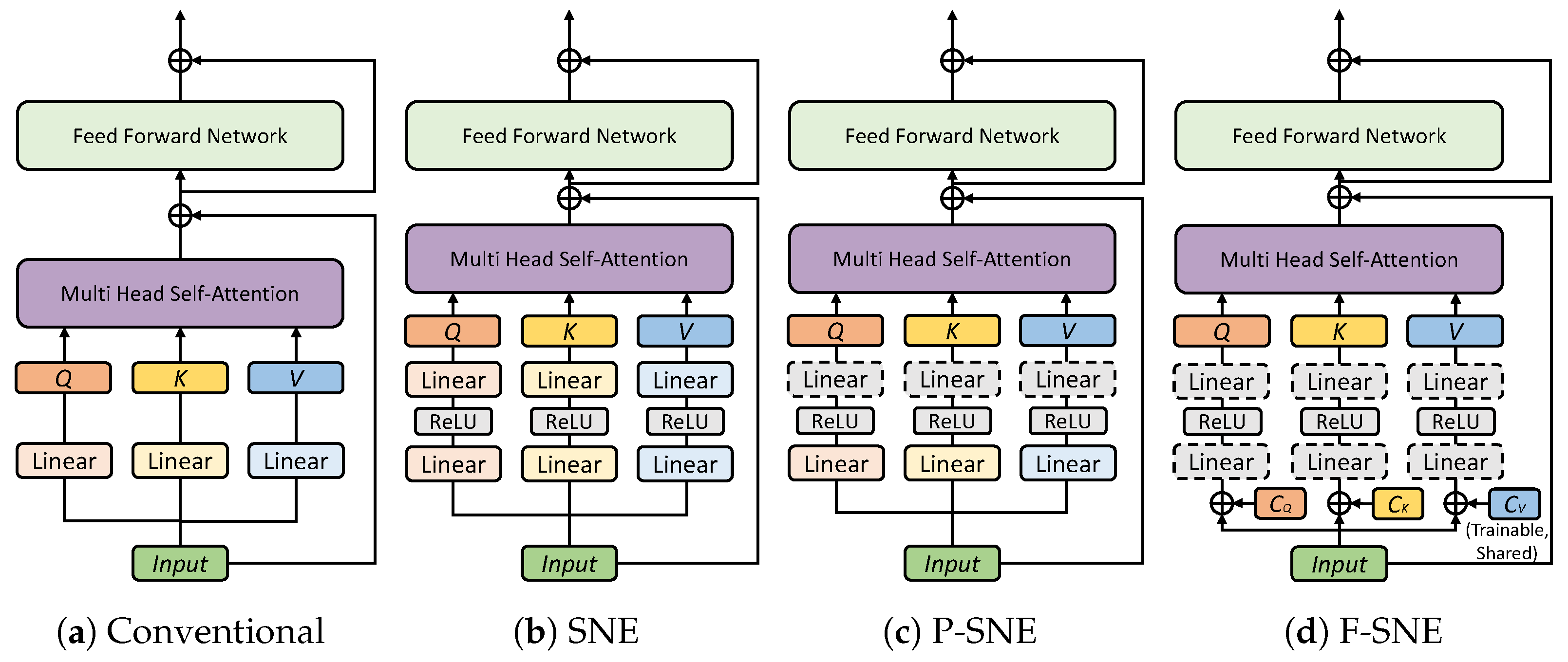
As mentioned in Equation (2), in the conventional embedding method, a linear layer was used for each Q, K, and V. The layer is not shared across the embedding spaces of Q, K, and V. We propose three types of embedding techniques to improve the performance of XCiT, as displayed in Figure 1.

4.1. Separate Non-Linear Embedding

In contrast to the original XCiT-based models, non-linear transformations were applied to extract Q, K, and V, as follows:

$$\begin{array}{c}\hfill \begin{array}{c}\hfill Q=\sigma \left(X{W}_q^{\left(1\right)}\right)W_q^{\left(2\right)},\\ \hfill K=\sigma \left(X{W}_k^{\left(1\right)}\right)W_k^{\left(2\right)},\\ \hfill V=\sigma \left(X{W}_v^{\left(1\right)}\right)W_v^{\left(2\right)},\end{array}\end{array}$$

(4)

where $W_q^{\left(1\right)}\in R^{d\times d_q}$ and $W_q^{\left(2\right)}\in R^{d_q\times d}$ represent the weight parameters of the first and second fully connected layers, respectively, and the layers encode the input token as Q. $W_k^{\left(1\right)}\in R^{d\times d_k}$ and $W_k^{\left(2\right)}\in R^{d_k\times d}$ correspond to K, and $W_v^{\left(1\right)}\in R^{d\times d_v}$ and $W_v^{\left(2\right)}\in R^{d_v\times d}$ extract V. $\sigma$ is an activation function. Based on the obtained Q, K, and V, Equation (3) is computed for self-attention.

The layers for the SNE consist of two fully connected layers with an activation function (e.g., ReLU) to conduct a non-linear transformation of input tokens. The non-linear embedding approach exhibits the following advantages. This method could increase the total number of non-linearities of the model. Under a limited number of parameters, the increased number of non-linearities could positively affect generalization. Furthermore, the search space can be expanded to find new combinations of Q, K, and V in non-linear embedding spaces.

4.2. Partially Shared Non-Linear Embedding

P-SNE shares a layer from two fully connected layers in the SNE model. There are two options for which the layer will be selected (i.e., first or second layers). Sharing the first layer is similar to the linear embedding originally used in the XCiT model. The shared first layer produces the same output because the input values are the same. Consequently, we chose the second layer to be shared among Q, K, and V. The shared second layer linearly transforms each activation value extracted from the first non-linear layer. With the shared layer, Q, K, and V can share knowledge on how to build each token.

In general, separate layers of original or SNE structures could result in a problem. In separate layers, even if one of the layers responsible for Q, K, and V extraction does not learn well, the training loss can be minimized. Thus, the network is trained well even if one of the three separate layers for Q, K, and V is not properly updated. However, the phenomenon cannot be shown in the shared layers.

Finally, Q, K, and V in the P-SNE are extracted as follows:

$$\begin{array}{c}\hfill \begin{array}{c}\hfill Q=\sigma \left(X{W}_q^{\left(1\right)}\right)W_s^{\left(2\right)},\\ \hfill K=\sigma \left(X{W}_k^{\left(1\right)}\right)W_s^{\left(2\right)},\\ \hfill V=\sigma \left(X{W}_v^{\left(1\right)}\right)W_s^{\left(2\right)},\end{array}\end{array}$$

(5)

where $W_s^{\left(2\right)}\in R^{d_s\times d}$ denotes the weight parameters of the shared second layer when $d_s=d_q=d_k=d_v$. The weight parameters $W_q^{\left(2\right)}$, $W_k^{\left(2\right)}$, and $W_v^{\left(2\right)}$ of the second layer of the SNE were replaced with $W_s^{\left(2\right)}$.

4.3. Fully Shared Non-Linear Embedding

For F-SNE, we first integrate the Q, K, and V projection layers $W_q^{\left(i\right)}$, $W_k^{\left(i\right)}$, and $W_v^{\left(i\right)}$ into the shared projection layers $W_s^{\left(i\right)}$ for $i=\{1,2\}$, as shown in Figure 1d. Instead of Q, K, and V projection layers that separately transform input token X into Q, K, and V vectors, the shared projection layers transform the input token X into Q, K, and V in the same embedding space.

When fully shared projection layers are used, we adopt codes of $C_q$, $C_k$, and $C_v$. The codes correspond to Q, K, and V embeddings and convert the same inputs into three different vectors. $C_q$, $C_k$, and $C_v$ are trainable vectors that are concatenated to the input token X before passing the shared projection layers $W_s$. Additionally, the same $C_q$, $C_k$, and $C_v$ are shared among all the encoders in the transformer. By this sharing, codes converge at the optimal semantic representation of Q, K, and V that exists consistently regardless of the encoder.

Finally, Q, K, and V embeddings by the proposed shared projection layers with codes $C_q$, $C_k$, and $C_v$ can be represented as follows:

$$\begin{array}{c}\hfill \begin{array}{c}\hfill Q=\sigma \left((X\oplus C_q)W_s^{\left(1\right)}\right)W_s^{\left(2\right)},\\ \hfill K=\sigma \left((X\oplus C_k)W_s^{\left(1\right)}\right)W_s^{\left(2\right)},\\ \hfill V=\sigma \left((X\oplus C_v)W_s^{\left(1\right)}\right)W_s^{\left(2\right)},\end{array}\end{array}$$

(6)

on $X\in R^{N\times d}$ and $C_q$, $C_k$, $C_v\in R^{N\times c}$, where ⊕ denotes vector concatenation and c is an arbitrary code size. Here, $C_q$, $C_k$, $C_v\in R^{1\times c}$, but these are repeated N times to match the dimension with X. Codes $C_q$, $C_k$, and $C_v$ are concurrently computed with the network parameter $\theta$ to minimize the loss function as follows:

$$\widehat{\theta },{\widehat{C}}_q,{\widehat{C}}_k,{\widehat{C}}_v=\underset{\theta ,C_q,C_k,C_v}{min}\mathcal{L}(D;\theta ,C_q,C_k,C_v)$$

(7)

where $\mathcal{L}$ is a loss function (e.g., cross-entropy loss). D is the training dataset, and $\theta$ denotes the network parameters of the transformer network, including the embedding layers of Q, K, and V (i.e., $W_q,W_k,W_v$, or $W_s$). Note that $C_q$, $C_k$, $C_v$, and $\theta$ are updated at the same step. A detailed procedure of Equation (7) is implemented as Algorithm 1.

Algorithm 1 F-SNE

Require:  D: Training data, $\theta$: Network parameters  1: Randomly initialize $\theta ,C_q,C_k,C_v$  2: while not done do  3:     Sample batch of data D  4:     Compute $\mathcal{L}(D;\theta ,C_q,C_k,C_v)$ in Equation (7)  5:     Update $\theta ,C_q,C_k,C_v$  6: end while

5. Experiments and Results

We first introduce the detailed experimental setup and datasets. Then, we evaluate the ImageNet-1k classification performance of the proposed structures according to their scale and conduct brief experiments using distillation. Additionally, we use those models to transfer to the other datasets (i.e., CIFAR-10, CIFAR-100, Stanford Cars, and STL-10). Lastly, we evaluate uncertainty prediction performance through the OOD detection task.

5.1. Experimental Setup

Experiments for the proposed methods were conducted based on XCiT models. In the following sections, the notations XCiT-N12, XCiT-T12, and XCiT-S12 were used to denote XCiT-Nano, XCiT-Tiny, and XCiT-Small models with 12 blocks. We implemented small (S), medium (M), large (L) models based on XCiT-N12, XCiT-T12, and XCiT-S12, respectively. The input image size of the models was fixed at 224 × 224. The models were trained using a batch size of 4096, 2816, and 1280 for XCiT-N12, XCiT-T12, and XCiT-S12-based models, respectively. For ImageNet training, we trained the model for 400 epochs with an initial learning rate of $5\times {10}^{-4}$. For transfer learning, an initial learning rate of $5\times {10}^{-5}$ was used for 1000 epochs of training. We followed other experimental setups of the XCiT. Overall experiments were conducted on NVIDIA DGX A100 (8 GPUs).

For the Q, K, and V projection layers, dimensions of output tokens depicted in Table 1 were used according to the variants. The starred (*) model is used to compare the proposed method using the same number of parameters as the original XCiT model. Additionally, the shared layers for the F-SNE-Cn-S, F-SNE-Cn-M, and F-SNE-Cn-L models have input dimensions of $(128+n)$, $(192+n)$, and $(384+n)$ to take the input concatenated with the n-dimensional code. Code is a vector of arbitrary code size (e.g., $n=8,16,32,64$) defined outside the encoder to be shared among encoders. For a fair comparison, we compare the number of parameters and image size as well as the performance in the following sections. In the case of F-SNE, codes were also included in the number of model parameters.

5.2. Dataset

We used ImageNet-1k [14] to train the models from scratch. Then, we used the CIFAR-10, CIFAR-100 [15], Stanford Cars [16], and STL-10 [17] datasets to evaluate transfer learning performance. In the case of an out-of-distribution (OOD) detection task, we used the CIFAR-10 dataset as an in-distribution (ID) and the LSUN-R, LSUN-C [29], iSUN [30], SVHN [31], and DTD [32] datasets as OOD. The detailed information of these datasets is described below.

The ImageNet dataset consists of 1.28 M training images and 50,000 validation images with 1000 categories.

The CIFAR-10 and CIFAR-100 datasets consist of 50,000 training images and 10,000 test images with 10 and 100 categories, respectively.

The Stanford Cars dataset consists of 8144 training images and 8041 test images of 196 categories.

The STL-10 dataset contains 5000 training images and 8000 test images from 10 categories.

The LSUN dataset consists of 10 scene classes and contains around 120,000 to 3,000,000 images for each class. It has 1000 test images for each class. LSUN-R (resize) and LSUN-C (crop) were reconstructed by [33] for OOD detection, so we used these datasets.

The iSUN dataset consists of 6000 training images, 926 validation images, and 2000 test images. We used whole images from this dataset for OOD detection.

The SVHN dataset consists of 73,257 training images and 26,032 test images from 10 digit classes. We randomly selected 10,000 images from test images while uniformly sampling for 10 classes when evaluating OOD detection.

The DTD dataset consists of 5640 texture images from 47 classes. We used whole images of this dataset for OOD detection.

5.3. Imagenet Classification

Table 2. Proposed models were evaluated on ImageNet classification task. The number of parameters was constrained to be below 4 M to be compared to the small (S) models.

Model	Image Size	Param #	Top-1 (%)
Mobile-Former-26M	$224\times 224$	3.2 M	64.0
Mobile-Former-52M	$224\times 224$	3.5 M	68.7
XCiT-N12 (baseline)	$224\times 224$	3.1M	69.9
F-SNE-C16-S (ours)	$224\times 224$	2.9 M	70.2
PVTv2-B0	$224\times 224$	3.4 M	70.5
F-SNE-C8-S (ours)	$224\times 224$	2.9 M	70.6
F-SNE-C16*-S (ours)	$224\times 224$	3.1 M	70.6
F-SNE-C8*-S (ours)	$224\times 224$	3.1 M	70.8
SNE-S (ours)	$224\times 224$	3.1 M	70.9
P-SNE-S (ours)	$224\times 224$	3.1 M	71.4

,

Table 3. Proposed models were evaluated on ImageNet classification task. The number of parameters was constrained to be below 10 M to be compared to the medium (M) models.

Model	Image Size	Param #	Top-1 (%)
ViT-Ti	$224\times 224$	5.7 M	68.7
T2T-ViT-7	$224\times 224$	4.3 M	71.7
DeiT-Ti	$224\times 224$	5.7 M	72.2
LocalViT-T2T	$224\times 224$	4.3 M	72.5
Mobile-Former-96M	$224\times 224$	4.6 M	72.8
PiT-Ti	$224\times 224$	4.9 M	73.0
ConViT-Ti	$224\times 224$	5.7 M	73.1
GFNet-Ti	$224\times 224$	7 M	74.6
LocalViT-T	$224\times 224$	5.9 M	74.8
ConT-Ti	$224\times 224$	5.8 M	74.9
ViP-Mo	$224\times 224$	5.3 M	75.1
ViTAE-T	$224\times 224$	4.8 M	75.3
CeiT-T	$224\times 224$	6.4 M	76.4
ConT-S	$224\times 224$	10.1 M	76.5
T2T-ViT-12	$224\times 224$	6.9 M	76.5
F-SNE-C8-M (ours)	$224\times 224$	6.3 M	76.8
XCiT-T12 (baseline)	$224\times 224$	6.7 M	77.1
F-SNE-C16-M (ours)	$224\times 224$	6.3 M	77.2
ResT-Lite	$224\times 224$	10.5 M	77.2
Swin-1G	$224\times 224$	7.3 M	77.3
F-SNE-C16*-M (ours)	$224\times 224$	6.7 M	77.4
CoaT-Lite Tiny	$224\times 224$	5.7 M	77.5
SNE-M (ours)	$224\times 224$	6.7 M	77.6
F-SNE-C8*-M (ours)	$224\times 224$	6.7 M	77.7
P-SNE-M (ours)	$224\times 224$	6.7 M	77.8

and

Table 4. Proposed large (L) models were evaluated on ImageNet classification task.

Model	Image Size	Param #	Top-1 (%)
DeiT-S	$224\times 224$	22 M	79.8
PVT-S	$224\times 224$	25 M	79.8
GFNet-S	$224\times 224$	25 M	80.0
Swin-T	$224\times 224$	29 M	81.3
T2T-ViT-14	$224\times 224$	22 M	81.5
GFNet-H-S	$224\times 224$	32 M	81.5
CvT-13	$224\times 224$	20 M	81.6
ResT-Base	$224\times 224$	30 M	81.6
CaiT-XS-24	$224\times 224$	27 M	81.8
ViP-Ti	$224\times 224$	32 M	81.9
F-SNE-C8-L (ours)	$224\times 224$	25 M	81.9
ViTAE-S	$224\times 224$	24 M	82.0
CeiT-S	$224\times 224$	24 M	82.0
PVTv2-B2	$224\times 224$	25 M	82.0
XCiT-S12 (baseline)	$224\times 224$	26 M	82.0
SNE-L (ours)	$224\times 224$	26 M	82.0
P-SNE-L (ours)	$224\times 224$	26 M	82.0
F-SNE-C8*-L (ours)	$224\times 224$	26M	82.0
F-SNE-C16-L (ours)	$224\times 224$	25 M	82.0
F-SNE-C64-L (ours)	$224\times 224$	25 M	82.0
PVTv2-B2-Li	$224\times 224$	23 M	82.1
F-SNE-C16*-L (ours)	$224\times 224$	26 M	82.1
F-SNE-C32-L (ours)	$224\times 224$	25 M	82.1

present the ImageNet-1k classification results to compare the proposed method with other models considering the number of parameters. The top-1 accuracies of other models noted in the table originated directly from publications of each model. To investigate the performance of the proposed method, we selected XCiT as a baseline model and modified the Q, K, and V projection layers corresponding to each model variant.

As presented in Table 2, the P-SNE-S model achieved the best score for the below 4M-parameter-constrained models, such as Mobile-Former [34] and PVTv2 [35], improving the accuracy by 1.5% compared to the baseline model.

In the case of a constraint of less than 10M parameters, the P-SNE-M model surpassed the previous SOTA model, CoaT-Lite [36], which recorded 77.5% top-1 accuracy, while improving accuracy by 0.3%. Moreover, the non-linear embedding method (i.e., SNE-M) also improved the classification rates on the ImageNet-1k dataset compared with the baseline model. The results were compared with the other models, including other vision transformers, such as DeiT [8], Swin [18,34], LocalViT [23], PiT [37], ConViT [22], ViP [24], ConT [38], T2T-ViT [11], ResT [39], and CoaT-Lite [36], which used a linear embedding method, in Table 3.

While achieving SOTA performances with the parameter constraints (4 M and 10 M), the proposed method also exhibited performances comparable to large models such as PVTv2 [35], CvT [10], GFNet [25], CaiT [40], ViTAE [20], and CeiT [19], as shown in Table 4. In particular, the F-SNE-C16*-L and F-SNE-C32-L models achieved the highest accuracy, which was the same as the previous SOTA model, PVTv2 [35]. As presented in Table 2, Table 3 and Table 4, the starred (*) models revealed that the performance can be improved by adding parameters to the embedding layers as much as the capacity saved by fully sharing embedding layers.

5.4. Distillation

We evaluated the performances on the ImageNet classification task using the distillation technique as well. We used RegNetY-16GF [41] as a teacher model to conduct hard distillation as proposed in [8]. Similar to the previous experimental results in [8,9], distillation could improve the performance of each model. Additionally, shared non-linear embedding methods improve the performance of the baseline model, although a separate non-linear embedding method decreased performance. This reminds us of the better properties of the shared embedding methods, which is consistent with the results of the paper. These results are organized in

Table 5. Proposed models were evaluated on ImageNet classification with distillation. XCiT performance was obtained from [9]. § indicates the distilled model.

Model	Image Size	Param #	Top-1 (%)
SNE-S§ (ours)	$224\times 224$	3.1 M	71.5
XCiT-N12§ (baseline)	$224\times 224$	3.1 M	71.7
F-SNE-C8-S§ (ours)	$224\times 224$	2.9 M	71.7
P-SNE-S§ (ours)	$224\times 224$	3.1 M	71.9
F-SNE-C16-S§ (ours)	$224\times 224$	2.9 M	72.0
F-SNE-C16*-S§ (ours)	$224\times 224$	3.1 M	72.2
F-SNE-C8*-S§ (ours)	$224\times 224$	3.1 M	72.4

.

5.5. Transfer Learning

To demonstrate the transferable performances of the proposed method, we conducted transfer learning experiments on CIFAR-10, CIFAR-100, Stanford Cars, and STL-10, as presented in

Table 6. Proposed models were evaluated on transfer learning task as below. All models were pre-trained using the ImageNet-1k dataset. † indicates the results are obtained from the paper. ‡ indicates that the experiment could not be performed because of a lack of source code. ♮ indicates the use of additional data augmentation, specifically repeated augmentation [42].

Model	Image Size	Param #	CIFAR10 (%)	CIFAR100 (%)	Cars (%)	STL10 (%)	Average (%)
XCiT-N12 (baseline)	$224\times 224$	3.1 M	98.0	85.5	87.9	97.5	92.2
F-SNE-C8-S (ours)	$224\times 224$	2.9 M	98.1	86.2	89.0	97.8	92.8
F-SNE-C8*-S (ours)	$224\times 224$	3.1 M	98.3	86.2	89.0	97.8	92.8
SNE-S (ours)	$224\times 224$	3.1 M	98.4	86.6	88.9	97.8	92.9
P-SNE-S (ours)	$224\times 224$	3.1 M	98.2	86.5	88.9	97.9	92.9
F-SNE-C16-S (ours)	$224\times 224$	2.9 M	98.2	86.3	90.2	97.8	93.1
F-SNE-C16*-S (ours)	$224\times 224$	3.1 M	98.3	86.3	90.5	97.9	93.2
ViTAE-T	$224\times 224$	4.8 M	97.3 ${}^{†}$	86.0 ${}^{†}$	89.5 ${}^{†}$	_ ${}^{‡}$	_
XCiT-T12 (baseline)	$224\times 224$	6.7 M	98.5	86.7	92.7	98.3	94.0
SNE-M (ours)	$224\times 224$	6.7 M	98.6	87.2	91.8	98.6	94.0
P-SNE-M (ours)	$224\times 224$	6.7 M	98.7	87.2	91.8	98.6	94.1
F-SNE-C8*-M (ours)	$224\times 224$	6.7 M	98.5	87.6	92.1	98.3	94.1
F-SNE-C16-M (ours)	$224\times 224$	6.3 M	98.5	87.2	92.3	98.7	94.2
CeiT-T ${}^{♮}$	$224\times 224$	6.4 M	98.6	87.7	92.8	98.3	94.3
F-SNE-C8-M (ours)	$224\times 224$	6.3 M	98.4	88.0	92.3	98.6	94.3
F-SNE-C16*-M (ours)	$224\times 224$	6.7 M	98.6	87.8	92.3	98.6	94.3
T2T-ViT-14	$224\times 224$	22 M	97.5 ${}^{†}$	88.4 ${}^{†}$	_	_	_
ViTAE-S	$224\times 224$	24 M	98.8 ${}^{†}$	90.8${}^{†}$	91.4 ${}^{†}$	_ ${}^{‡}$	_
GFNet-XS	$224\times 224$	16 M	98.6 ${}^{†}$	89.1 ${}^{†}$	92.8 ${}^{†}$	_	_
GFNet-H-B	$224\times 224$	54 M	99.0${}^{†}$	90.3 ${}^{†}$	93.2 ${}^{†}$	_	_
F-SNE-C16*-L (ours)	$224\times 224$	26 M	98.4	87.3	93.2	98.9	94.4
XCiT-S12 (baseline)	$224\times 224$	26 M	98.6	87.3	93.3	98.7	94.5
F-SNE-C64-L (ours)	$224\times 224$	25 M	98.8	87.7	92.6	99.0	94.5
CeiT-S ${}^{♮}$	$224\times 224$	24 M	98.9	88.0	92.7	98.9	94.6
SNE-L (ours)	$224\times 224$	26 M	98.8	87.7	93.2	98.9	94.6
F-SNE-C8*-L (ours)	$224\times 224$	26 M	98.7	87.6	92.9	99.3	94.6
P-SNE-L (ours)	$224\times 224$	26 M	98.6	88.1	93.1	99.0	94.7
F-SNE-C32-L (ours)	$224\times 224$	25 M	98.8	88.2	92.9	98.7	94.7
F-SNE-C8-L (ours)	$224\times 224$	25 M	98.5	88.0	93.1	99.0	94.7
F-SNE-C16-L (ours)	$224\times 224$	25 M	98.7	88.2	93.3	99.1	94.8

. All images were resized to $224\times 224$ for transfer learning, as in the aforementioned experiments.

As displayed in the average accuracy of Table 6, the proposed method generally improved the performance of the baseline model. In particular, F-SNE-C16*-S, F-SNE-C8-M, and F-SNE-C16*-M achieved the best score under each parameter constraint, below 4M and 10M, despite fewer parameters. Including these best models, on average, F-SNE models showed mostly superior transfer performance for the tiny models compared with other variants. Comparing this model with CeiT (the previous SOTA model) is not a fair comparison because repeated augmentation [42] was not used in the F-SNE models. However, the F-SNE models achieved comparable scores. Fully shared embedding may provide superior generalization capability compared to other variants in the case of tiny model constraints.

The general performance improvement can also be observed in L models, especially F-SNE-C16-L, which achieved the highest accuracy among the SOTA models, such as the T2T-ViT-14, CeiT-S, and XCiT-S12 models. Furthermore, the proposed model achieved accuracies comparable with GFNet-H-B [25] on the CIFAR-100 and Stanford Cars datasets, although it has over twice the number of parameters of the proposed models. This generalization performance may originate from extracting domain-agnostic properties by sharing properties, such as sharing embedding layers between Q, K, and V and sharing codes between blocks.

5.6. Out-of-Distribution Detection

In addition to the evaluation within in-distribution (ID) data, as aforementioned, detecting the input from OOD data is critical to constructing a reliable and generalized model [33]. To demonstrate the generalization performance on OOD datasets, we evaluate the performance of OOD detection according to the procedure proposed by [33,43]. As presented in

Table 7. Proposed models were evaluated on the OOD detection task as below. The models fine-tuned on CIFAR-10, mentioned in Table 6, were used. We considered CIFAR-10 as ID and LSUN-R, LSUN-C, iSUN, SVHN, and DTD as OOD. Scores are averaged for the OOD datasets.

Model	FPR (95% TPR) ↓	Detection Error ↓	AUROC ↑
XCiT-N12	19.22	11.74	93.66
SNE-S	20.87	12.42	93.25
P-SNE-S	21.87	12.22	93.41
F-SNE-C8-S	13.89	9.11	95.03
F-SNE-C16-S	12.32	8.44	95.63
F-SNE-C32-S	16.01	10.21	93.94
F-SNE-C64-S	14.49	9.06	95.52
XCiT-T12	21.82	12.99	92.70
SNE-M	23.54	13.45	91.10
P-SNE-M	26.59	15.19	90.42
F-SNE-C8-M	20.61	12.56	91.21
F-SNE-C16-M	14.62	9.56	93.95
F-SNE-C32-M	11.98	8.21	95.57
F-SNE-C64-M	16.66	10.71	92.98
XCiT-S12	23.18	13.59	90.73
SNE-L	20.68	12.29	93.02
P-SNE-L	18.72	11.57	93.46
F-SNE-C8-L	17.98	11.15	93.99
F-SNE-C16-L	13.59	8.69	96.20
F-SNE-C32-L	15.67	9.70	94.45
F-SNE-C64-L	18.76	11.61	93.42

, the proposed model improved the OOD detection performances. In particular, the proposed F-SNE models significantly improved performance while achieving 6.9%, 9.84%, and 9.59% lower FPR (at 95% TPR) and 1.97%, 2.87%, and 5.47% higher AUROC compared with the baseline models XCiT-N12, XCiT-T12, and XCiT-S12, respectively. This improvement might be attributed to fully shared embedding layers and shared codes. The shared architecture might embed input data into a smaller manifold and makes tight decision boundaries. Thanks to tight decision boundaries, our F-SNE models accurately distinguish OOD data. This speculation is similar to prior research [44].

6. Ablation Study and Analysis

We analyzed the performances of the proposed structures to determine the best structure and subsequently conducted ablation studies, such as a comparison of shared and unshared code, a code size search in F-SNE, code visualization of F-SNE, and correlation plots of ImageNet and transfer learning performances.

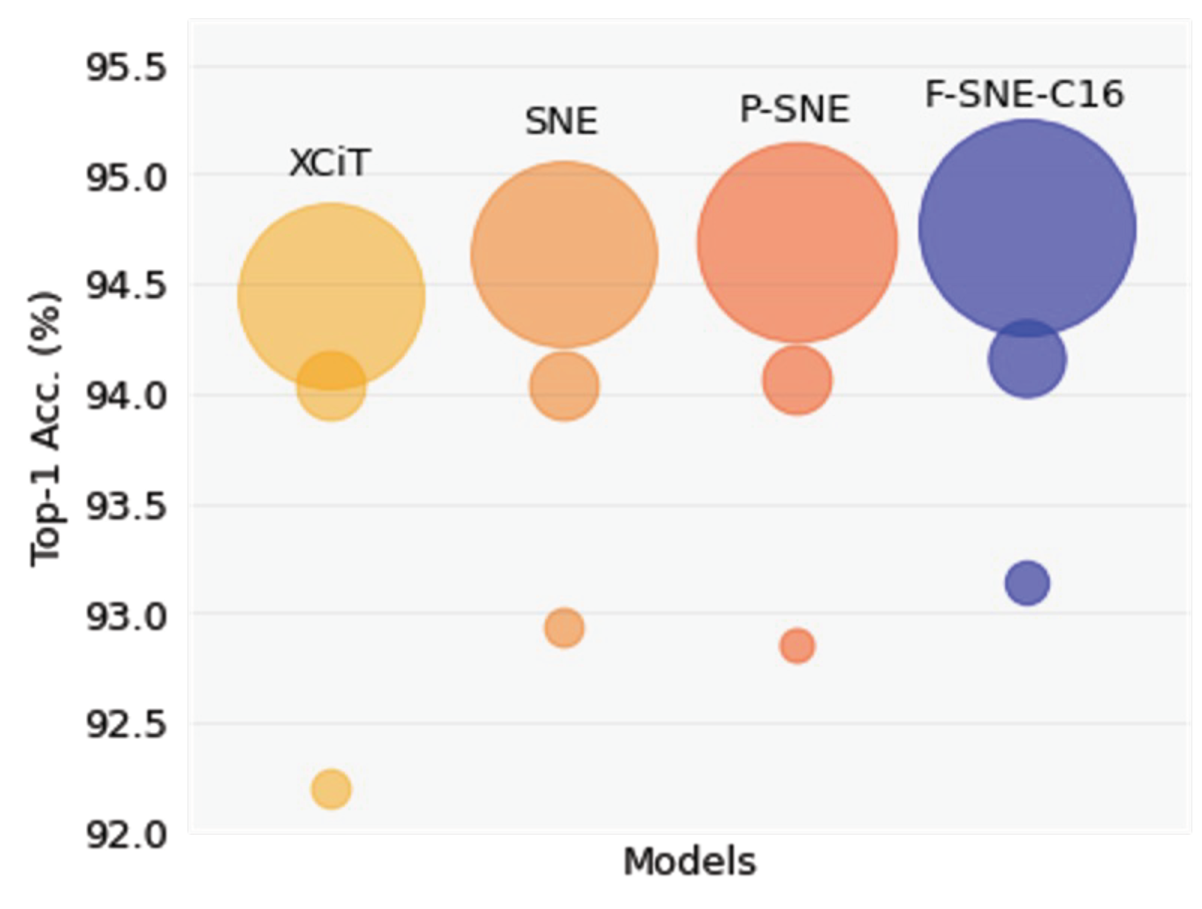
6.1. Which Structure Is the Best?

Among the three proposed structures, the F-SNE structure achieved the highest accuracies, especially in transfer learning tasks. As displayed in Figure 2, each structure of F-SNE coherently surpassed other structures with the corresponding computational cost. The F-SNE structure required a small increase in FLOPs to achieve this improvement but had fewer parameters compared to the XCiT, SNE, and P-SNE structures. According to these results, we can interpret that shared properties of the F-SNE structure have more generalized features within similar expressivity, and this results in the model’s ability to be easily adapted to downstream tasks. In addition, we observed that this improvement occurred obviously in smaller structures with limited generalization capacity.

6.2. Sharing or Unsharing Codes in F-SNE

Thanks to the code, the input token can be identified in the F-SNE structure for separately extracting Q, K, and V. In the F-SNE structure, codes $C_q$, $C_k$, and $C_v$ are shared among all embedding modules in the transformer model. This sharing can slightly reduce the total number of parameters. In addition, as presented in

Table 8. The cases of code sharing and unsharing were compared using the ImageNet-1k dataset. The numbers in brackets denote the number of total parameters for each model.

Model	Top-1 (%)
F-SNE-C8-S (Sharing)	70.82 (2.9 M)
F-SNE-C8-S (W/o Sharing)	70.28 (3.05 M)

, the generalization performance can be improved. Without sharing, the codes could have distinct values across the embedding modules, which could hinder finding the optimal code vectors for Q, K, and V. From this perspective, sharing could be a method for finding the optimal solution.

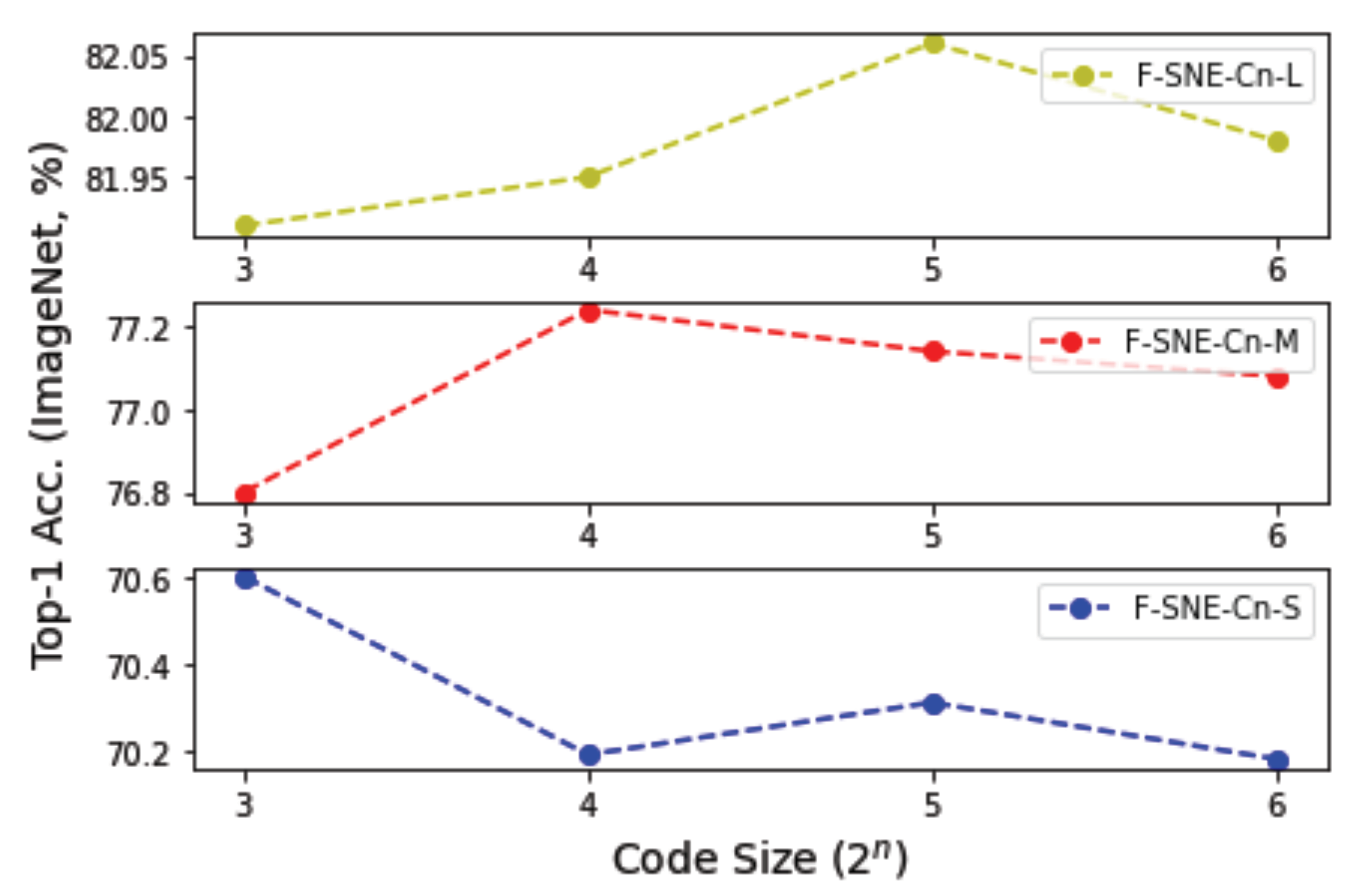
6.3. Code Size

Selecting an appropriate code size is critical for using the code $C_q$, $C_k$, and $C_v$ in the F-SNE structures. Therefore, we conducted experiments on different code sizes from 8 to 64 to determine an appropriate code size that can provide superior performance. As displayed in Figure 3, a code size of 8 achieved the best accuracy among S models, and a code size of 16 achieved the best accuracy among the M models. A code size of 32 achieved the best accuracy among L models. The M models have an embedding dimension of approximately 1.5 times, and the L models have three times the embedding dimension of the S models, as presented in Table 1. The results can be interpreted to mean that a larger code size is required when the embedding dimension of the model increases.

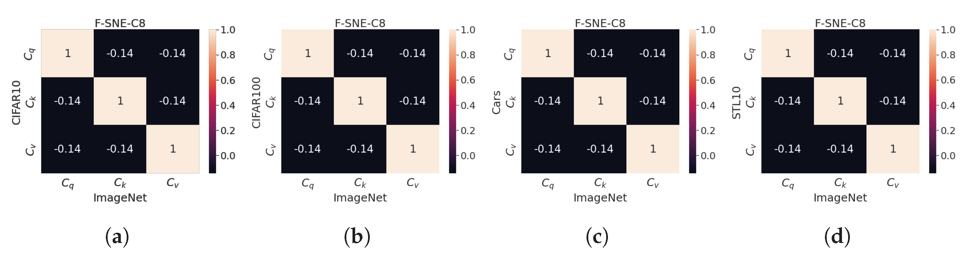
6.4. $C_Q,C_K$, and $C_V$ in Different Tasks

The optimal code values were initially found on the ImageNet-1k dataset, and subsequently, the computed code values were used as the initial codes for the downstream tasks. Even if the pre-trained codes were used, the code values might vary according to the tasks because the codes were updated using a back-propagation process using the downstream task dataset.

Figure 4 details the correlation values of codes extracted from each downstream task. Notably, the correlation matrices are similar even if the task is changed. The diagonal elements provide some information on the similarity between the same codes, and non-diagonal elements depict the similarity between different codes. Non-diagonal elements are close to zero, and each code of $C_q$, $C_k$, and $C_v$ tends to exhibit orthogonality. These results can be interpreted to indicate that $C_q$, $C_k$, and $C_v$ learn their inherent feature to be used as Q, K, and V, regardless of the task; furthermore, the values of the $l2$-norm for each dataset can be obtained, as presented in

Table 9. $l2$-norms of $C_q$, $C_k$, and $C_v$ are extracted from F-SNE-C8-S model according to the trained dataset. The codes exhibit similar $l2$-norm values regardless of the dataset.

Dataset	$||{\mathit{C}}_{\mathit{q}}||$	$||{\mathit{C}}_{\mathit{k}}||$	$||{\mathit{C}}_{\mathit{v}}||$
ImageNet	8.86	8.13	8.53
CIFAR-10	9.05	8.34	8.74
CIFAR-100	9.06	8.35	8.77
Cars	8.84	8.13	8.53
STL-10	8.86	8.14	8.56

. The codes of ImageNet-1k, Stanford Cars, and STL-10 exhibit similar $l2$-norm values, but CIFAR-10 and 100 exhibit distinct $l2$-norm values.

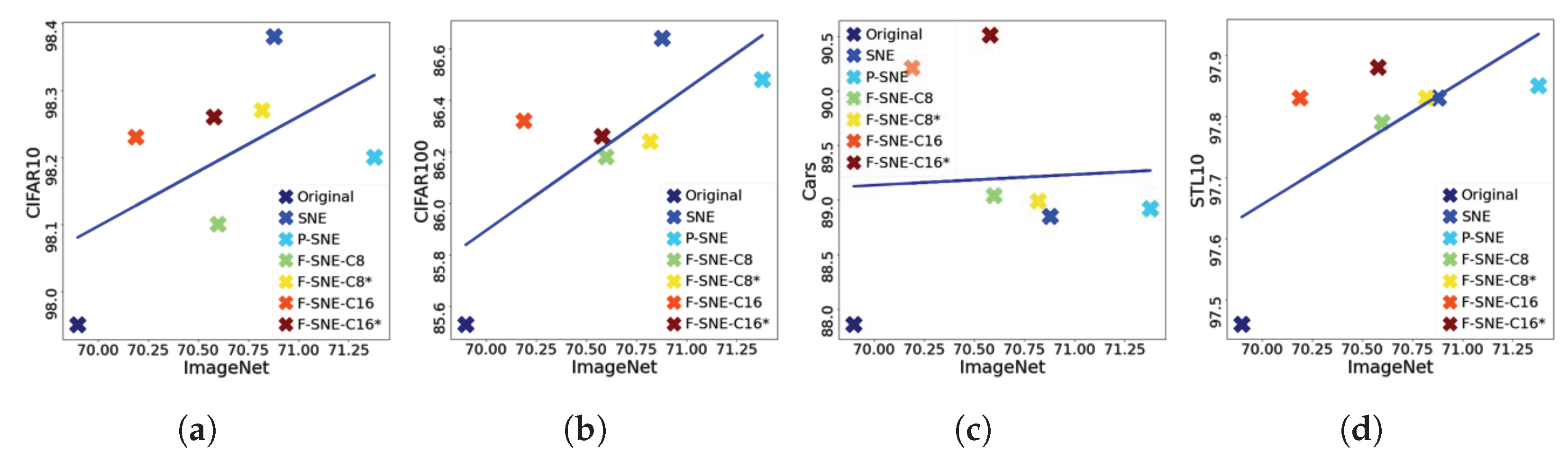
6.5. Do Better Imagenet Models Transfer Better?

Generally, better ImageNet models transfer better [45]. An experiment was conducted to verify whether this fact can be applied to our cases. As displayed in Figure 5, a correlation could be observed between performances on ImageNet and on downstream tasks. The correlation tendency is reflected by the domain difference between the upstream and downstream tasks. Thus, the tasks of the CIFAR-10, CIFAR-100, and STL-10 datasets are similar to the task of ImageNet. Therefore, these tasks exhibit high correlations between two tasks. However, correlations are difficult to observe in the Stanford Cars dataset.

7. Limitations

This study has several limitations that need to be addressed in future research. (1) While the proposed methods demonstrated significant performance improvements for tiny models, their impact on large models was relatively weak. Further research is required to improve their performances on larger models. (2) The evaluation was limited to classification, transfer learning, and out-of-distribution detection tasks. Future work should demonstrate the performances on other tasks, such as object detection and segmentation. (3) This study focused on supervised learning, but the potential benefits of the proposed methods in the context of self-supervised learning should be investigated. (4) Due to computational resource constraints, the experiments were conducted using ImageNet-1k or smaller datasets. Further evaluation on large-scale datasets is encouraged. (5) This study was unable to clearly interpret the precise function of the shared code. Additional analysis is needed to obtain a deeper understanding of the mechanisms of the proposed methods.

8. Conclusions

We proposed Q, K, and V vector embedding structures for XCiT. In the first embedding structure, two non-linear layers were used to embed the input token into separate non-linear spaces of Q, K, and V. In the second structure, a single layer was shared between the two layers. The results of the experiment revealed that sharing a single layer could improve generalization performance on ImageNet-1k. The third structure shares two layers with the Q, K, and V codes. The codes are trained via a back-propagation algorithm to minimize the loss. The structure can be used for improving the classification rates in several downstream tasks, such as CIFAR-100 and STL-10. Furthermore, the third structure could considerably improve OOD detection performance. Finally, we could improve the XCiT model under the fixed token dimensions using the proposed structures.

For future research, extensive experiments on a variety of vision tasks should be conducted to evaluate the effectiveness of the proposed structures. Moreover, a deeper analysis of the shared code is needed to elucidate its exact role and potential for improvement on larger models and datasets. By addressing these aspects, the proposed structures can be improved in the field of computer vision.

References

- Vaswani, A.; Shazeer, N.; Parmar, N.; Uszkoreit, J.; Jones, L.; Gomez, A.N.; Kaiser, Ł.; Polosukhin, I. Attention is all you need. In Proceedings of the Advances in Neural Information Processing Systems, Long Beach, CA, USA, 4–9 December 2017; pp. 5998–6008. [Google Scholar]
- Devlin, J.; Chang, M.W.; Lee, K.; Toutanova, K. BERT: Pre-training of Deep Bidirectional Transformers for Language Understanding. In Proceedings of the 2019 Conference of the North American Chapter of the Association for Computational Linguistics: Human Language Technologies, Volume 1 (Long and Short Papers); Association for Computational Linguistics: Cedarville, OH, USA, 2018; pp. 4171–4186. [Google Scholar]
- Radford, A.; Narasimhan, K.; Salimans, T.; Sutskever, I. Improving Language Understanding by Generative Pre-Training. 2018. Available online: https://www.cs.ubc.ca/~amuham01/LING530/papers/radford2018improving.pdf (accessed on 13 October 2021).
- Radford, A.; Wu, J.; Child, R.; Luan, D.; Amodei, D.; Sutskever, I. Language models are unsupervised multitask learners. OpenAI Blog 2019, 1, 9. [Google Scholar]
- Brown, T.B.; Mann, B.; Ryder, N.; Subbiah, M.; Kaplan, J.; Dhariwal, P.; Neelakantan, A.; Shyam, P.; Sastry, G.; Askell, A.; et al. Language models are few-shot learners. arXiv 2020, arXiv:2005.14165. [Google Scholar]
- Dosovitskiy, A.; Beyer, L.; Kolesnikov, A.; Weissenborn, D.; Zhai, X.; Unterthiner, T.; Dehghani, M.; Minderer, M.; Heigold, G.; Gelly, S.; et al. An image is worth 16x16 words: Transformers for image recognition at scale. arXiv 2020, arXiv:2010.11929. [Google Scholar]
- Carion, N.; Massa, F.; Synnaeve, G.; Usunier, N.; Kirillov, A.; Zagoruyko, S. End-to-End Object Detection with Transformers. In Proceedings of the Computer Vision—ECCV 2020, Glasgow, UK, 23–28 August 2020; Springer International Publishing: Cham, Switzerland, 2020; pp. 213–229. [Google Scholar]
- Touvron, H.; Cord, M.; Douze, M.; Massa, F.; Sablayrolles, A.; Jégou, H. Training Data-Efficient Image Transformers & Distillation Through Attention. arXiv 2020, arXiv:2012.12877. [Google Scholar]
- Ali, A.; Touvron, H.; Caron, M.; Bojanowski, P.; Douze, M.; Joulin, A.; Laptev, I.; Neverova, N.; Synnaeve, G.; Verbeek, J.; et al. XCiT: Cross-Covariance Image Transformers. In Proceedings of the Advances in Neural Information Processing Systems, Online, 6–14 December 2021; Ranzato, M., Beygelzimer, A., Dauphin, Y., Liang, P., Vaughan, J.W., Eds.; Curran Associates, Inc.: Red Hook, NY, USA, 2021; Volume 34, pp. 20014–20027. [Google Scholar]
- Wu, H.; Xiao, B.; Codella, N.; Liu, M.; Dai, X.; Yuan, L.; Zhang, L. Cvt: Introducing convolutions to vision transformers. arXiv 2021, arXiv:2103.15808. [Google Scholar]
- Yuan, L.; Chen, Y.; Wang, T.; Yu, W.; Shi, Y.; Jiang, Z.; Tay, F.E.; Feng, J.; Yan, S. Tokens-to-token vit: Training vision transformers from scratch on imagenet. arXiv 2021, arXiv:2101.11986. [Google Scholar]
- Yang, J.; Li, C.; Zhang, P.; Dai, X.; Xiao, B.; Yuan, L.; Gao, J. Focal self-attention for local-global interactions in vision transformers. arXiv 2021, arXiv:2107.00641. [Google Scholar]
- Yuan, L.; Hou, Q.; Jiang, Z.; Feng, J.; Yan, S. Volo: Vision outlooker for visual recognition. arXiv 2021, arXiv:2106.13112. [Google Scholar] [CrossRef] [PubMed]
- Deng, J.; Dong, W.; Socher, R.; Li, L.J.; Li, K.; Fei-Fei, L. ImageNet: A large-scale hierarchical image database. In Proceedings of the 2009 IEEE Conference on Computer Vision and Pattern Recognition, Miami, FL, USA, 20–25 June 2009; pp. 248–255. [Google Scholar]
- Krizhevsky, A.; Hinton, G. Learning Multiple Layers of Features from Tiny Images. 2009. Available online: http://www.cs.utoronto.ca/~kriz/learning-features-2009-TR.pdf (accessed on 22 March 2023).
- Krause, J.; Stark, M.; Deng, J.; Fei-Fei, L. 3d object representations for fine-grained categorization. In Proceedings of the IEEE International Conference on Computer Vision Workshops, Washington, DC, USA, 2–8 December 2013; pp. 554–561. [Google Scholar]
- Coates, A.; Ng, A.; Lee, H. An analysis of single-layer networks in unsupervised feature learning. In Proceedings of the Fourteenth International Conference on Artificial Intelligence and Statistics, Fort Lauderdale, FL, USA, 11–13 April 2011; pp. 215–223. [Google Scholar]
- Liu, Z.; Lin, Y.; Cao, Y.; Hu, H.; Wei, Y.; Zhang, Z.; Lin, S.; Guo, B. Swin transformer: Hierarchical vision transformer using shifted windows. arXiv 2021, arXiv:2103.14030. [Google Scholar]
- Yuan, K.; Guo, S.; Liu, Z.; Zhou, A.; Yu, F.; Wu, W. Incorporating convolution designs into visual transformers. arXiv 2021, arXiv:2103.11816. [Google Scholar]
- Xu, Y.; Zhang, Q.; Zhang, J.; Tao, D. ViTAE: Vision Transformer Advanced by Exploring Intrinsic Inductive Bias. arXiv 2021, arXiv:2106.03348. [Google Scholar]
- Steiner, A.; Kolesnikov, A.; Zhai, X.; Wightman, R.; Uszkoreit, J.; Beyer, L. How to train your ViT? Data, Augmentation, and Regularization in Vision Transformers. arXiv 2021, arXiv:2106.10270. [Google Scholar]
- d’Ascoli, S.; Touvron, H.; Leavitt, M.; Morcos, A.; Biroli, G.; Sagun, L. Convit: Improving vision transformers with soft convolutional inductive biases. arXiv 2021, arXiv:2103.10697. [Google Scholar] [CrossRef]
- Li, Y.; Zhang, K.; Cao, J.; Timofte, R.; Van Gool, L. Localvit: Bringing locality to vision transformers. arXiv 2021, arXiv:2104.05707. [Google Scholar]
- Sun, S.; Yue, X.; Bai, S.; Torr, P. Visual parser: Representing part-whole hierarchies with transformers. arXiv 2021, arXiv:2107.05790. [Google Scholar]
- Rao, Y.; Zhao, W.; Zhu, Z.; Lu, J.; Zhou, J. Global filter networks for image classification. Adv. Neural Inf. Process. Syst. 2021, 34, 980–993. [Google Scholar]
- Guibas, J.; Mardani, M.; Li, Z.; Tao, A.; Anandkumar, A.; Catanzaro, B. Efficient Token Mixing for Transformers via Adaptive Fourier Neural Operators. In Proceedings of the International Conference on Learning Representations, Virtual, 3–7 May 2021. [Google Scholar]
- Han, K.; Wang, Y.; Chen, H.; Chen, X.; Guo, J.; Liu, Z.; Tang, Y.; Xiao, A.; Xu, C.; Xu, Y.; et al. A survey on vision transformer. IEEE Trans. Pattern Anal. Mach. Intell. 2022, 45, 87–110. [Google Scholar] [CrossRef] [PubMed]
- Khan, S.; Naseer, M.; Hayat, M.; Zamir, S.W.; Khan, F.S.; Shah, M. Transformers in vision: A survey. ACM Comput. Surv. 2022, 54, 1–41. [Google Scholar] [CrossRef]
- Yu, F.; Seff, A.; Zhang, Y.; Song, S.; Funkhouser, T.; Xiao, J. Lsun: Construction of a large-scale image dataset using deep learning with humans in the loop. arXiv 2015, arXiv:1506.03365. [Google Scholar]
- Xu, P.; Ehinger, K.A.; Zhang, Y.; Finkelstein, A.; Kulkarni, S.R.; Xiao, J. Turkergaze: Crowdsourcing saliency with webcam based eye tracking. arXiv 2015, arXiv:1504.06755. [Google Scholar]
- Netzer, Y.; Wang, T.; Coates, A.; Bissacco, A.; Wu, B.; Ng, A.Y. Reading Digits in Natural Images with Unsupervised Feature Learning. 2011. Available online: http://ufldl.stanford.edu/housenumbers/nips2011_housenumbers.pdf (accessed on 22 March 2023).
- Cimpoi, M.; Maji, S.; Kokkinos, I.; Mohamed, S.; Vedaldi, A. Describing textures in the wild. In Proceedings of the IEEE Conference on Computer Vision and Pattern Recognition, Columbus, OH, USA, 23–28 June 2014; pp. 3606–3613. [Google Scholar]
- Chen, J.; Li, Y.; Wu, X.; Liang, Y.; Jha, S. Robust out-of-distribution detection for neural networks. arXiv 2020, arXiv:2003.09711. [Google Scholar]
- Chen, Y.; Dai, X.; Chen, D.; Liu, M.; Dong, X.; Yuan, L.; Liu, Z. Mobile-Former: Bridging MobileNet and Transformer. arXiv 2021, arXiv:2108.05895. [Google Scholar]
- Wang, W.; Xie, E.; Li, X.; Fan, D.P.; Song, K.; Liang, D.; Lu, T.; Luo, P.; Shao, L. Pvt v2: Improved baselines with pyramid vision transformer. Comput. Vis. Media 2022, 8, 415–424. [Google Scholar] [CrossRef]
- Xu, W.; Xu, Y.; Chang, T.; Tu, Z. Co-Scale Conv-Attentional Image Transformers. In Proceedings of the IEEE/CVF International Conference on Computer Vision (ICCV), Montreal, QC, Canada, 10–17 October 2021; pp. 9981–9990. [Google Scholar]
- Heo, B.; Yun, S.; Han, D.; Chun, S.; Choe, J.; Oh, S.J. Rethinking spatial dimensions of vision transformers. arXiv 2021, arXiv:2103.16302. [Google Scholar]
- Yan, H.; Li, Z.; Li, W.; Wang, C.; Wu, M.; Zhang, C. ConTNet: Why not use convolution and transformer at the same time? arXiv 2021, arXiv:2104.13497. [Google Scholar]
- Zhang, Q.; Yang, Y.B. ResT: An efficient transformer for visual recognition. Adv. Neural Inf. Process. Syst. 2021, 34, 15475–15485. [Google Scholar]
- Touvron, H.; Cord, M.; Sablayrolles, A.; Synnaeve, G.; Jégou, H. Going Deeper With Image Transformers. In Proceedings of the IEEE/CVF International Conference on Computer Vision (ICCV), Montreal, QC, Canada, 10–17 October 2021; pp. 32–42. [Google Scholar]
- Radosavovic, I.; Kosaraju, R.P.; Girshick, R.; He, K.; Dollár, P. Designing network design spaces. In Proceedings of the IEEE/CVF Conference on Computer Vision and Pattern Recognition, Seattle, WA, USA, 14–18 June 2020; pp. 10428–10436. [Google Scholar]
- Hoffer, E.; Ben-Nun, T.; Hubara, I.; Giladi, N.; Hoefler, T.; Soudry, D. Augment your batch: Improving generalization through instance repetition. In Proceedings of the IEEE/CVF Conference on Computer Vision and Pattern Recognition, Seattle, WA, USA, 13–19 June 2020; pp. 8129–8138. [Google Scholar]
- Hendrycks, D.; Gimpel, K. A baseline for detecting misclassified and out-of-distribution examples in neural networks. arXiv 2016, arXiv:1610.02136. [Google Scholar]
- Lee, K.; Lee, H.; Lee, K.; Shin, J. Training confidence-calibrated classifiers for detecting out-of-distribution samples. arXiv 2017, arXiv:1711.09325. [Google Scholar]
- Kornblith, S.; Shlens, J.; Le, Q.V. Do better imagenet models transfer better? In Proceedings of the IEEE/CVF Conference on Computer Vision and Pattern Recognition, Long Beach, CA, USA, 15–20 June 2019; pp. 2661–2671. [Google Scholar]
Figure 1.
Four types of Q, K, and V embedding methods are shown. (a) The figure depicts conventional embedding used in the standard transformer encoder. (b) Separate non-linear embedding utilizes a two-layer embedding, including non-linearity functions (e.g., ReLU). (c) Partially shared non-linear embedding includes a weight-sharing linear layer. The weight-sharing layer is depicted as the gray dotted line block, and it follows after the separated linear layer and ReLU. (d) Fully shared non-linear embedding includes two weight-sharing linear layers, also depicted as a gray dotted line, with ReLU. In this case, trainable codes of Q, K, V (, , and ) are concatenated to the input tokens.
Figure 2.
Performances were compared among proposed structures. Averaged top-1 accuracies of transfer learning were used. Circle size corresponds to FLOPs of each structure.
Figure 3.
Top-1 accuracies on ImageNet-1k of F-SNE-Cn-S, F-SNE-Cn-M, and F-SNE-Cn-L structures were compared with respect to code sizes from 8 to 64. Results of F-SNE-Cn-S, F-SNE-Cn-M, and F-SNE-Cn-L structures are organized from bottom to top.
Figure 4.
-normalized , , and are dot-producted according to the trained datasets. “IMNet”, “C10”, “C100”, and “S10” denote ImageNet, CIFAR-10, CIFAR-100, and STL-10, respectively. , , and are extracted from the F-SNE-C8-S model. (a) IMNet-C10. (b) IMNet-C100. (c) IMNet-Cars. (d) IMNet-S10.
Figure 5.
Correlation between pre-training and transfer learning performances is plotted. S models are used. ‘X’ markers denote the accuracies of each model, and the blue line denotes the regression slope of the results. In contrast to other correlated plots, the results on the Stanford Cars dataset are not correlated with the results on the ImageNet dataset. Best viewed in color. (a) IMNet-C10. (b) IMNet-C100. (c) IMNet-Cars. (d) IMNet-S10.