Abstract
This paper studies the problem of the event-triggered control of nonaffine stochastic nonlinear systems with actuator hysteresis. The echo state network (ESN) is introduced to approximate an unknown nonlinear function. The command filtering technology is used to avoid the derivation of the virtual controller in the controller design process and tries to solve the problem of complexity explosion in the traditional method. Based on Lyapunov’s finite-time stability theory, the proposed method verifies the stability of non-affine stochastic nonlinear systems. It is proved that the proposed controller method can guarantee that all of the signals in the closed-loop system are bounded, and the tracking error can converge to a minimal neighborhood of zero even if there exists an actuator hysteresis. The effectiveness of the proposed method is demonstrated by the simulation example. The simulation results show that the proposed method is effective.
Keywords:
stochastic nonaffine systems; adaptive control; echo state network (ESN); event-triggered; hysteresis MSC:
93E15
1. Introduction
With the development of society, system control plays a vital role in many fields such as the military, as well as industrial production. Linear systems are not only theoretically studied but also widely applied [1]. However, in real life the system can be easily affected by uncertain factors. As a result, the system will be nonlinear [2]. With the passage of time, the traditional nonlinear system cannot meet the needs of social development. The research of complex systems has increasingly attracted scholars’ attention. Due to the influence of stochastic disturbances, the actual systems are embodied with randomness. Therefore, the study of stochastic nonlinear systems is of great significance and practical value. Regarding stochastic nonlinear systems, there are also many systems whose state variables or actual controls are not clearly represented. Therefore, the system often has a non-affine appearance.
Stochastic nonaffine nonlinear systems can be applied to many fields, including aerospace systems and robot operations. In [3,4], the unknown nonaffine input is transformed into a partially affine form using the mean value theorem, and all signals in a closed loop system are bounded. Therefore, the same method is used in this paper to deal with the nonaffine problem of control variables by using the mean value theorem and transform the nonaffine system into a simple standard stochastic nonlinear system.
For some nonlinear systems, backstepping control is a powerful and typical control method for parametric uncertainty [5,6]. The backstepping method was proposed in [7]. A controller was established by constructing the quadratic Lyapunov function. So far, many new algorithms have been created to solve the nonlinear system problems. The backstepping control strategy is an effective method for solving uncertain systems, and it has been widely used. However, the traditional backstepping design method also has disadvantages. The complexity of the control design and stability increase exponentially with the increase in the system order, that is, each calculation step of the virtual controller may lead to the “explosion of complexity”. In order to solve this problem, ref. [8] developed a dynamic surface control (DSC) technique that introduced a low-pass filter in each control input for the first time. The above DSC technique does not take the error of the first-order filter into consideration, which may affect the precision and accuracy of the system. The command filter control (CFC) adopted in this paper utilizes an error compensation mechanism at each step of the command filter to reduce the influence of filter errors.
The control of nonlinear systems with unknown hysteretic nonlinearity has always been a popular topic. Hysteretic nonlinearity is very common in the actuation of smart materials, such as piezoelectric materials and shape memory alloys. Nonlinearity and hysteresis have a remarkable influence on the system, causing it to become unstable [9]. Robust adaptive control and adaptive inversion control for a class of nonlinear systems with unknown hysteresis are studied in [10,11]. The approach presented in [12,13,14] cannot solve the control problem of nonlinear systems with a post-performance period. Therefore, it is a great challenge to solve the problem of stochastic nonaffine systems with actuator hysteresis.
In addition, with the development of the network, event-triggered control has become popular as it can effectively reduce the waste of communication and resources. The article [15] considers the problem of adaptive fuzzy switching event-triggered control for a class of nonaffine stochastic systems with periodic actuator faults. The paper [16] considers the event-triggered adaptive tracking control for RDE systems with coexisting parametric uncertainties and severe nonlinearities. In traditional control design, the output of the controller is transmitted to the actuators, which may generate redundant update signals and then cause waste of the communication network [17]. Thus, these issues motivate the development of event-triggered strategies. In [18], an event-triggered strategy is developed for nonlinear uncertain systems, in which the uncertain part is represented by the product of known functions and unknown parameters. In [19], for nonlinear uncertain systems, an event-triggered strategy using neural networks to approximate the uncertain part is proposed. The fixed threshold strategy and the relative threshold strategy are discussed in [20,21] since the threshold of the fixed threshold strategy is a constant but the control signal of the actual system is not static. If the amplitude of the control signal is too large, it will lead to system instability. A neural adaptive event-triggered strategy that greatly saves communication resources while ensuring system performance is proposed [22]. Therefore, this paper employs the relative threshold strategy. However, to the best of our knowledge, there are currently few methods to solve the event-triggered problem of stochastic nonaffine systems with actuator hysteresis, thus motivating our current work.
Based on the above discussion, a neural network control design for stochastic non-affine nonlinear systems with event triggering and actuator hysteresis is constructed, and the echo state network (ESN) is introduced to approximate the unknown nonlinear functions. In other papers, such as [23,24], the radial basis function neural network (RBFNN) structure is used to approximate the unknown functions. In [25], a recurrent neural network (RNN) is proposed to approximate the unknown function. However, the former can only rely on the current input, while the latter requires higher computational costs. This paper proposes a simple method to approximate the unknown functions by using the echo state network, which is better than other methods and can be trained easily.
(1) The ESN network is used to approximate the unknown function generated during the design process. Compared with RBFNN in [24], ESN has better stability than the RBFNN network without a complex training process. Compared with RNNS in [25], weight updating does not require a particularly high computational cost, and the training speed is faster than that of RNNS. Therefore, this paper uses the echo state network as a new approach to approximate the unknown function more simply and accurately in the controller design, which greatly reduces the calculation cost.
(2) This paper introduces the actuator hysteresis into the nonaffine system and uses the mean value theorem to transform the nonaffine stochastic nonlinear system into a stochastic nonlinear system. Compared with the nonlinear control problem of [12,13,14], actuator hysteresis has not been fully considered. This paper greatly reduces the complexity of the system and solves the problem of actuator hysteresis in nonlinear systems.
(3) Compared with [17] and [18], the problem of resource waste in the communication process is solved by designing an event-triggered controller, and the relative threshold is used to ensure the stability of the system in the design process.
The rest of the paper is as follows. In Section 2, more information of stochastic nonaffine systems and ESN will be further illustrated. Section 3 introduces the design method of the event trigger controller and provides the stability analysis of the system. Section 4 describes the simulation process to verify the effectiveness of the proposed method. In the end, the conclusions are given in Section 5.
2. Preliminaries
2.1. Problem Formulation
For the following stochastic nonlinear system
where is the system state, and indicate the locally Lipschitz functions with . represents an r-dimensional standard Wiener process.
Definition 1 ([26]).
For any given function in , define the differential operator as
with Tr as the matrix trace.
Lemma 1 ([27]).
For the stochastic nonlinear system (1), there is a Lyapunov function , and . When , function meets the following requirements:
when , two normal numbers, α and Γ, exist. System (1) has a unique strong solution, all of the signals in the closed-loop system are bounded in probability, and the system satisfies
For the following class of stochastic nonaffine systems with actuator hysteresis:
where , is the system input, and is the system output. denotes the hysteresis nonlinearities. is a r-dimensional standard Brownian motion defined in the complete probability space . denotes the sample space. F denotes the -field. P denotes the probability measure. and represent the unknown smooth functions.
The control signal v and the hysteresis type of nonlinearity in the Formula (5) are defined as
where , , and are designed parameters; is the slope of lines; and guarantee .
Dynamics is used to simulate the backlash-like hysteresis, and additional parameters are put up as , , and , and the initial conditions as , .
Moreover, Equation (6) can be properly handled as follows:
where and . are bounded and satisfy , and is the unknown constant.
For the sake of simplicity, the time variable t will be omitted below. Based on mean value theorem, the smooth nonlinear function can be changed into the form as
where , , , , . With , the original system (5) can be described as follows:
Assumption A1.
The sign of in is known for . Without a loss of generality, and for the convenience of analysis and design, assume that
Assumption A2.
The reference signal and its time derivatives up to the n th order are continuous and bounded.
2.2. Echo State Network
The following form of ESN continuous-time dynamics is given [28]
where the activation function of the dynamic reservoirs . is a positive number representing the stored neuron’s leakage rate; denotes a hyperbolic tangent function. and represent the input and internal connection weight matrices, respectively. represents feedback connection weight matrices; u means the external input with K-dimensional. The output signal’s equation is defined as follows:
with being the weight matrix of output.
It can be seen in [29] that the output of RNNs can be used to approximate any continuous function, which indicates that there is an ESN system, as shown in Equation (11) above. Therefore, as for any given continuous smooth function , the below inequality is true
In addition, the function can be approached by
where is the ideal weight matrix satisfying , and is bounded to satisfy . stands for the activation function where is chosen as
where , , , and are the constant parameters, and is bounded by and .
On account of the fact the weight W is generally uncharted in reality, to guarantee the asymptotic tracking performance, the estimated value of W, (expressed as ), is employed and updated by designing adaptive laws online.
Remark 1.
From the above discussions, it can be deduced that ESN is an optional tool for function approximation and can be replaced with any other approximation techniques, for instance, RBFNNs, FLSs, and others [30,31]. Compared to RBFNNs, ESN does not need to adjust the weights between the input layer and the hidden layer, and the training is simple and accurate.
Lemma 2.
The hyperbolic function holds the following property [32]:
where , , and .
Lemma 3.
The Young’s inequality is described as [33]:
where , , , and .
3. Event-Triggered Adaptive Controller Design
In the backstepping design process, the following tracking errors are defined as
where , represents the reference signals, virtual controllers are the input signals of the command filters, and the outputs signal of the filters are . The command filters are defined as follows:
If the input signal satisfies and for all , where , , and , for any , the filter design parameters exist, and the following inequality holds: .
In order to reduce the influence of command filtering on error, the following new tracking error signals are defined by using the error compensation mechanism:
where , the compensating signals are designed as
where are design constants and .
Step 1: The following can be obtained from (17)
Choose the Lyapunov candidate function as follows:
where is a design constant, and , denotes the estimation of .
According to (3) and Definition 1, we have
By using Young’s inequality, the following inequality holds:
where is a designed constant. Substituting (26) into (25), we have
where and . By the ESN (13), the uncharted nonlinear function can be approximated to , is the approximation error satisfying , and .
By using Lemma 3, the following inequality holds:
where , is a designed parameter.
The compensating signal can be designed as follows:
with .
By using Young’s inequality and Assumption 1, the inequality is as follows:
The virtual control signal is devised as follows:
The designed adaptive law is as follows:
Step i Based on (17), the following formula comes into existence:
Select the following candidate Lyapunov function:
where are designed constants, , , are expressed as an estimate of , and . According to Definition 1 and (38), the conclusions can be drawn as follows:
According to Lemma 3, the following equation is true
and are the designed normal numbers. By using (41), (40) can be rewritten as follows:
where and . For any given , exists, such that , , where denotes the approximation error.
By using Young’s inequality, it follows that
where and is a positive constant.
By substituting (43) into (42) yields, we obtain that
The compensation signal is designed as
with , substituting (45) into (44), the following can be obtained:
Based on Young’s inequality, we have
Design the virtual control signals as follows:
Design the adaptive laws as follows:
Design of Event-Triggered Controller
The event-triggered strategy is described as follows:
where , and is the designed parameter.
Remark 2.
Whensoever the event-triggered mechanism is triggered, the time is marked as and the control value is applied to the system. During the time , the control signal holds as a constant.
From (52), we can draw a conclusion , , and is the time-varying parameter. As a result, the equation is obtained as follows:
Step n: From (17), we can obtain
Choose a Lyapunov function as
where is a designed constant, and , is the estimation of , and .
According to Definition 1 and (54), it can be deduced that
Design the compensating signal as follows:
By Assumption 1, and , the inequalities can be held as
Based on Lemma 3, we can obtain
Based on Young’s inequality, one has
During the process of designing virtual controllers, the unknown nonlinear function is approximated by ESNs, where . By using the universal approximation capability of ESN (13), for any given , an ESN always exist, such that , where and is the approxomation error satisfying .
Baesd on Lemma 3, the inequality holds that
where , is a given positive constant.
It can be known from Young’s inequality that the inequality holds
Design the virtual control signal as follows:
We design the adaptive law as follows:
By using Young’s inequality,
Theorem 1.
Consider a class of stochastic nonaffine nonlinear system (5) under Assumptions 1 and 2. The packaged unknown can be approximated by the ESN networks by which the approximating error is bounded. Event-triggered strategy (52); adaptive controllers (33), (48), (62), and (73); and adaptive laws (36), (50), and (73) in the closed-loop system are bounded in probability. Specifically, the tracking error will be converged as
with , and .
Proof.
Define , it could be obtained from (76) that
Remark 3.
An adaptive neural finite-time-event-triggered consensus tracking problem is studied for nonlinear multi-agent systems (MASs) under directed graphs [34]. In stochastic systems such as [35,36], there is no error graph, but the tracking graph cannot completely overlap. On the one hand, the tracking error cannot completely converge to zero because of different systems. On the other hand, the tracking error cannot completely converge to zero in finite time. Inspired by [34], the following research will help the stochastic system tracking error converge to zero.
4. Simulation Results
To illustrate the effectiveness of the proposed control method, we choose the following stochastic nonaffine nonlinear systems:
where , are the system states.
The command filter is devised as
We design the compensating signals as
The virtual controllers , , and updating laws , are designed as
The event-triggered controller and actual controller u are designed as
and the event-triggered mechanism is as follows: .
We choose the initial condition and main parameters as follows: , , , , , , , . The reference , , , , , , , , , , , , , , , , , , .
The final simulation results are represented in Figure 1, Figure 2, Figure 3, Figure 4 and Figure 5. The output of system can keep up with the desired trajectory within a very small error range, where T = 20 s; Figure 1 expresses the tracking diagram for reference and output y, and the error trajectory is shown in Figure 2. It can be clearly indicated that the tracking error is in a minimal neighborhood of zero. Figure 3 shows the triggered events. Figure 4 shows that the adaptive parameters and , and the control signal is shown in Figure 5.
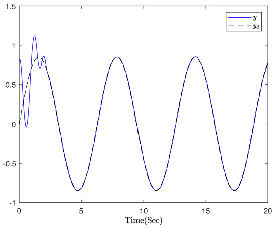
Figure 1.
System output and reference signal .
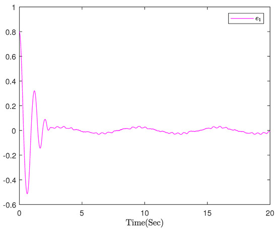
Figure 2.
The trajectory of error .
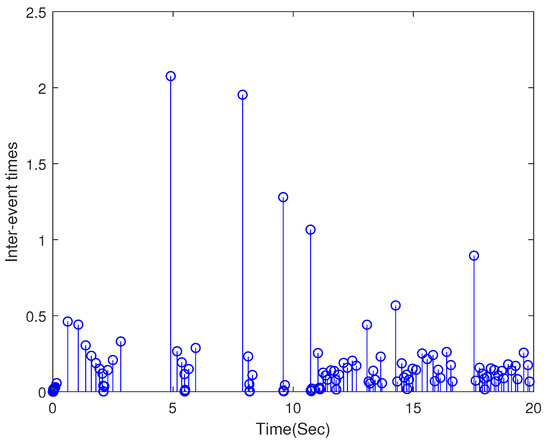
Figure 3.
The trigger time interval.
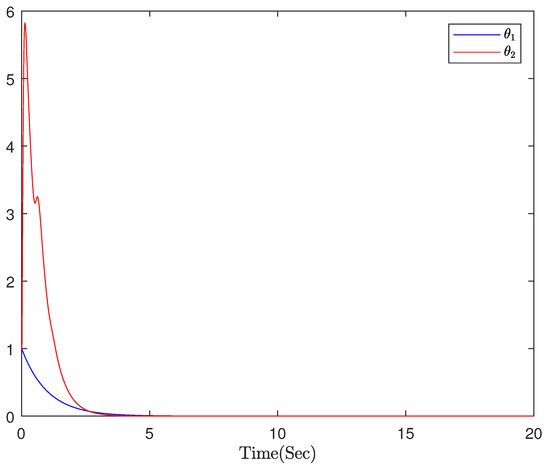
Figure 4.
Adaptive parameters and .
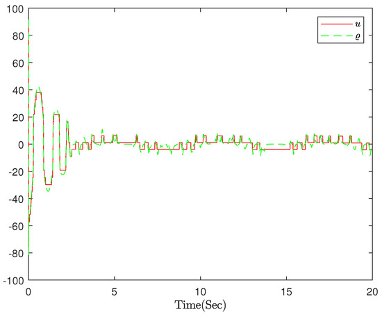
Figure 5.
Comparison between event-triggered control signal u and intermediate control signal .
5. Conclusions
In this paper, a control scheme based on error compensation for command filtering is proposed to solve the tracking control problem of stochastic nonaffine nonlinear systems with event triggering and actuator hysteresis. Using ESN to approximate unknown functions is simpler than using RBF neural networks or other methods. The “explosion of complexity” is solved by command-filtering technology, and the error caused by command filtering is solved by the compensation signal. By utilizing the event-triggered control, the waste of communication resources is reduced. Considering the existence of hysteretic nonlinearity, the proposed control scheme can ensure that the signals in the closed loop are all bounded. Finally, the effectiveness of the method is proved by the simulation results.
Author Contributions
Conceptualization, X.L.; software, M.L.; resources, T.T.; writing—original draft, Z.Q.; and writing—review & editing, S.L. All authors have read and agreed to the published version of the manuscript.
Funding
Work supported by the National Natural Science Foundation of China (61773074) and Key project of Education Department of Liaoning Province (LJKZZ20220118).
Conflicts of Interest
The authors declare no conflict of interest.
References
- Hespanha, J.P. Linear Systems Theory; Princeton University Press: Princeton, NJ, USA, 2018. [Google Scholar]
- Vander, V.; Wallace, E.T. Multiple-Input Describing Functions and Nonlinear System Design; McGraw Hill: New York, NY, USA, 1968. [Google Scholar]
- Chen, M.; Wang, H.; Liu, X.; Hayat, T.; Alsaadi, F.E. Adaptive finite-time dynamic surface tracking control of nonaffine nonlinear systems with dead zone. Neurocomputing 2019, 366, 66–73. [Google Scholar] [CrossRef]
- Ge, S.S.; Zhang, J. Neural-network control of nonaffine nonlinear system with zero dynamics by state and output feedback. IEEE Trans. Neural Netw. 2003, 10, 900–918. [Google Scholar]
- Kanellakopoulos, I.; Kokotovic, P.V.; Morse, A.S. Systematic design of adaptive controllers for feedback linearizable systems. In Proceedings of the 1991 American Control Conference, Boston, MA, USA, 26–28 June 1991; pp. 649–654. [Google Scholar]
- Mokhtari, M.; Chara, K.; Golea, N. Adaptive Neural Network Control for a Simple Pendulum Using Backstepping with Uncertainties. Int. J. Adv. Sci. Technol. (IJAST) 2014, 10, 81–94. [Google Scholar] [CrossRef]
- Pan, Z.; Basar, T. Adaptive controller design for tracking and disturbance attenuation in parametric strict-feedback nonlinear systems. IEEE Trans. Autom. Control. 1998, 43, 1066–1083. [Google Scholar] [CrossRef]
- Swaroop, D.; Hedrick, J.K.; Yip, P.P.; Gerdes, J.C. Dynamic surface control for a class of nonlinear systems. IEEE Trans. Autom. Control. 2000, 45, 1893–1899. [Google Scholar] [CrossRef]
- Tao, G.; Kokotovic, P.V. Adaptive control of plants with unknown hystereses. IEEE Trans. Autom. Control. 1995, 40, 200–212. [Google Scholar] [CrossRef]
- Su, C.Y.; Stepanenko, Y.; Svoboda, J.; Leung, T.P. Robust adaptive control of a class of nonlinear systems with unknown backlash-like hysteresis. IEEE Trans. Autom. Control. 2000, 45, 2427–2432. [Google Scholar] [CrossRef]
- Zhou, J.; Wen, C.; Zhang, Y. Adaptive backstepping control of a class of uncertain nonlinear systems with unknown backlash-like hysteresis. IEEE Trans. Autom. Control. 2004, 49, 1751–1759. [Google Scholar] [CrossRef]
- Zhang, T.; Xia, M.; Yi, Y. Adaptive neural dynamic surface control of strict-feedback nonlinear systems with full state constraints and unmodeled dynamics. Automatica 2017, 81, 232–239. [Google Scholar] [CrossRef]
- Liu, Z.; Lai, G.; Zhang, Y.; Chen, C.L.P. Adaptive neural output feedback control of output-constrained nonlinear systems with unknown output nonlinearity. IEEE Trans. Neural Netw. Learn. Syst. 2015, 26, 1789–1802. [Google Scholar]
- Sun, K.; Mou, S.; Qiu, J.; Wang, T.; Gao, H. Adaptive fuzzy control for nontriangular structural stochastic switched nonlinear systems with full state constraints. IEEE Trans. Fuzzy Syst. 2018, 27, 1587–1601. [Google Scholar] [CrossRef]
- Wu, Y.; Zhang, G.; Wu, L.B. Finite-Time Adaptive Fuzzy Switching Event-Triggered Control for Nonaffine Stochastic Systems. IEEE Trans. Fuzzy Syst. 2022, 30, 5261–5275. [Google Scholar] [CrossRef]
- Zhang, H.; Xi, R.; Wang, Y.; Sun, S.; Sun, J. Event-triggered adaptive tracking control for random systems with coexisting parametric uncertainties and severe nonlinearities. IEEE Trans. Autom. Control. 2021, 67, 2011–2018. [Google Scholar] [CrossRef]
- Gupta, R.A.; Chow, M.Y. Overview of networked control systems. Netw. Control. Syst. 2008, 1–23. [Google Scholar]
- Caiazzo, B.; Lui, D.G.; Petrillo, A.; Santini, S. Distributed Robust Finite-Time PID Control for the Leader-Following Consensus of Uncertain Multi-Agent Systems with Communication Delay. In Proceedings of the 2021 29th Mediterranean Conference on Control and Automation (MED), PUGLIA, Italy, 15 July 2021; pp. 759–764. [Google Scholar]
- Wang, J.; Liu, Z.; Zhang, Y.; Chen, C.P.; Lai, G. Adaptive neural control of a class of stochastic nonlinear uncertain systems with guaranteed transient performance. IEEE Trans. Cybern. 2019, 50, 2971–2981. [Google Scholar] [CrossRef] [PubMed]
- Garcia, E.; Antsaklis, P.J. Model-Based Event-Triggered Control with Time-Varying Network Delays. In Proceedings of the 2011 50th IEEE Conference on Decision and Control and European Control Conference, Orlando, FL, USA, 12–15 December 2011; pp. 1650–1655. [Google Scholar]
- Tabuada, P. Event-triggered real-time scheduling of stabilizing control tasks. IEEE Trans. Autom. Control. 2007, 52, 1680–1685. [Google Scholar] [CrossRef]
- Li, Y.X.; Hu, X.Y.; Ahn, C.K.; Hou, Z.S.; Kang, H.H. Event-based adaptive neural asymptotic tracking control for networked nonlinear stochastic systems. IEEE Trans. Netw. Sci. Eng. 2022, 9, 2290–2300. [Google Scholar] [CrossRef]
- Wei, J.; Hu, Y.; Sun, M. Adaptive iterative learning control for a class of nonlinear time-varying systems with unknown delays and input dead-zone. IEEE/CAA J. Autom. Sin. 2014, 1, 302–314. [Google Scholar]
- Sun, M.; Wu, T.; Chen, L.; Zhang, G. Neural AILC for error tracking against arbitrary initial shifts. IEEE Trans. Neural Netw. Learn. Syst. 2017, 29, 2705–2716. [Google Scholar] [CrossRef]
- Ku, C.C.; Lee, K.Y. Diagonal recurrent neural networks for dynamic systems control. IEEE Trans. Neural Netw. 1995, 6, 144–156. [Google Scholar]
- Wang, H.; Liu, K.; Liu, X.; Chen, B.; Lin, C. Neural-based adaptive output-feedback control for a class of nonstrict-feedback stochastic nonlinear systems. IEEE Trans. Cybern. 2014, 45, 1977–1987. [Google Scholar] [CrossRef] [PubMed]
- Sui, S.; Chen, C.P.; Tong, S. Fuzzy adaptive finite-time control design for nontriangular stochastic nonlinear systems. IEEE Trans. Fuzzy Syst. 2018, 27, 172–184. [Google Scholar] [CrossRef]
- Jaeger, H.; Lukoševičius, M.; Popovici, D. Optimization and applications of echo state networks with leaky-integrator neurons. IEEE Trans. Neural Netw. 2007, 20, 335–352. [Google Scholar] [CrossRef]
- Funahashi, K.I.; Nakamura, Y. Approximation of dynamical systems by continuous time recurrent neural networks. Neural Netw. 1993, 6, 801–806. [Google Scholar] [CrossRef]
- Chen, Q.; Shi, H.; Sun, M. Echo state network-based backstepping adaptive iterative learning control for strict-feedback systems: An error-tracking approach. IEEE Trans. Cybern. 2019, 50, 3009–3022. [Google Scholar] [CrossRef]
- Luo, S.; Li, S.; Tajaddodianfar, F.; Hu, J. Anti-Oscillation and Chaos Control of the Fractional-Order Brushless DC Motor System via Adaptive Echo State Networks: An Error-Tracking Approach; Elsevier: Amsterdam, The Netherlands, 2018; pp. 6435–6453. [Google Scholar]
- Ren, B.; San, P.P.; Ge, S.S.; Lee, T.H. Adaptive dynamic surface control for a class of strict-feedback nonlinear systems with unknown backlash-like hysteresis. In Proceedings of the 2009 American Control Conference, St. Louis, MI, USA, 10–12 June 2009; pp. 4482–4487. [Google Scholar]
- Wu, L.B.; Park, J.H.; Zhao, N.N. Robust adaptive fault-tolerant tracking control for nonaffine stochastic nonlinear systems with full-state constraints. IEEE Trans. Cybern. 2019, 50, 3793–3805. [Google Scholar] [CrossRef]
- Li, Y.; Li, Y.X.; Tong, S. Event-based finite-time control for nonlinear multi-agent systems with asymptotic tracking. IEEE Trans. Autom. Control. 2022, 3793–3805. [Google Scholar] [CrossRef]
- Ouyang, X.Y.; Wu, L.B.; Zhao, N.N.; Gao, C. Event-triggered adaptive prescribed performance control for a class of pure-feedback stochastic nonlinear systems with input saturation constraints. Int. J. Syst. Sci. 2020, 51, 2238–2257. [Google Scholar] [CrossRef]
- Sun, Y.; Chen, B.; Lin, C.; Wang, H.; Zhou, S. Adaptive neural control for a class of stochastic nonlinear systems by backstepping approach. Inf. Sci. 2016, 369, 748–764. [Google Scholar] [CrossRef]
Disclaimer/Publisher’s Note: The statements, opinions and data contained in all publications are solely those of the individual author(s) and contributor(s) and not of MDPI and/or the editor(s). MDPI and/or the editor(s) disclaim responsibility for any injury to people or property resulting from any ideas, methods, instructions or products referred to in the content. |
© 2023 by the authors. Licensee MDPI, Basel, Switzerland. This article is an open access article distributed under the terms and conditions of the Creative Commons Attribution (CC BY) license (https://creativecommons.org/licenses/by/4.0/).