Abstract
The Basrah Refinery, Iraq, similarly to other refineries, is subject to several industrial constraints. Therefore, the main challenge is to optimize the parameters of the level controller of the process unit tanks. In this paper, a PI controller is designed for these important processes in the Basrah Refinery, which is a separator drum (D5204). Furthermore, the improvement of the PI controller is achieved under several constraints, such as the inlet liquid flow rate to tank (m2) and valve opening in yi%, by using two different techniques: the first one is conducted using a closed-Loop PID auto-tuner that is based on a frequency system estimator, and the other one is via the reinforcement learning approach (RL). RL is employed through two approaches: the first is calculating the optimal PI parameters as an offline tuner, and the second is using RL as an online tuner to optimize the PI parameters. In this case, the RL system works as a PI-like controller of RD5204. The mathematical model of the RD5204 system is derived and simulated using MATLAB. Several experiments are designed to validate the proposed controller. Further, the performance of the proposed system is evaluated under several industrial constraints, such as disturbances and noise, in which the results indict that RL as a tuner for the parameters of the PI controller is superior to other methods. Furthermore, using RL as a PI-like controller increases the controller’s robustness against uncertainty and perturbations.
Keywords:
separator drum; level controller; process unit; refinery; PI controller; PID suto-tuner; reinforcement learning (RL) MSC:
37N40; 93C80
1. Introduction
Working process units in an industrial treatment need vessels as essential components; these types of vessels may be categorized as tanks, reactors, drums, dryers, and cylinders. Of note, it is important to consider the pressure, temperature, and other variables related to the material state (liquid, gas, or solid) while designing a vessel [1]. Furthermore, in the processes of the control system, liquid level control is important because it can improve the quality of the products and make the operations safer for both workers and the equipment [2,3,4,5]. Recently in the industry, several methods and strategies for level control systems were developed, in which the performance of the level control system should meet the application requirements [6]. This manuscript represents a follow-up and extension of the study dealing with the design of PI controllers for tank level in the industrial process [7].
There are many types of industrial applications in which it is important to take into account non-linearity when looking at the stability margins or robustness requirements of a control system. In the refinery industry, tanks are used for separation purposes; they are referred to as “separator drums” or “flash drums”. Separators are an essential component of the entire process of an oil refinery, in which an oil–gas separator is a pressurized vessel that is used to separate a liquid stream into its gas and liquid components; this type of separator is a two-phase separator [8,9]. It is noteworthy that physical changes in the fluid stream may lead to these types of separations, where there are no chemical interactions between the parts of these mixtures, and the boundaries of each phase are very clear. Moreover, the level, concentration, temperature, and mass flow in the feed stream all have a significant influence on the efficiency of the separator drums; therefore, a robust control system is needed to control the separation process [10]. To achieve this goal, the separation process should be modeled to design a high-performance controller for the separator drum [11].
Some of the major refineries in Iraq are the Southern Refineries, which are located in Basrah Province. These refineries include D5204, which is a recontacting drum, as a separator vessel used to improve the gasoline production unit. In this process unit, as long as the sensors and valves are working ideally, the controllers can keep the level, temperature, and pressure at or near their set points [12]. A combination of unpredictable circumstances might result in dangerously high drum pressure, such as faults in the valve of the top vapor effluent and the valve of the bottom liquid effluent, which leads to closing them [13]. These uncertain situations induce disturbances, which need a significant robust controller in order to be overcome.
In refinery stations, the Proportional-Integral-Derivative (PID) controller is mostly used, although more sophisticated control systems were developed in recent years [14]. To achieve a high-performance PID controller, three parameters of the PID controller must be carefully evaluated. These parameters are the proportional gain (KP), which influences the rising time but never eliminates steady-state inaccuracy; the integral gain (Ki), which eliminates the steady-state inaccuracy, albeit at the expense of the transient responsiveness; and the derivative gain (Kd), which can offer improved transient responsiveness, cut down on overshoot, and make the system more stable [15,16]. In noisy systems, due to the noise being amplified by the Kd parameter, the PI controller is used to handle variables of the industrial process, and the derivative portion of the controller is deactivated (level, velocity, pressure, location, temperature, etc.) [15]. Obtaining the optimal PID parameters to design a robust controller is the main challenge without significant knowledge of the plant. Over many years, several techniques were proposed to evaluate the optimum values of PID parameters [17,18]. There is a common aim in all tuning processes: reduce the overshoot, settle quicker, and achieve more robustness in the case of uncertainty. In general, most researchers focused on evaluating optimal performance have considered set-point tracking, disturbance rejection, and reducing noise effects.
Researchers have proposed many control strategies to regulate the liquid levels in drums; one of the main methods is a PID controller in which the research focuses on evaluating the optimum values of the PID parameters. These works are mentioned as follows.
Singh et al. proposed a new method to keep the levels in three tanks in a row under control. Approaches can be summed up by considering the three tanks as one large tank with one PI controller and two other PI controllers as support. This way, the three tanks appear almost as one. The main objective is to keep both the output flow rate and the level of the three tanks under control. The main advantages of this method are the simple structure of the PI controller and the ability to obtain specification requirements, but it has very high time consumption in tuning the PI controller, which uses the trial and error method [19]. In addition, Jáureguim et al. used PI/PID controllers to keep the level of a conical tank at the appropriate level. They used the PI/PID tuning method to examine how well the system worked in several cases. They used the first root locus for tuning, followed by the Ziegler and Nichols methods, and finally particle swarm optimization. They found that the last method was the best because it had the lowest integral absolute error (IAE) and also the least amount of energy used. This method does not give a clear picture of how well the whole system works because it only tests set-point tracking. In other words, it does not consider the disturbances during the validation of the system [20].
Simultaneously, in the process area, and particularly in the oil and gas fields, Christoph Josef Backi et al. developed a straightforward model based on a gravity separator for liquid and pressure management while improving the separation efficiency. The findings indicate that a considerably higher level of water is more advantageous for the separation process, although this is dependent on the level controller’s accuracy. Because the restricted control range is irrelevant here, the control is useless for other forms of separation involving high pressure [21]. Edison R. Sásig et al. proposed a linear algebra-based technique for controlling quadruple tank systems. While this approach performed well in general, it had some limitations, including an inability to be used in industrial applications that need more precise control and precision. It may be useful for huge tanks (storage tanks) that require the controller to be turned on and off [22].
Reyes-La et al. suggested a straightforward approach that combines a PI controller for regular level management with additional PI controllers constraining the limit and surplus levels. The primary purpose of this technology is to minimize flow oscillations via liquid level control. This technique requires less modeling work and computing time, as well as extremely easy tuning procedures, but also provides less control over the efficiency level and is suitable for lower and higher bounds [23]. Again, in the separator industry, Sathasivam et al. employed particle swarm optimization (PSO) to tune the PI controller to enhance three-phase separator level control. The system responded with a smaller integral square error (ISE) and a shorter process settling time, but their work did not accurately assess the system in the presence of any disruption, such as instantly lowering the feed input or perturbing the output stream [24].
Additionally, Nath et al. used internal model control (IMC) to construct an auto-tuning level control loop with the goal of minimizing the discrepancy between the intended and measured levels, using twenty-five fuzzy rules for adaptive control. This approach is excellent for adjusting level control loops live, but it is computationally demanding and requires a large number of fuzzy rules, which is its primary drawback [25]. Shuyou Yu et al. proposed a feed-forward controller and a feedback controller for the control level for three tank systems. On the one hand, this method achieved high accuracy and matched the input constraints, but when measurement noises and mismatches were factored in, the model produced large errors [26]. Junjie et al. developed a technique for liquid level control in double capacity tanks based on a PID control theory algorithm. The form result indicates that the designed system is capable of maintaining the liquid level close to the desired level; however, the PID parameters were tuned using the trial and error method, which requires additional experimentation and time to obtain optimal values, and the system was not tested with external noise to determine its resistance [27].
Ujjwal Manikya Nath et al. designed a PID controller with a cascade lag filter. This design is applied to a very common integrator process system that is a level control loop. The method is based on the desired characteristics in a question. This question includes two parameters: the closed-loop time constant (k) and damping ratio (d). Values of (k) and (d) are obtained from perfect values of IAE. Robustness of the response is seen for upset samples; in addition, more stability can be provided [28]. Simultaneously, V.P. Singh et al. developed a PID controller-tuning algorithm for the hypothetical scenario of a control system consisting of three vertical tanks linked in series. Their concept was based on Box’s evolutionary optimization and optimization based on teacher–learner relationships (BEO-TLBO). By reducing the unit step response’s ISE, the TLBO algorithm and Box’s evolutionary technique achieved the necessary specifications with high precision. The system’s behavior is uncertain when used in conjunction with numerous hybrid algorithm applications [29].
Most industrial applications include integrator systems, such as process tanks, distillation columns, chemical reactors, and other oil industry applications, that cause many researchers to seek methods or algorithms to improve the control efficiency for integrator systems. Tomaž Kos et al. proposed an extension of the magnitude optimum multiple integrations (MOMI) tuning methods for integrator processes controlled by two degrees of freedom (2-DOF). When two processes are exactly equivalent, this extension can obtain controller parameters in two ways: the time domain and the process transfer function of a specified order with time delay. This method did not examine the system controller output’s high-frequency disturbance or more diverse types of process noise [30]. A novel algorithm based on the machine learning technique, proposed by Ali Hussien Mary et al., includes an intelligent controller using adaptive neuro-fuzzy inference system-based reinforcement learning for the control of non-linear coupled tank systems. This work achieved good tracking and less settling time. On the other hand, this approach has many weaknesses, such as the method being applied to a very simple application and not being considered suitable for industrial application. The accuracy method is not useful with continuous control valves; therefore, it is only used with on/off valves and does not test the system with any type of industrial disturbance [31].
In this paper, the processing unit that is the improvement unit of gasoline production, located in the Basrah Refinery, Southern Iraq, was investigated to improve the performance of this system. In this operation process, a separator drum was employed to achieve the operation of improvement; therefore, the first step for this mission is deriving a mathematical model of the separator drum, after which the processing unit performance is evaluated. The PI control system was adopted to improve the overall system performance. To calculate the optimum values of the PI parameters, several approaches are utilized, which are the Ziegler and Nichols method [32] and the auto-tuning approach. Additionally, we describe the tuning and optimization of the parameters of a PI controller with the reinforcement learning technique. Further, the RL agent was used as a PI-like controller, in which the PI parameters were adapted during operation. According to the MATLAB simulations, the proposed system response has less overshoot, settles more quickly, and is more resilient to shocks. It is noteworthy that the system response in the case of evaluating the PI parameters by the RL approach is superior to the other methods under the effect of the disturbances. Further, using the RL system as a PI-like controller overcomes the noise effect. There are several contributions to this work, which can be summarized as follows:
- To emulate the performance of the RD5204 system, it was mathematically modeled depending on the information of the existing system in the Basrah Refinery. Further, the system performance was evaluated in the case of using a conventional PI controller, and its parameters were evaluated by trial and error.
- The auto-tuning method was used to evaluate the optimal PI parameters that achieve a performance improvement.
- The reinforcement learning approach (as an offline tuner) was proposed to evaluate the optimal PI parameters that will increase the robustness of the system controller against perturbation.
- Reinforcement learning (as an online tuner) was used as an adaptive PI-like controller; in this case, the system performance will be more robust against perturbation and noise.
This paper is organized as follows: Section 2 provides a brief background about the Basrah Refinery. Section 3 discusses the mathematical modeling for systems and controllers with various approaches; Section 4 contains all experiments and results that pertain to the different scenarios that are described later. Finally, Section 5 includes the conclusions and a discussion.
2. Background
In 1969, Southern Refineries Company was established with the building of the Basrah Refinery, which commenced operation in 1974 with the installation of Refining Unit No. 1, as seen in Figure 1. It is one of the country’s largest manufacturing units, using cutting-edge scientific techniques and modern technology to produce oil derivatives that mimic its high-quality goods, including imported ones, and match customer criteria. They will continue to modernize and develop the business, broaden their product offerings, and enhance their quality. This was accomplished via the development of a refinery and a second unit dedicated to the improvement of gasoline and oil refineries, as well as the liquidator of Dhi Qar and Maysan, which is presently assisting the firm in obtaining a certificate of quality performance (ISO) [33].

Figure 1.
UNIT 7501 in Basrah Refinery.
The naphtha HDS with a stabilization and splitting unit (U7501) was designed for preparing the feedstock of modern catalytic reforming and isomerization units within the Basrah Refinery. Naphtha receives input from U7501 and sends it to a catalytic reforming unit which comprises paraffin ranging from C6 to C11, naphthenes, and aromatics. The main objective of this reforming process can be summarized as generating high-octane aromatics to use as a blending component in gasoline of high octane. The hydrogen is created by the vapor phase of D5204. Hydrogen is used to generate an upstream to control the pressure of the valve that is used to power the naphtha hydrotreatment unit (Figure 2). RD-D5204 separated liquid is delivered to the stabilization section through the gas network that is rich in hydrogen at 24 bar g.
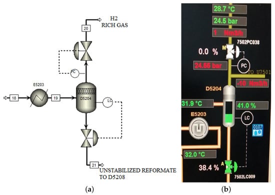
Figure 2.
DRUM D5204 schematic diagram: (a) schematic diagram; (b) graphical user interface (GUI).
3. Mathematical Model
3.1. RD 5204 Mathematical Model
Figure 3 shows the RD5204 (flash drum or separator) which has the following specifications [7]:
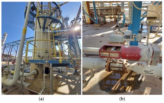
Figure 3.
D5204 in Basrah Refinery: (a) process tank; (b) electrival valve.
- Item: 7502-D5204.
- The mixture is readily accessible at (45) C, (25) bar.
- The gravity 759 kg/m and molar inlet is 48,141 kg/h or (1159.01) kmole/h (constant pressure).
- With pressure (25), this stream will be split into two phases, with 85% liquid and 15% vapor.
- The physical separation is occurring in a flash drum with a height is 5.2 m and a diameter is 1.6 m.
- In the flash drum, liquid–vapor equilibrium is achieved because the relative volatility of the liquids is sufficiently different.
To assist in the conservation of all processing systems (PS), each (PS) should have a unit comprehensive mass balance, one component of mass balance, and a comprehensive energy balance. Momentum balancing is used when there are large pressure or density differences. The dynamics balance equations (DBE) propose that each balance is initially dynamic. The static characteristic of a process may be transformed into a static equation. The flash process establishes the mass and energy balance [9].
- Balance over Total PS:
- –
- Total mass balance:where M is the total mass, is the current mass flow i, subscript V is the vapor, and L is the liquid in multiphase currents.
- –
- Energy balance:with as the heat flow and as the work flow of the system, and () is the specific enthalpy of current , the total energy of total PS.
- Balance over Liquid Process System (PS liquid):
- –
- Total mass balance:with as the liquid level in the tank, as the phase density i (vapor or liquid), and r is the tank radius.
- Balance over Vapor Process System (PS vapor):
- –
- Total mass balance:
where P is the pressure of the vapor phase inside the tank, R is the universal gas constant and the operating temperature, is the molecular mass of vapor, and is the volume of vapor phase inside the flash tank.For liquid or vapor flow through the output flash tank valve, it is necessary to calculate () and (), and the vapor and liquid flows exiting the flash tank arewhere is the coefficient of the valve for phase i, is the valve opening percentage, and is the pressure drop through the valve acting over phase i. In valve sizing, is taken equal to 50% for a nominal or design flow.
3.2. Auto-Tuning PID Mathematical Model
In an ideal PID form, the output u(t) is the sum of the three proportional terms: (P) term, integral (I) term, and derivative (D) term [7].
where is the feedback error, and is the derivative control gain. The transfer function is
The controller’s output is adjusted based on the amount of the mistake using the P action (mode). In certain cases, the steady-state offset can be eliminated with I action (mode), but the D action (mode) forecasts the future trend (mode). A wide range of process applications may benefit from these useful capabilities, and the features’ openness ensures widespread user acceptability [34].
Two estimated frequency responses were evaluated from the relay testing data, which are the fundamental frequency , and . In the case of the system having no disturbance, was selected as , otherwise, . The transfer function of the ideal PID will be as:
where , , and . To design a high-performance PID controller, the optimal parameters of , , and are evaluated based on the estimated frequency response.
We adjust the PID gains automatically in real time in response to the predicted plant frequency response in a closed-loop experiment. We utilize the frequency response estimator to obtain a real-time estimate of a physical plant’s frequency response based on experiments.
- At the normal operating range, we inject sine wave test signals into the plant.
- We collect data on the reaction of the plant’s performance.
- We estimate the frequency.
A recursive least squares (RLS) algorithm [35,36,37,38] is used to evaluate the predicted frequency response. The plant’s frequency response was assumed; when the system is excited by a signal , the steady-state of system response is , as follows:
For any time, and are known. So, they can be employed as regresses in an RLS algorithm to predict and based on system output in real time.
In the case of the excitation signal containing an accumulation of multiple signals, then
The estimation algorithm uses and as regressors to estimate and . For N frequencies, the algorithm uses 2N regresses. The calculation is performed on the assumption that a system with zero nominal input and output is feeding by perturbation signal u(t).
3.3. The Twin-Delayed Deep Deterministic Policy Gradient (TD3) Algorithm
The TD3 algorithm is a technique for off-policy reinforcement learning that is online and model-free. The TD3 agent is an RL agent that incorporates actor–critic skills and pursues the optimal policy that maximizes the expected cumulative long-term reward [39]. The TD3 algorithm is an elongation of the DDPG algorithm. DDPG agents can overvalue functions, which can produce suboptimal policies. To avoid overestimation of the value function, the TD3 method incorporates the following adjustments to the DDPG algorithm.
- The TD3 agent learns two Q-value functions and changes policies based on the estimated minimum value function.
- In contrast to Q functions, TD3 agents modify their policies and targets more slowly.
- When the policy is updated, a TD3 agent introduces noise into the target action, making it less likely to exploit actions with high Q-value estimations.
TD3 agents use the following actor and critic representations.
Critic: One or more Q-value function critics Q (S, A).
Actor: Deterministic policy actor (S).
The following training procedure is used by TD3 agents in which they update their actor and critic models at each time step.
- Initialize each critic Qk(S, A) with random parameter values , and initialize each target critic with the same random parameter values: .
- Initialize the actor with random parameter values , and initialize the target actor with the same parameter values: .
For each time phase of training,
- For the current monitoring S, select action , where N denotes stochastic noise as defined by the noise model.
- Run action A. Observe the benefit R and next monitoring S’.
- Store the knowledge () in the knowledge buffer.
- Sample a random mini-batch of M knowledge () from the knowledge buffer.
- If is a terminal state, set the value function target to . Otherwise, set it to
To compute the cumulative benefit, the agent first computes the next action by passing the next monitoring from the sampled knowledge to the target actor. The agent finds the cumulative rewards by passing the next action to the target critics.
- Update the parameters of each critic at each time training step by minimizing the loss over all sampled experiences.
- At every D1 step, update the actor parameters using the following sampled policy gradient to maximize the expected discounted reward.where A =where is the gradient of the minimum critic output with respect to the action computed by the actor network, and is the gradient of the actor output with respect to the actor parameters. Both gradients are evaluated for observation .
- At every D2 step, update the target actor and critics based on the technique used to update the target.
4. Experiments and Results
This section focuses on validating the D5204 system using MATLAB, as well as the simulation of the real industrial system by designing several experiments. Therefore, the first group of experiments evaluates the performance of the closed-loop system by using a PI controller, and then an auto-tuner is used to optimize the performance of the system; finally, we validate the use of RL to optimize the PI controller for the best performance. The second group of experiments uses the RL agent as an online tuner to optimize the PI parameters; in this case, the RL system works as an RL PI-like controller of RD5204. The D5204 system that is designed by Simulink is shown in Figure 4, and the real parameters of the D5204 system in the process unit of the Basrah Refinery are listed in Table 1 [7].
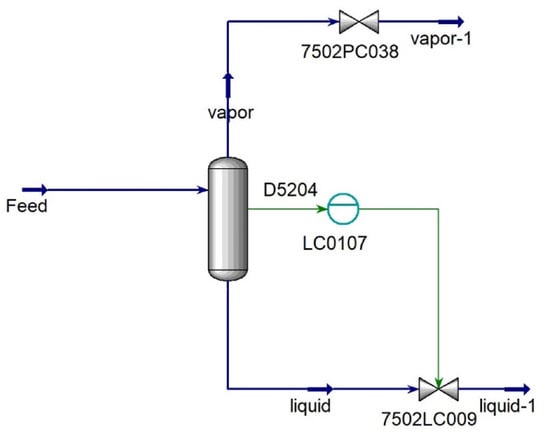
Figure 4.
Graphical representation of model.

Table 1.
Parameters of the D5204 system in process unit of Basrah Refinery.
Several scenarios were designed using Simulink in MATLAB to validate the proposed systems as follows:
- Analyzing the performance of the D5204 system with a PI controller in which the PI parameters are manually tuned in the case of effect factors (inlet feed and opening valve);
- Analyzing the performance of the D5204 system with a PI controller in which the PI parameters are optimized by an auto-tuner in the case of effect factors (inlet feed and opening valve);
- Analyzing the performance of the D5204 system with a PI controller in which the PI parameters are optimized by the RL approach in the case of effect factors (inlet feed and opening valve);
- Using an RL controller as a PI-like controller and analyzing the performance of the D5204 system in the case of effect factors (inlet feed and opening valve).
4.1. PI Controller (Evaluating PI Parameters by Manual Tuning) [7]
The system performance was enhanced by a PI controller, and it will be built in the manner seen in Figure 5. It is being developed at present to enhance the performance with this controller configuration. The settings for the PI will be determined by a trial and error method. This approach is widely used in practically every industrial application and has a high rate of success. There are many challenges, including having an expert and professional engineer available to observe the system’s performance to tune the PI parameters by trial and error. Normally, this mission takes about 4 to 6 work hours to achieve an acceptable system response as that in Basrah Refinery which is shown in Figure 6.

Figure 5.
Overall system with PI control.
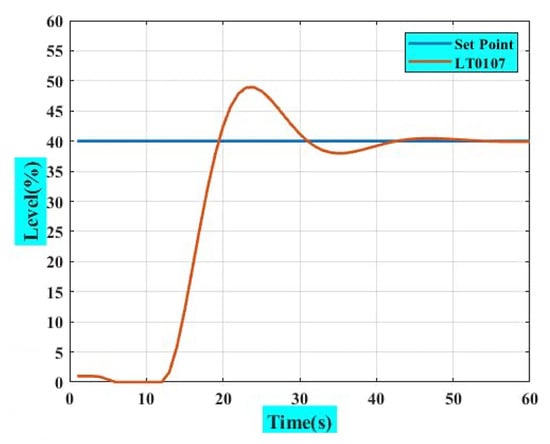
Figure 6.
System response with manual tuning.
Rising-time and overshoot are the most critical components to examine when assessing the system’s reaction and may be used to evaluate the system’s overall performance, since the results indicate a high value for overshoot and other system characteristics. Certain issues arise often in refineries and other industries for a variety of reasons, including insufficient input supplies, valve failures, and so on. Due to this immediate failure happening while the system is running, the situational feed rate will decrease to 250 kg/h causing the level to deviate from the desired level, preventing the system from meeting the performance requirements for the desired process operation—as a result, affecting all product specifications. Another factor influencing system performance is the accuracy of the output control valve. Hence, any modification or failure in this component would decrease the system responsiveness. The result is shown in Figure 7 and Table 2, which show that the system responds to disturbances, such as changing the input feed m2 or opening the valve value and recording the system’s response to these changes after modifying the PI controller.
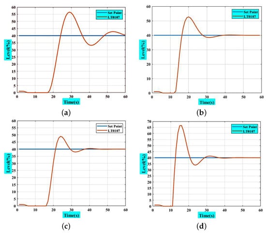
Figure 7.
System response in case of several values of m2 and yi: (a) decrease m2 to 250 kmole/h; (b) increase m2 to 1000 kmole/h; (c) increase yi to 100%; (d) decrease yi to 0%.
Table 2.
Step-response characteristics for system in Figure 7.
4.2. PI Controller (Estimating PI Parameters by Auto-Tuning) [7]
The system in Figure 5 was modified to include the closed-loop PID auto-tuner block, which is added between the PI controller and the plant to optimize the PI parameters, as illustrated in Figure 8. The closed-loop PID auto-tuner blocks functions are equivalent to a unity gain block, except that the u signal is wired directly to u + u. To configure the closed-loop PID auto-tuner block, the following settings should be implemented.
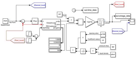
Figure 8.
Overall system with closed-loop PID auto-tuning.
Target bandwidth: Determines the rate at which the controller should reply. The target bandwidth is roughly (2/desired rise time). For a 4 s rising time, set the target bandwidth = 0.5 rad/s.
Target phase margin: Determines the controller’s robustness. Begin with the default setting of 75 degrees in this example.
Experiment sample time: Sample time for the experiment performed by the auto-tuner block. Use the recommended (0.02/bandwidth) for sample time = 0.04 s.
The experiment is started at 140 s to ensure that the material level has reached steady state H = 40. The recommended experiment duration is 200/bandwidth seconds = 200/0.4 = 500 s. With a start time of 140 s, the stop time is 640 s. The simulation stop time is further increased to capture the full experiment. For estimated PI gains, the PID auto-tuning block will employ several approaches, such as insinuating signals into the system to obtain a frequency response in real time. The overall system will be perturbed by a sinusoidal type of testing signal. After finishing the experiment, it is easy to obtain a PI parameter based on plant frequency estimation. The PI controller directly updates the values of the PI parameters. In order to obtain the best system response values, we must first compute the system response characteristic as below.
With a maximum of 60 s needed for system frequency estimation and PI gain values for optimum PI parameters, this tuning strategy has the significant advantage of taking less time to calculate the ideal PI parameters and improving other characteristics, such as the rising time and overshoot, which are shown in Figure 9. Validation of the control system with the same disturbance in the previous scenario was achieved, in which the behavior of the system is shown in Figure 10 and Table 3. From the results, it can be seen that the performance when using the auto-tuning method is superior to the manual tuning of the PI parameters.
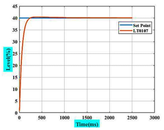
Figure 9.
System response with closed-loop PID auto-tuning.
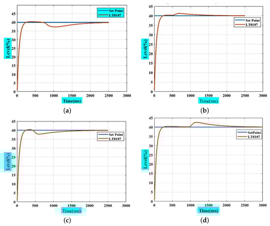
Figure 10.
Response of system with closed-loop auto-tuning PID controller in the case of several values of m2 and yi; (a) decrease m2 to 250 kmole/h; (b) increase m2 to 1000 kmole/h; (c) increase yi to 100%; (d) decrease yi to 0%.
Table 3.
Step-response characteristics for system in Figure 10.
4.3. PI Controller (Estimating PI Parameters by RL Approach)
In this section, the improvement of a PI controller using the RL approach (TD3) was considered. When comparing model-free RL with other techniques, model-based tuning strategies may provide acceptable results with a reduced tuning time for relatively simple control tasks involving only one or a few tunable parameters. RL techniques, on the other hand, may be more appropriate for highly non-linear systems or adaptive controller tuning. The system in Figure 5 was modified by using an RL block for the estimation of PI parameters via the following steps:
- Delete the PI controller.
- Insert an RL agent block.
- Create the observation vector , where is the height of the tank, and r is the reference height. Connect the observation signal to the RL agent block.
- Define the reward function for the RL agent as the negative, i.e.,
The RL agent maximizes this reward, for which the resulting model is as shown in Figure 11.
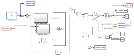
Figure 11.
System with RL agent.
4.3.1. Create TD3 Agent
When we wish to create a TD3 agent that is given observations, a TD3 agent selects the action to perform using an actor. To build the actor, we first establish a deep neural network using the observation input and the action output. A PI controller can be modeled as a neural network (NN) with one fully connected layer with error and error integral observations: . Here:
- U is the outlet of the actor NN.
- and are the absolute values of the neural network weights.
- is the height of the tank, and r is the reference height.
Using two critic value–function representations, a TD3 proxy approximates the long-term award associated with monitoring and actions. To begin, we construct a deep neural network with two inputs, observation and action, and a single output. We configure the agent using the following options:
- Set the agent to use the controller sample time Ts;
- Set the mini-batch size to 128 experience samples;
- Set the experience buffer length to ;
- Set the exploration model and target policy smoothing model to use Gaussian noise with variance of 0.1.
4.3.2. Train Agent
To train the agent, first set the following:
- Run each training step for at most 1000 episodes, with every episode enduring at most 100 schedule steps.
- Show the training headway in the episode manager (set the plots option) and consult the command-line display.
- Stop training when the agent receives an average cumulative reward greater than −200 over 100 consecutive episodes.
- At this point, the agent can control the level in the tank.
Finally, the optimal PI parameters can be evaluated, which are and . The parameters of the PI controller block shown in Figure 5 will be set by using the optimal parameters evaluated by RL. Therefore, the step response characteristics will be as shown in Figure 12.
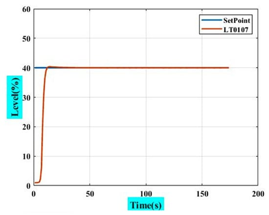
Figure 12.
System response after tuning by RL.
Figure 13 and Table 4 show a system response in the case of disturbances. Different methods of disruption are included, such as increasing or decreasing the input feed (m2) and increasing or decreasing the opening valve (yi). After testing the system in the case of optimizing the PI parameters using the RL approach, the results reveal the good performance of the proposed system.
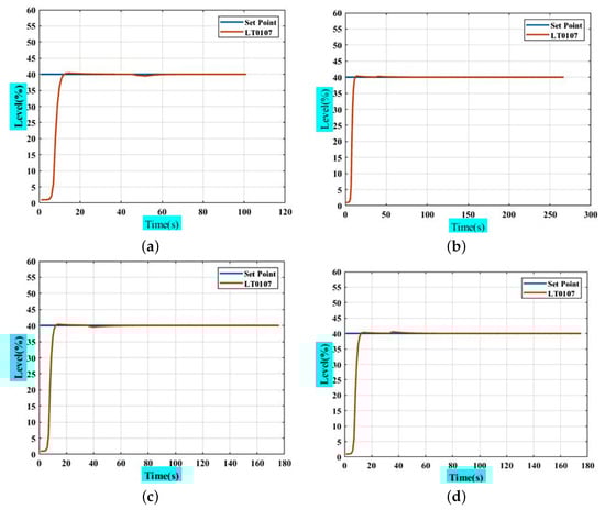
Figure 13.
Response of system with reinforcement learning for optimization of PI in case of several values of m2 and yi: (a) decrease m2 to 250 kmole/h; (b) increase m2 to 1000 kmole/h; (c) decrease yi to 100%; (d) decrease yi to 0%.
Table 4.
Step-response characteristics for system in Figure 13.
4.4. RL Agent as PI-like Controller
The objective of this part is to show how we can use RL as an online tuner to optimize the PI parameters; in this case, the RL system is working as an RL PI-like controller of RD5204, as shown in Figure 11, and we study the performance of the proposed system, which is shown in Figure 14. Further, the system was validated under the same condition as in previous scenarios; after applying disturbances, the response of the system is as shown in Figure 15 and Table 5. Although the system response seems similar to that in the previous setup (optimization of PI by using RL), there is an important difference. In scenario three, we obtain fixed parameters for the PI controller, but, in the case of using RL as a PI-Like controller, the agent will still learn online with a long period of system operation, which will offer the system more reliability and experience.
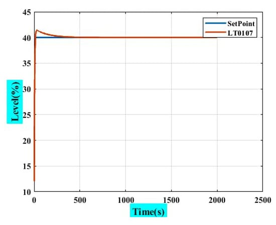
Figure 14.
System response after being controlled by RL agent.
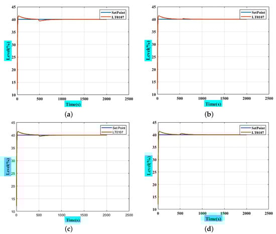
Figure 15.
Response of system with reinforcement learning as controller in the case of several values of m2 and yi: (a) decrease m2 to 250 kmole/h; (b) increase m2 to 1000 kmole/h; (c) increase yi to 100%; (d) decrease yi to 0%.
Table 5.
Step-response characteristics for system in Figure 15.
4.5. Comparison of Use of RL as an Offline Tuner and PI-like Controller
To compare the performance of RL as an online and offline tuner, RL is used as a particular optimization element for the PI controller and as a controller itself, which is known as the PI-like controller. To show that there is a large difference between these two methods, the system performance was tested in the case of using these controllers under the same conditions.
To achieve the mentioned comparison, the process noise was added to the system; this process noise was represented by the band-limited white noise block. Process noise exists in the real world and is manifested in various forms as a result of certain causes, such as physical aspects of electronic circuits, wires, or electrical and magnetic causes as a result of external influences on the signal, which in turn affects the overall operation of the system.
Figure 16 shows the performance of the PI controller in the case of using RL for offline parameter tuning and RL as a PI-like controller, in which the performance when using the RL as a PI-like controller is superior to the other method. In this figure, we show that the case of using RL as an offline tuner leads to the use of the conventional PI controller for process operation; therefore, there is no prediction for stochastic behavior, and the system will not overcome the external noise. Meanwhile, in the case of using RL as an online tuner, this leads to the use of RL as a PI-like controller during the operation of the process; therefore, the RL will optimize the PI parameters based on the prediction of the performance of the system in the future to improve the performance of the system. From this discussion, it can be concluded that the use of RL as a PI-like controller is more resistant to external noise.
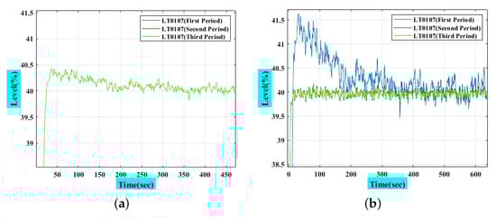
Figure 16.
System response under process noise for two approaches (online and offline tuning): (a) offline tuning with process noise; (b) online tuning with process noise.
Here, it is vital to identify the strengths and weaknesses of each method; therefore, each method may be introduced based on the controlled application requirement.
- The values extracted from the offline tuner are fixed for a conventional PI controller during operation, but the values that are evaluated by the online tuner are changeable and improved during operation; therefore, it is more resistant to external noise due to continuous learning, improvement, exploration, and event anticipation.
- Due to the additional complexity of the online tuner, the offline tuner has a faster reaction time than its online counterpart.
- In the case of offline training, the duration of training is less than that of online training; thus, the best option is determined based on the requirements.
- In certain industrial applications that require an auto-stop, the system’s reaction speed is necessary; therefore, the online tuner is unsuitable in comparison to the offline case.
- Economically, the offline tuner is more costly than the online tuner due to the increase in complexity and, thus, the need for more devices and capabilities, particularly in applications with a large number of control paths.
In addition, Table 6 illustrates the performance of the system with RL in the two methods, as a control and an optimization method. Some differences should be highlighted, such as the fact that the time of rising in the case of the online tuner is longer than in the case of the offline tuner, and this is therefore reflected in the stability of the system and its ability to reach a stable state, but this factor has no impact on the RD5204 application of the refinery. Further, the offline tuner is superior in terms of overshoot and settling values. These differences are considered acceptable due to the different nature of the internal formation of both the PI controller and the agent in RL, as the principal operation of RL is dependent on exploration and exploitation, which leads to approximation. However, the task of reinforcement learning as a controller remains the greatest in terms of the ability to modify the overall performance of the system throughout each operation.
Table 6.
Step-response characteristics for systems in Figure 16.
5. Conclusions
This paper focused on using the RL approach for the level control of the separator drum unit in a refinery system in which the mathematical model of Drum RD5204 is derived to study the response of the system. A PI controller is proposed to improve the system’s response, in which the PI parameters are manually calculated. From the results, the system’s response was superior to that of the conventional controller, but it did not achieve the required performance. In the case of using the auto-tuning method for PI parameter evaluation, the response is superior to the manual tuning method, where the system performance was significantly improved, and it is more reliable and robust against disturbances. The employment of reinforcement learning (RL) as an offline tuner leads to an enhancement in the system’s performance and the system’s ability to resist interruptions and unexpected changes, as well as return to a stable state. Utilizing the RL agent as an online tuner for the PI parameters, in which the online tuner values are adaptable during the operation, makes it more resistant to external noise as a result of continuous learning, exploration, and event anticipation. The validation of the system controller that uses online and offline reinforcement learning techniques for optimization against process noise showed that online tuning was able to attenuate the process noise and reduce it after certain operational periods, while its value was still constant in the case of using offline tuning; therefore, this is an advantage in favor of online tuners.
Author Contributions
Methodology, A.A.A. and M.T.R.; Validation, B.N.A.; Formal analysis, A.A.A. and M.T.R.; Investigation, A.A.A., M.T.R. and B.N.A.; Resources, V.B. and P.M.; Data curation, B.N.A.; Writing—original draft, A.A.A. and M.T.R.; Writing—review & editing, V.B. and P.M.; Project administration, V.B.; Funding acquisition, P.M. All authors have read and agreed to the published version of the manuscript.
Funding
This work has received no external funding.
Acknowledgments
The research was partially supported by the FIM UHK specific research project 2107 Integration of Departmental Research Activities and Students’ Research Activities Support III. The authors also express their gratitude to Patrik Urbanik for his assistance and helpfulness.
Conflicts of Interest
The authors have no conflicts of interest relevant to this article.
References
- Chirita, D.; Florescu, A.; Florea, B.C.; Ene, R.; Stoichescu, D.A. Liquid level control for industrial three tanks system based on sliding mode control. Rev. Roum. Sci. Technol. Électrotechnol. Énerg. 2015, 60, 437–446. [Google Scholar]
- Dorf, R.C.; Bishop, R.H. Modern Control Systems; Prentice-Hall: Englewood Cliffs, NJ, USA, 2004. [Google Scholar]
- Liptak, B.G. Instrument Engineers, Volume Two: Process Control and Optimization; CRC Press: Boca Raton, FL, USA, 2018. [Google Scholar]
- Smith, R.S.; Doylel, J. The Two Tank Experiment: A Benchmark Control Problem. In Proceedings of the American Control Conference, Milwaukee, WI, USA, 27–29 June 2018. [Google Scholar]
- Zhao, Z.; Zhang, X.; Li, Z. Tank-Level Control of Liquefied Natural Gas Carrier Based on Gaussian Function Nonlinear Decoration. J. Mar. Sci. Eng. 2020, 8, 695. [Google Scholar] [CrossRef]
- Short, M.; Selvakumar, A.A. Non-Linear Tank Level Control for Industrial Applications. Appl. Math. 2020, 11, 876. [Google Scholar] [CrossRef]
- Ali, A.A.; Rashid, M.T. Design PI Controller for Tank Level in Industrial Process. Iraqi J. Electr. Electron. Eng. 2022, 18, 82–92. [Google Scholar] [CrossRef]
- Ademola, O.; Akpa, J.; Dagde, K. Modeling and Simulation of Two-Staged Separation Process for an Onshore Early Production Facility. Adv. Chem. Eng. Sci. 2019, 9, 127. [Google Scholar] [CrossRef]
- Mokhatab, S.; Poe, W.A. Handbook of Natural Gas Transmission and Processing; Gulf Professional Publishing: Houston, TX, USA, 2012. [Google Scholar]
- Keidy, R.; Morales, L.; Alvarez, H. Flash distillation modeling and a multiloop control proposal. In Proceedings of the IEEE 2nd Colombian Conference on Automatic Control (CCAC), Manizales, Colombia, 14–16 October 2015. [Google Scholar]
- Seames, W. Designing Controls for the Process Industries; CRC Press: Boca Raton, FL, USA, 2017. [Google Scholar]
- Marlin, T.E. Process Control; McGraw-Hill International Editions: New York, NY, USA, 2018. [Google Scholar]
- Zhang, Z.; Wu, Z.; Dur, H.; Albalawi, F.; Christofides, P.D. On integration of feedback control and safety systems: Analyzing two chemical process applications. Int. J. Control. Autom. Syst. 2020, 132, 616–626. [Google Scholar] [CrossRef]
- Xu, J.; Shao, H. A novel method of PID tuning for integrating processes. In Proceedings of the 42nd IEEE International Conference on Decision and Control, Maui, HI, USA, 9–12 December 2004. [Google Scholar]
- Bucz, Š.; Kozáková, A. Advanced methods of PID controller tuning for specified performance. In PID Control for Industrial Processes; InTech Open: London, UK, 2018; pp. 73–119. [Google Scholar]
- Chidambaram, M.; Saxena, N. Relay Tuning of PID Controllers; Springer: Tamil Nadu, India, 2018. [Google Scholar]
- Pandey, S.K.; Veeranna, K.; Kumai, B.; Deshmukh, K.U. A Robust Auto-tuning Scheme for PID Controllers. In Proceedings of the 46th Annual Conference of the IEEE Industrial Electronics Society, Singapore, 18–21 October 2020. [Google Scholar]
- Vilanova, R.; Arrieta, O.; Ponsa, P. Robust PI/PID controllers for load disturbance based on direct synthesis. ISA Trans. 2018, 81, 177–196. [Google Scholar] [CrossRef] [PubMed]
- Singh, A.P.; Mukherjee, S.; Nikolaou, M. Debottlenecking level control for tanks in series. J. Process. Control. 2014, 24, 158–171. [Google Scholar] [CrossRef]
- Jáuregui, C.; Duarte-Mermoud, M.A.; Oróstica, R.; Travieso-Torres, J.C.; Beytía, O. Conical tank level control using fractional order PID controllers: A simulated and experimental study. Control. Theory Technol. 2016, 14, 369–384. [Google Scholar] [CrossRef]
- Backi, C.J.; Skogestad, S. A simple dynamic gravity separator model for separation efficiency evaluation incorporating level and pressure control. In Proceedings of the American Control Conference (ACC), Seattle, WA, USA, 24–26 May 2017. [Google Scholar]
- Sásig, R.; Naranjo, C.; Pruna, E.; Chicaiza, W.D.; Chicaiza, F.A.; Carvajal, C.P.; Andaluz, V.H. An Implementation on Matlab Software for Non-linear Controller Design Based on Linear Algebra for Quadruple Tank Process. In Proceedings of the World Conference on Information Systems and Technologies, Naples, Italy, 27–29 March 2018. [Google Scholar]
- Reyes-Lúa, A.; Backi, C.J.; Skogestad, S. Improved PI control for a surge tank satisfying level constraints. IFAC-PapersOnLine 2018, 51, 835–840. [Google Scholar] [CrossRef]
- Sathasivam, L.; Elamvazuthi, I.; Ahamed Khan, M.K.A.; Parasuraman, S. Tuning a three-phase separator level controller via particle swarm optimizationalgorithm. In Proceedings of the International Conference on Recent Trends in Electrical, Control and Communication (RTECC), Malaysia, Malaysia, 20–22 March 2018. [Google Scholar]
- Yu, S.; Lu, X.; Zhou, Y.; Feng, Y.; Qu, T.; Chen, H. Liquid level tracking control of three-tank systems. Int. J. Control. Autom. Syst. 2020, 18, 2630–2640. [Google Scholar] [CrossRef]
- Nath, U.M.; Dey, C.; Mudi, R.K. Fuzzy tuned model based control for level and temperature processes. Microsyst. Technol. 2019, 25, 819–827. [Google Scholar] [CrossRef]
- Ye, J.; Zhang, X.; Lv, C.; Wang, P.; Lv, H. Design of liquid level control system for double tank. IOP Conf. Ser. Mater. Sci. Eng. 2020, 740, 012097. [Google Scholar] [CrossRef]
- Nath, U.M.; Dey, C.; Mudi, R.K. Desired characteristic equation based PID controller tuning for lag-dominating processes with real-time realization on level control system. IEEE Control. Syst. Lett. 2020, 5, 1255–1260. [Google Scholar] [CrossRef]
- Singh, V.P.; Patnana, N.; Singh, S. PID controller tuning using hybrid optimisation technique based on Box’s evolutionary optimisation and teacher-learner-based-optimisation. Int. J. Comput. Aided Eng. Technol. 2020, 13, 258–270. [Google Scholar] [CrossRef]
- Kos, T.; Huba, M.; Vrančić, D. Parametric and Nonparametric PID controller tuning method for integrating processes based on Magnitude Optimum. Appl. Sci. 2020, 10, 6012. [Google Scholar] [CrossRef]
- Mary, A.H.; Miry, A.H.; Miry, M.H. ANFIS based reinforcement learning strategy for control a nonlinear coupled tanks system. J. Electr. Eng. Technol. 2022, 17, 1921–1929. [Google Scholar] [CrossRef]
- Ziegler, J.G.; Nichols, N.B. Optimum settings for automatic controllers. J. Dyn. Syst. Meas. Control. 1993, 115, 759–765. [Google Scholar] [CrossRef]
- Available online: http://www.src.gov.iq/en/about_us (accessed on 15 March 2023).
- McDonald, K.A.; McAvoy, T.J. Decoupling Dual Composition Controllers 1. Steady State Results. In Proceedings of the American Control Conference, San Francisco, CA, USA, 22–24 June 1983. [Google Scholar]
- Davis, M.; Vinter, R. Minimum-Variance and Self-Tuning Control. In Stochastic Modelling and Control; Springer: Berlin/Heidelberg, Germany, 1985. [Google Scholar]
- Haykin, S. Recursive least squares adaptive filters. In Adaptive Filter Theory; Pearson Education India: Delhi, India, 2002; pp. 436–447. [Google Scholar]
- Monson, H.H. Recursive Least Squares. Statistical Digital Signal Processing and Modelling; Wiley: Hoboken, NJ, USA, 1996. [Google Scholar]
- Available online: https://en.wikipedia.org/w/index.php?title=Recursive_least_squares_filter&oldid=1059014247 (accessed on 20 February 2023).
- Scott, F.; Hoof, H.; Meger, D. Addressing function approximation error in actor-critic methods. In Proceedings of the International Conference on Machine Learning, Stockholm, Sweden, 10–15 July 2018. [Google Scholar]
Disclaimer/Publisher’s Note: The statements, opinions and data contained in all publications are solely those of the individual author(s) and contributor(s) and not of MDPI and/or the editor(s). MDPI and/or the editor(s) disclaim responsibility for any injury to people or property resulting from any ideas, methods, instructions or products referred to in the content. |
© 2023 by the authors. Licensee MDPI, Basel, Switzerland. This article is an open access article distributed under the terms and conditions of the Creative Commons Attribution (CC BY) license (https://creativecommons.org/licenses/by/4.0/).