

Levy Flight-Based Improved Grey Wolf Optimization: A Solution for Various Engineering Problems

 ,
,  and
and 
Abstract
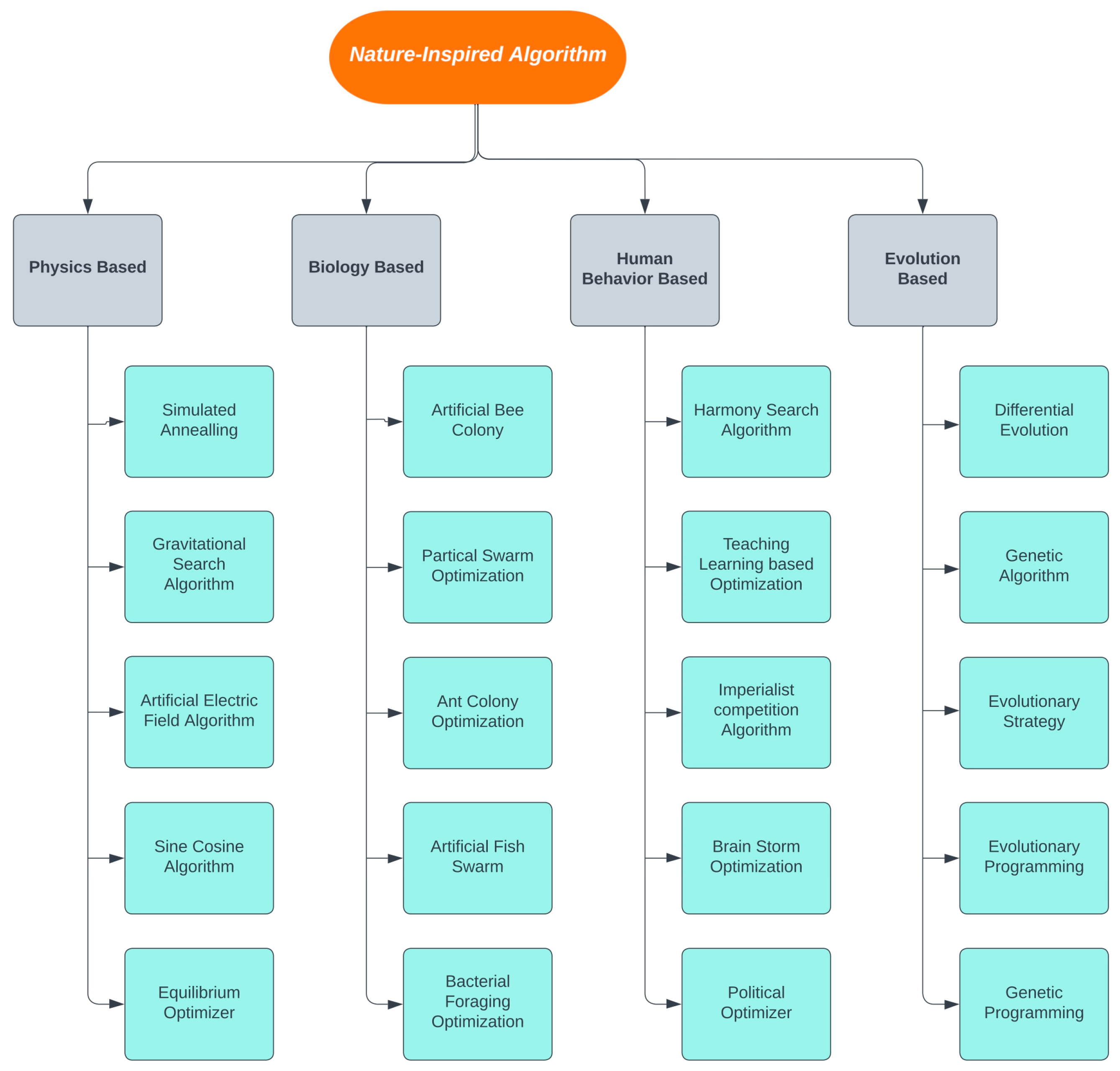
1. Introduction
- Engineering: Metaheuristic algorithms are used in engineering to optimize the design of structures, such as bridges and buildings.
- Computer science: Metaheuristic algorithms are used in computer science to optimize the performance of the algorithms and systems, such as scheduling and routing.
- Operations research: Metaheuristic algorithms are used in operations research to solve problems in areas such as logistics and supply chain management.
2. Optimization
- Mathematical programming: These techniques are based on the use of mathematical models to represent the problem and constraints. The solution is then found by solving the mathematical equations.
- Gradient-based methods: These techniques are based on the use of gradients, which are the directions of the steepest ascent or descent. The solution is found by moving in the direction of the gradient until a local or global optimum is reached.
- Metaheuristic algorithm: These techniques are based on the use of metaheuristics, which are rules of thumb, to guide the search for a solution. The solution is found by iteratively improving an initial solution over time.
3. Optimization Algorithm and New Proposed Algorithms
3.1. Grey Wolf Optimization
| Algorithm 1 GWO Algorithm |
| Form the grey wolf population. Evaluate the accuracy of every response. For each iteration: For every single grey wolf in the population: Generate a new solution. Analyze the new solution’s potential. Update a grey wolf’s location in accordance with the updated solution. Sort the grey wolves based on their fitness. Each grey wolf’s location will be updated dependent on where the other grey wolves in the population are. Return the best solution as the result. |
3.2. Improved Grey Wolf Optimization
| Algorithm 2 IGWO Algorithms |
Set the grey wolf population (solutions). Evaluate the accuracy of every response. Arrange solutions in decreasing fitness order. Make the best response the dominant α wolf. Make the second best response the β wolf. Make the third best response the δ wolf. For each iteration: Generate new solutions for each grey wolf. Examine the appropriateness of each new solution. According to the new answer, adjust each grey wolf’s location. Based on a combination of the α wolf’s answer, the β wolf’s solution, and the δ wolf’s solution, the α wolf’s location should be updated. Using the α wolf’s location and their solutions, adjust the positions of the wolves. Evaluate the fitness of the updated solutions. Arrange the grey wolves according to their most recent fitness. Update the 𝑎, 𝛽, and δ wolves based on the new sorting. Return the best solution (the alpha wolf) as the result. |
3.3. Levy Flight Improved Grey Wolf Optimization
- μ is the parameter for location (the mean of the distribution);
- σ is a scale parameter (the standard deviation of the distribution);
- γ is the tail index parameter (controls the shape of the distribution).
| Algorithm 3 Newly Proposed |
| Set the grey wolf population (solutions). Evaluate the accuracy of every response. Arrange solutions in decreasing fitness order. Make the best response the dominant α wolf. Make the second best response the β wolf. Make the third best response the δ wolf. Evaluate the new position of the wolves and update it with the initial position. For each iteration: Generate new solutions for each grey wolf using Levy flight. Evaluate the accuracy of every new solution. According to the new answer, adjust each grey wolf’s location. The 𝛼 wolf’s location is updated based on a combination of its solution and the solutions of the 𝛽 and 𝛿 wolves. Based on a combination of the α wolf’s answer, the β wolf’s solution, and the δ wolf’s solution, the α wolf’s location should be updated. Evaluate the fitness of the updated solutions. Arrange the grey wolves according to their most recent fitness. Update the 𝛼, 𝛽, and 𝛿 wolves based on the new sorting. Return the best solution (the 𝛼 wolf) as the result. |
4. Results and Discussion
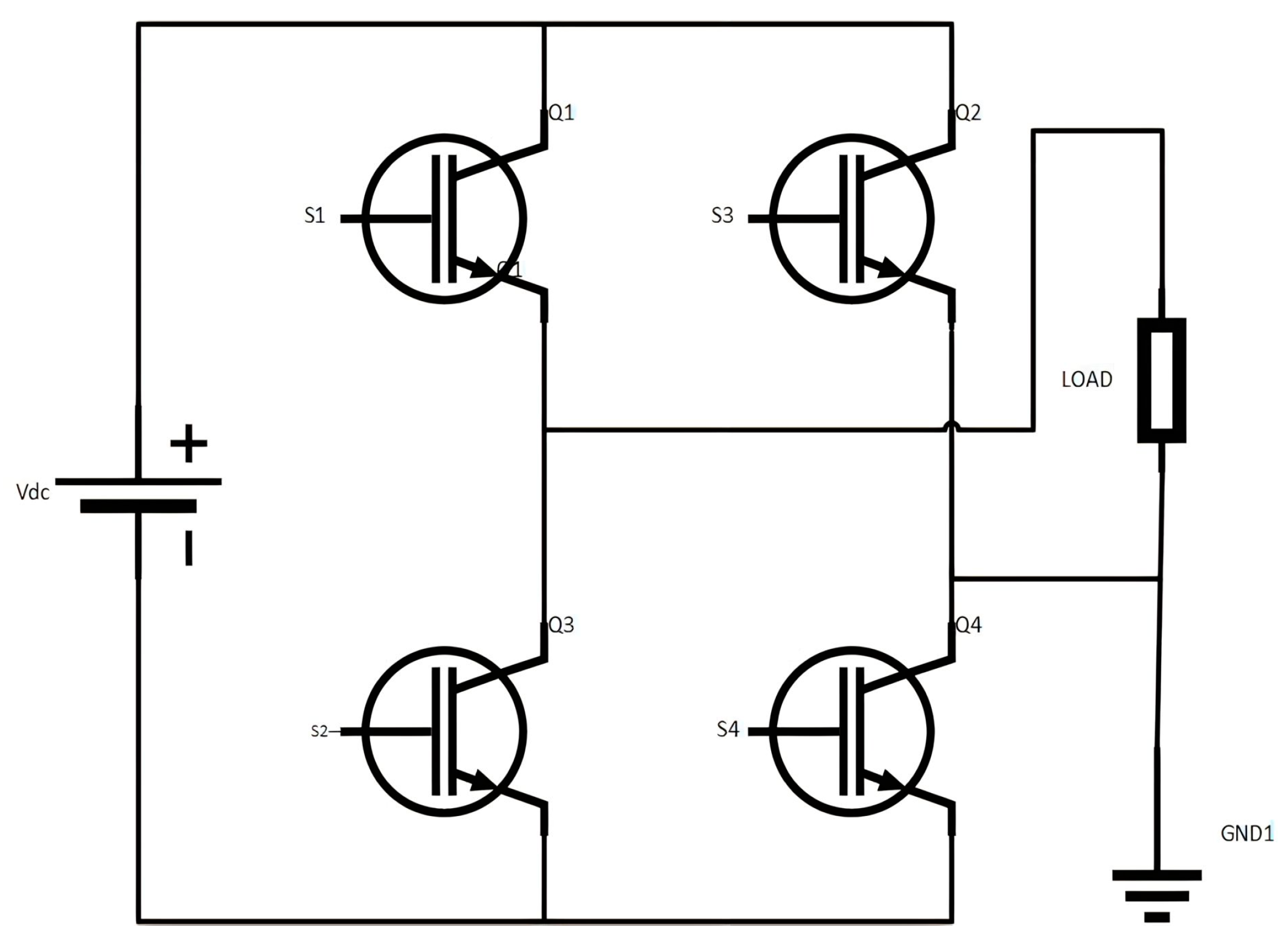
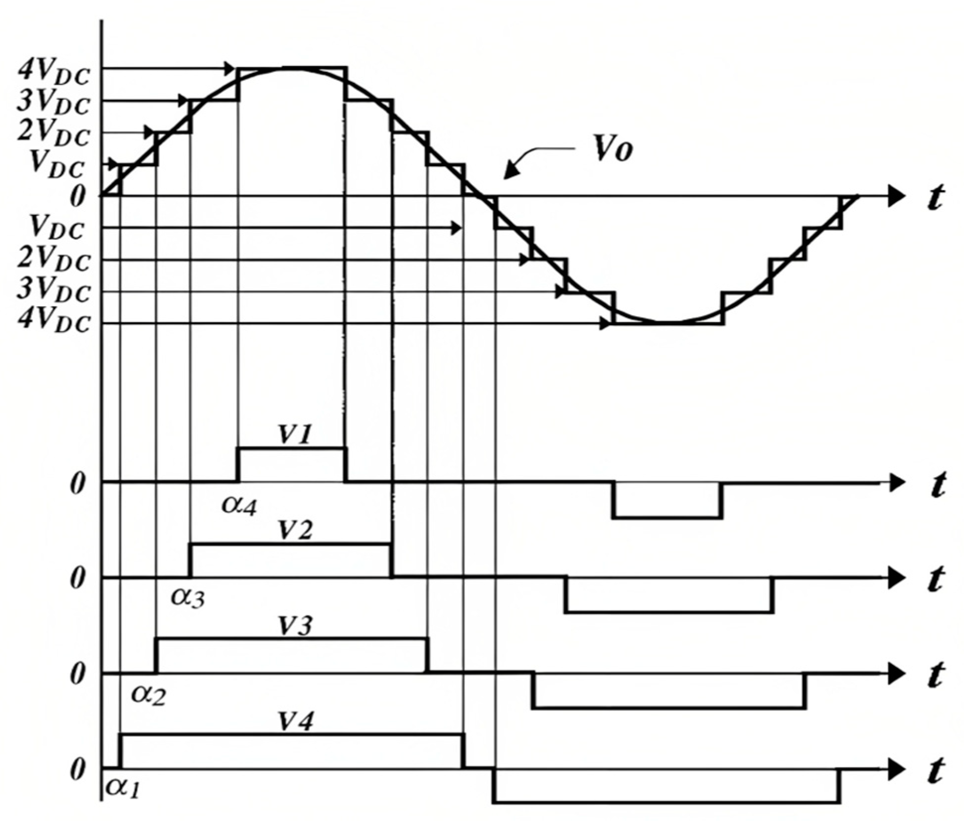
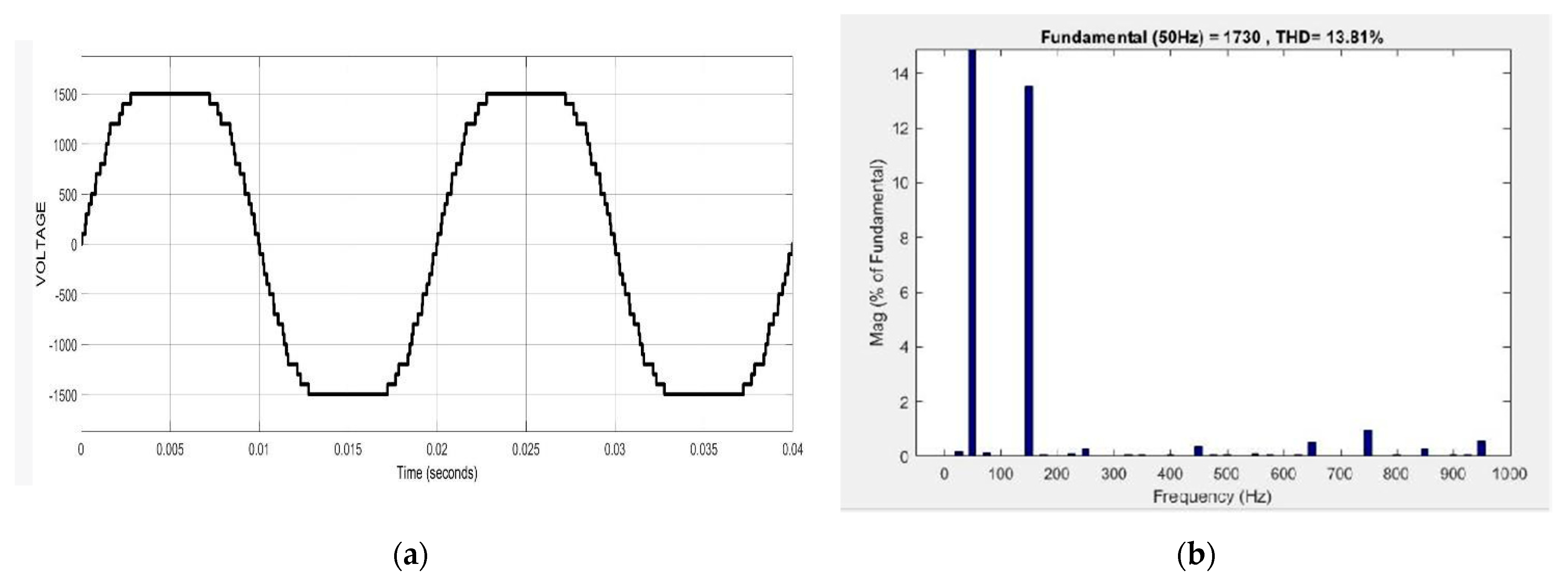
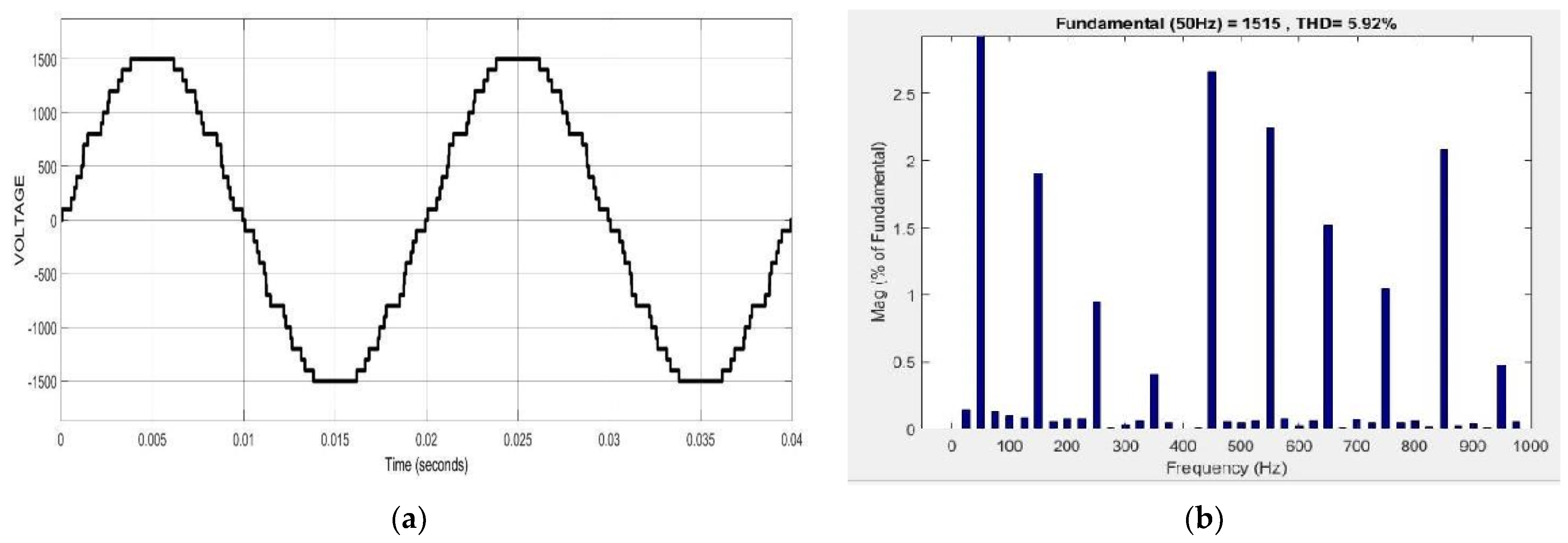
4.1. 31-Level Cascaded H-Bridge MLI
- is the output voltage waveform;
- is the resulting waveform’s fundamental frequency;
- is the inverter’s H-bridge module count;
- is the DC voltage input of the kth H-bridge module.
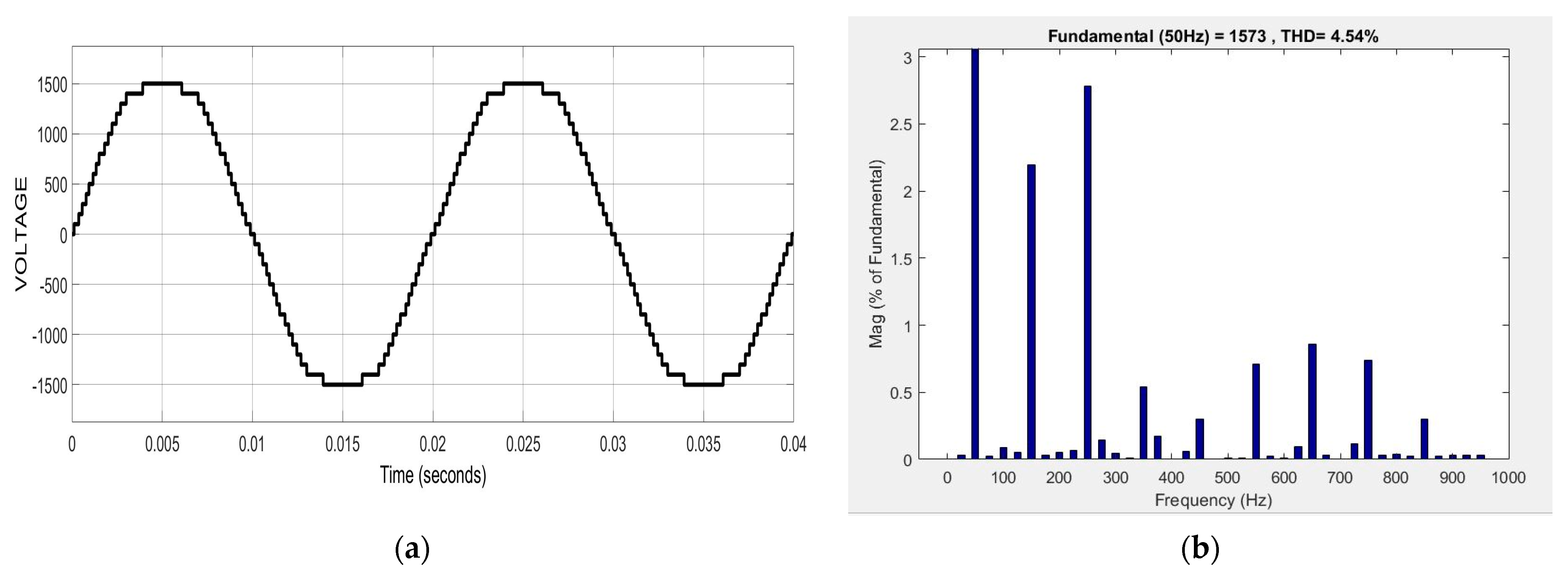
4.2. Harmonics
- Increased current levels: Harmonics can cause an increase in the RMS current levels, which can result in the overloading of conductors, transformers, and other electrical equipment.
- Decreased power factor: A reduction in the power factor, a measurement of an electrical system’s efficiency, can be brought on by the presence of harmonics. This can result in increased energy costs and decreased system efficiency.
- Increased heating: The additional current levels caused by harmonics can result in increased heating in conductors and transformers, which can reduce their life expectancy and cause safety issues.
- Interference with communication systems: Harmonics can interfere with communication systems and cause problems such as data corruption and interference with radio and television signals.
4.3. Total Harmonics Distortion
5. Engineering Problems
5.1. Tension Compression Spring
5.2. Pressure Vessel Design
5.3. Welded Beam Design
6. Conclusions
Author Contributions
Funding
Data Availability Statement
Conflicts of Interest
References
- Kaur, K.; Kumar, Y. Swarm Intelligence and its applications towards Various Computing: A Systematic Review. In Proceedings of the 2020 International Conference on Intelligent Engineering and Management (ICIEM), London, UK, 17–19 June 2020; pp. 57–62. [Google Scholar] [CrossRef]
- Trianni, V.; Tuci, E.; Passino, K.M.; Marshall, J.A.R. Swarm Cognition: An interdisciplinary approach to the study of self-organising biological collectives. Swarm Intell. 2011, 5, 3–18. [Google Scholar] [CrossRef]
- Sneha; Wajahat. Swarm Intelligence. Int. J. Sci. Eng. Res. 2017, 8, 10. [Google Scholar]
- Hazem, A.; Glasgow, J. Swarm Intelligence: Concepts, Models and Applications; School of Computing, Queen’s University: Kingston, ON, Canada, 2012. [Google Scholar] [CrossRef]
- Zahra, B.; Siti Mariyam, S. A review of population-based meta-heuristic algorithm. Int. J. Adv. Soft Comput. Its Appl. 2013, 5, 1–35. [Google Scholar]
- Colin, R. Genetic Algorithms. In Handbook of Metaheuristics; Springer: Boston, MA, USA, 2010; pp. 109–139. [Google Scholar] [CrossRef]
- Seyedali, M. Particle Swarm Optimisation. In Evolutionary Algorithms and Neural Networks; Springer: Cham, Switzerland, 2019; pp. 15–31. [Google Scholar] [CrossRef]
- Yi, G.; Jin, M.; Zhou, Z. Research on a Novel Ant Colony Optimization Algorithm. In Advances in Neural Networks—Lecture Notes in Computer Science; Zhang, L., Lu, B.L., Kwok, J., Eds.; Springer: Berlin/Heidelberg, Germany, 2010; Volume 6063. [Google Scholar] [CrossRef]
- Storn, R.; Price, K. Differential Evolution—A Simple and Efficient Heuristic for global Optimization over Continuous Spaces. J. Glob. Optim. 1997, 11, 341–359. [Google Scholar] [CrossRef]
- Ribeiro, M.d.R.; Aguiar, M.S.d. Cultural Algorithms: A Study of Concepts and Approaches. In Proceedings of the 2011 Workshop-School on Theoretical Computer Science, Pelotas, Brazil, 24–26 August 2011; pp. 145–148. [Google Scholar] [CrossRef]
- Rutenbar, R.A. Simulated annealing algorithms: An overview. IEEE Circuits Devices Mag. 1989, 5, 19–26. [Google Scholar] [CrossRef]
- Prajapati, V.K.; Jain, M.; Chouhan, L. Tabu Search Algorithm (TSA): A Comprehensive Survey. In Proceedings of the 2020 3rd International Conference on Emerging Technologies in Computer Engineering: Machine Learning and Internet of Things (ICETCE), Jaipur, India, 7–8 February 2020; pp. 1–8. [Google Scholar] [CrossRef]
- Zhang, J.; Zhang, P. A study on harmony search algorithm and applications. In Proceedings of the 2018 Chinese Control and Decision Conference (CCDC), Shenyang, China, 9–11 June 2018; pp. 736–739. [Google Scholar] [CrossRef]
- Kytöjoki, J.; Nuortio, T.; Bräysy, O.; Gendreau, M. An efficient variable neighborhood search heuristic for very large scale vehicle routing problems. Comput. Oper. Res. 2007, 34, 2743–2757. [Google Scholar] [CrossRef]
- Mohammad, H.; Mohammad, H. Simplex method to Optimize Mathematical manipulation. Int. J. Recent Technol. Eng. (IJRTE) 2019, 7, 5. [Google Scholar]
- Alonso, G.; del Valle, E.; Ramirez, J.R. 5—Optimization methods. In Woodhead Publishing Series in Energy, Desalination in Nuclear Power Plants; Woodhead Publishing: Shaxton, UK, 2020; pp. 67–76. ISBN 9780128200216. [Google Scholar] [CrossRef]
- Lian, P.; Wang, C.; Xiang, B.; Shi, Y.; Xue, S. Gradient-based optimization method for producing a contoured beam with single-fed reflector antenna. J. Syst. Eng. Electron. 2019, 30, 22–29. [Google Scholar] [CrossRef]
- Wolpert, D.H.; Macready, W.G. No free lunch theorems for optimization. IEEE Trans. Evol. Comput. 1997, 1, 67–82. [Google Scholar] [CrossRef]
- Shukla, P.; Singh, S.K.; Khamparia, A.; Goyal, A. Nature-inspired optimization techniques. In Nature-Inspired Optimization Algorithms; Academic Press: Cambridge, MA, USA, 2021. [Google Scholar] [CrossRef]
- Ingber, A.; Lester, I. Simulated annealing: Practice versus theory. Math. Comput. Model. 2002, 18, 29–57. [Google Scholar] [CrossRef]
- Rashedi, E.; Nezamabadi-Pour, H.; Saryazdi, S. GSA: A Gravitational Search Algorithm. Inf. Sci. 2009, 179, 2232–2248. [Google Scholar] [CrossRef]
- Anita; Yadav, A.; Kumar, N. Artificial electric field algorithm for engineering optimization problems. Expert Syst. Appl. 2020, 149, 113308. [Google Scholar] [CrossRef]
- Mirjalili, S. SCA: A Sine Cosine Algorithm for solving optimization problems. Knowl. Based Syst. 2016, 96, 120–133. [Google Scholar] [CrossRef]
- Faramarzi, A.; Heidarinejad, M.; Stephens, B.; Mirjalili, S. Equilibrium optimizer: A novel optimization algorithm. Knowl. Based Syst. 2020, 191, 105190. [Google Scholar] [CrossRef]
- Bansal, J.C.; Sharma, H.; Jadon, S.S. Artificial bee colony algorithm: A survey. Int. J. Adv. Intell. Paradig. 2013, 5, 123–159. [Google Scholar] [CrossRef]
- Neshat, M.; Sepidnam, G.; Sargolzaei, M.; Toosi, A.N. Artificial fish swarm algorithm: A survey of the state-of-the-art, hybridization, combinatorial and indicative applications. Artif. Intell. Rev. 2014, 42, 965–997. [Google Scholar] [CrossRef]
- Guo, C.; Tang, H.; Niu, B.; Lee, C.B.P. A survey of bacterial foraging optimization. Neurocomputing 2021, 452, 728–746. [Google Scholar] [CrossRef]
- Zou, F.; Chen, D.; Xu, Q. A survey of teaching–learning-based optimization. Neurocomputing 2019, 335, 366–383. [Google Scholar] [CrossRef]
- Atashpaz-Gargari, E.; Lucas, C. Imperialist competitive algorithm: An algorithm for optimization inspired by imperialistic competition. In Proceedings of the 2007 IEEE Congress on Evolutionary Computation, Singapore, 25–28 September 2007; pp. 4661–4667. [Google Scholar] [CrossRef]
- Zhang, T.; Yang, C.; Zhao, X. Using Improved Brainstorm Optimization Algorithm for Hardware/Software Partitioning. Appl. Sci. 2019, 9, 866. [Google Scholar] [CrossRef]
- Abdelhamid, M.; Kamel, S.; Mohamed, M.A.; Aljohani, M.; Rahmann, C.; Mosaad, M.I. Political Optimization Algorithm for Optimal Coordination of Directional Overcurrent Relays. In Proceedings of the 2020 IEEE Electric Power and Energy Conference (EPEC), Edmonton, AB, Canada, 9–10 November 2020; pp. 1–7. [Google Scholar] [CrossRef]
- Huynh, N.T.; Nguyen, T.V.T.; Nguyen, Q.M. Optimum Design for the Magnification Mechanisms Employing Fuzzy Logic–ANFIS. Comput. Mater. Continua. 2022, 73, 5961–5983. [Google Scholar] [CrossRef]
- Kler, R.; Gangurde, R.; Elmirzaev, S.; Hossain, S.; Vo, N.V.T.; Nguyen, T.V.T.; Kumar, P.N. Optimization of Meat and Poultry Farm Inventory Stock Using Data Analytics for Green Supply Chain Network. Discret. Dyn. Nat. Soc. 2022, 2022, 8970549. [Google Scholar] [CrossRef]
- Huynh, T.T.; Nguyen, T.V.T.; Nguyen, Q.M.; Nguyen, T.K. Minimizing Warpage for Macro-Size Fused Deposition Modeling Parts. Comput. Mater. Contin. 2021, 68, 2913–2923. [Google Scholar] [CrossRef]
- Al-Khazraji, H. Optimal design of a proportional-derivative state feedback controller based on meta-heuristic optimization for a quarter car suspension system. Math. Model. Eng. Probl. 2022, 9, 437–442. [Google Scholar] [CrossRef]
- Mirjalili, S.; Mirjalili, S.M.; Lewis, A. Grey Wolf Optimizer. Adv. Eng. Softw. 2014, 69, 46–61. [Google Scholar] [CrossRef]
- Faris, H.; Aljarah, I.; Al-Betar, M.A.; Mirjalili, S. Grey wolf optimizer: A review of recent variants and applications. Neural Comput. Appl. 2018, 30, 413–435. [Google Scholar] [CrossRef]
- Nadimi-Shahraki, M.H.; Taghian, S.; Mirjalili, S. An improved grey wolf optimizer for solving engineering problems. Expert Syst. Appl. 2021, 166, 113917. [Google Scholar] [CrossRef]
- Jia, H.; Sun, K.; Zhang, W.; Leng, X. An enhanced chimp optimization algorithm for continuous optimization domains. Complex Intell. Syst. 2022, 8, 65–82. [Google Scholar] [CrossRef]
- Gai, W.; Qu, C.; Liu, J.; Zhang, J. An improved grey wolf algorithm for global optimization. In Proceedings of the 2018 Chinese Control and Decision Conference (CCDC), Shenyang, China, 9–11 June 2018; pp. 2494–2498. [Google Scholar] [CrossRef]
- Banaie-Dezfouli, M.; Nadimi-Shahraki, M.H.; Beheshti, Z. R-GWO: Representative-based grey wolf optimizer for solving engineering problems. Appl. Soft Comput. 2021, 106, 107328. [Google Scholar] [CrossRef]
- Kamaruzaman, A.F.; Zain, A.M.; Yusuf, S.M.; Udin, A. Levy Flight Algorithm for Optimization Problems—A Literature Review. Appl. Mech. Mater. 2013, 421, 496–501. [Google Scholar] [CrossRef]
- Li, J.; An, Q.; Lei, H.; Deng, Q.; Wang, G.-G. Survey of Lévy Flight-Based Metaheuristics for Optimization. Mathematics 2022, 10, 2785. [Google Scholar] [CrossRef]
- Mahesh, A.; Sushnigdha, G. A novel search space reduction optimization algorithm. Soft Comput. 2021, 25, 9455–9482. [Google Scholar] [CrossRef]
- Prasad, K.N.V.; Kumar, G.R.; Kiran, T.V.; Narayana, G.S. Comparison of different topologies of cascaded H-Bridge multilevel inverter. In Proceedings of the 2013 International Conference on Computer Communication and Informatics, Coimbatore, India, 4–6 January 2013; pp. 1–6. [Google Scholar] [CrossRef]
- Gaikwad, A.; Arbune, P.A. Study of cascaded H-Bridge multilevel inverter. In Proceedings of the 2016 International Conference on Automatic Control and Dynamic Optimization Techniques (ICACDOT), Pune, India, 9–10 September 2016; pp. 179–182. [Google Scholar] [CrossRef]
- Krishna, R.A.; Suresh, L.P. A brief review on multi level inverter topologies. In Proceedings of the 2016 International Conference on Circuit, Power and Computing Technologies (ICCPCT), Nagercoil, India, 18–19 March 2016; pp. 1–6. [Google Scholar] [CrossRef]
- Hassan, N.; Mohagheghian, I. A Particle Swarm Optimization algorithm for mixed variable nonlinear problems. IJE Trans. A Basics 2011, 24, 65–78. [Google Scholar]
- Firdoush, S.; Kriti, S.; Raj, A.; Singh, S.K. Reduction of Harmonics in Output Voltage of Inverter. Int. J. Eng. Res. Technol. (IJERT) 2016, 4, 1–6. [Google Scholar]
- Jacob, T.; Suresh, L.P. A review paper on the elimination of harmonics in multilevel inverters using bioinspired algorithms. In Proceedings of the 2016 International Conference on Circuit, Power and Computing Technologies (ICCPCT), Nagercoil, India, 18–19 March 2016; pp. 1–8. [Google Scholar] [CrossRef]
- Mohd Radzi, M.Z.; Azizan, M.M.; Ismail, B. Observatory case study on total harmonic distortion in current at laboratory and office building. Phys. Conf. Ser. 2020, 1432, 012008. [Google Scholar] [CrossRef]
- BarathKumar, T.; Vijayadevi, A.; Brinda Dev, A.; Sivakami, P.S. Harmonic Reduction in Multilevel Inverter Using Particle Swarm Optimization. IJISET—Int. J. Innov. Sci. Eng. Technol. 2017, 4, 99–104. [Google Scholar]
- Nematollahi, A.F.; Rahiminejad, A.; Vahidi, B. A novel physical based meta-heuristic optimization method known as Lightning Attachment Procedure Optimization. Appl. Soft Comput. 2017, 59, 596–621. [Google Scholar] [CrossRef]
- Kennedy, J.; Eberhart, R. Particle swarm optimization. In Proceedings of the ICNN’95—International Conference on Neural Networks, Perth, WA, Australia, 27 November–1 December 1995; Volume 4, pp. 1942–1948. [Google Scholar] [CrossRef]
- Agushaka, J.O.; Ezugwu, A.E. Advanced arithmetic optimization algorithm for solving mechanical engineering design problems. PLoS ONE 2021, 16, e0255703. [Google Scholar] [CrossRef]
- Abualigah, L.; Elaziz, M.A.; Khasawneh, A.M.; Alshinwan, M.; Ibrahim, R.A.; Al-Qaness, M.A.A.; Mirjalili, S.; Sumari, P.; Gandomi, A.H. Meta-heuristic optimization algorithms for solving real-world mechanical engineering design problems: A comprehensive survey, applications, comparative analysis, and results. Neural Comput. Appl. 2022, 34, 4081–4110. [Google Scholar] [CrossRef]
- Boora, K.; Kumar, A.; Malhotra, I.; Kumar, V. Harmonic reduction using Particle Swarm Optimization based SHE Modulation Technique in Asymmetrical DC-AC Converter. Int. J. Electr. Comput. Eng. Syst. 2022, 13, 867–875. [Google Scholar] [CrossRef]


| Optimization Methods | Description |
|---|---|
| Simulated Annealing | A probabilistic technique is used to identify a function’s global optimum by iteratively perturbing a candidate solution and accepting it with a probability based on the temperature parameter. At each iteration, the algorithm compares the energy of the new approach and the existing solution and accepts the new solution if it is better than the current solution or with a probability that decreases with time [20]. |
| Gravitational Search | The law of gravity and the interaction of masses served as inspiration for this population-based optimization system. The algorithm uses a set of masses, which represent candidate solutions that are attracted or repelled by each other based on their positions and masses [21]. |
| Artificial Electric Field | The electrostatic force in physics served as the inspiration for this metaheuristic optimization approach. The algorithm represents each potential solution as a charged particle that interacts with other particles via the electrostatic force [22]. |
| Sine Cosine Algorithm | The sine and cosine functions in mathematics served as inspiration for this metaheuristic optimization approach. Each potential solution is represented by a position vector in the SCA algorithm’s high-dimensional search space. The technique creates random vectors that represent the search directions using the sine and cosine functions [23]. |
| Equilibrium Optimizer | It is a metaheuristic optimization method that draws its motivation from physics’ equilibrium concept. Each potential solution is modeled by the algorithm as a particle that interacts with other particles via the forces of gravity and elastic deformation [24]. |
| Artificial Bee Colony | It is a metaheuristic optimization method that draws inspiration from honey bee feeding habits. Each bee in the ABC algorithm represents a potential solution to the optimization problem and represents a population of candidate solutions. Three different types of bees are used in the algorithm: working bees, observers, and scout bees [25]. |
| Particle Swarm Optimization | It is a metaheuristic optimization system that draws on social behavior cues from flocks of birds or schools of fish. Each potential solution is represented by the algorithm as a particle in a multidimensional search space. The particles move across the search space, modifying their positions and velocities in response to their own experiences as well as those of their nearby neighbors [7]. |
| Ant Colony Optimization | It is a metaheuristic optimization method that takes its cues from how ants forage. Each ant in the algorithm’s representation of a population of potential solutions as an ant colony stands for a potential solution to the optimization issue. The algorithm mimics the actions of ants as they look for food, with the food serving as the ideal answer to the issue [8]. |
| Artificial Fish Swarm | It is a metaheuristic optimization technique that draws its inspiration from how fish forage. Each fish in the algorithm’s representation of a population of potential solutions is a potential solution to the optimization issue. The algorithm mimics the actions of fish as they swim and search for food, with the food serving as the ideal answer to the issue [26]. |
| Bacterial Foraging Optimization | It is a metaheuristic optimization algorithm that draws inspiration from how bacteria forage. Each bacterium in the algorithm’s model of a population of candidate solutions serves as a potential solution to the optimization problem. The algorithm mimics how bacteria scavenge for nutrition, with the nutrients serving as the ideal solution to the issue [27]. |
| Harmony Search Optimization | It is a metaheuristic algorithm that draws inspiration from the process of musical improvisation. The method searches for a function’s global optimum using a population-based approach. The algorithm selects elements from the already-existing solutions and randomly adds some randomness to them in order to produce a new harmony at each iteration. A memory-based method is also incorporated into the algorithm to speed up the search’s convergence [13]. |
| Teaching Learning-based Optimization | It is a metaheuristic optimization method that draws its inspiration from classroom teaching and learning procedures. Each student in the algorithm’s representation of a population of candidate solutions serves as a potential solution to the optimization problem. The algorithm mimics how students act as they interact with the teacher and one another and learn new things [28]. |
| Imperialist Competition Algorithm | The social rivalry and hierarchical organization principles serve as the foundation for this metaheuristic optimization method. A population of potential solutions is modeled by the algorithm as a collection of empires, where each empire consists of one imperialist and one or more colonies. The algorithm mimics how empires act as they compete and work together to increase their influence and power [29]. |
| Brain Storm Optimization | It is a metaheuristic optimization algorithm that draws inspiration from how human brain neurons behave. The programmer simulates the brainstorming process, in which a group of people come up with and assess solutions to a problem. Each person in BSO represents a potential solution to the optimization problem, and the algorithm adjusts each person’s position based on how they interact with other people [30]. |
| Political Optimizer | It is a metaheuristic optimization method that draws inspiration from how politicians act in a given political system. The algorithm mimics the process of political rivalry, in which politicians face off against one another and work together to accomplish their objectives. The algorithm in PO adjusts the positions of the politicians depending on their interactions with other politicians in the population. Each possible solution to the optimization issue is represented in PO as a politician [31]. |
| Differential Evolution | For the purpose of resolving optimization issues, it is a stochastic optimization algorithm. DE is a population-based method that uses natural selection to gradually weed out suboptimal solutions from a population of candidate solutions. The fundamental strategy is to generate a population of potential solutions, referred to as individuals, and then develop them utilizing the three crucial operators of mutation, crossover, and selection [9]. |
| Genetic Algorithm | It is a metaheuristic optimization technique that draws inspiration from the evolution and natural selection processes. A population of potential solutions, or people, is created, and genetic operators such as crossover and mutation are used to gradually evolve them over generations. Every member of the population stands for a potential answer to the optimization issue [6]. |
| Evolutionary Strategy | It draws inspiration from the course of evolution and natural selection. However, there are some significant ways in which ES is different from GA. The fundamental tenet of ES is to generate a population of potential solutions, referred to as individuals, and evolve them through mutation and selection across generations. Every member of the population is a potential answer to the optimization problem. |
| Evolutionary Programming | Similar to evolutionary strategy (ES) and the genetic algorithm (GA), it is a family of optimization algorithms that draws its inspiration from the processes of natural selection and evolution. The fundamental tenet of EP is to generate a population of potential solutions, or individuals, and to use mutation and selection to gradually evolve them over generations. Every member of the population is a potential answer to the optimization problem. |
| Genetic Programming | It is a machine learning technique that uses a form of evolutionary computation to automatically discover computer programs that solve a problem. GP is a variant of the genetic algorithm (GA) and evolutionary programming (EP), but instead of evolving vectors or individuals, it evolves computer programs represented as trees. |
| Optimization of Meat and Poultry Farm Inventory Stock Using Data Analytics for Green Supply Chain Network | Optimizing inventory stock in meat and poultry farms is important for maintaining a sustainable and efficient supply chain network. Data analytics can be employed to analyze various factors that affect inventory levels, such as demand, production capacity, and supply chain lead time, to optimize inventory stock levels. The optimization process involves creating a model that considers various factors such as demand patterns, production schedules, and storage capacity. The model is trained using historical data on inventory levels, sales, and other relevant metrics. The trained model can then be used to predict the optimal inventory levels for each item in the meat and poultry farm [32]. |
| Optimum Design for the Magnification Mechanisms Employing Fuzzy Logic–ANFIS | To optimize the design of a centrifugal pump, fuzzy logic and ANFIS (Adaptive Neuro-Fuzzy Inference System) can be employed. Fuzzy logic is a mathematical technique that deals with uncertainty and imprecision in data and is commonly used in control systems. ANFIS is a type of fuzzy inference system that uses neural networks to model the fuzzy logic. The design process involves various parameters such as impeller diameter, number of blades, blade angle, and outlet diameter, which need to be optimized to achieve the desired performance [33]. |
| Minimizing Warpage for Macro-sized Fused Deposition Modeling Parts | There are several methods to minimize warpage in macro-sized FDM parts. The first method is to optimize the design of the part. The design should be modified to avoid features that are susceptible to warping, such as sharp corners, thin walls, and unsupported overhangs. Additionally, the part should be designed with proper wall thickness and infill density to ensure structural integrity and dimensional stability. Minimizing warpage in macro-sized FDM parts involves optimizing the part design, printing process parameters, and support structures, as well as using a heated build platform. By implementing these methods, high-quality parts with minimal warpage can be achieved [34]. |
| Optimal Switching Angle Scheme for a Cascaded H-Bridge Inverter using Pigeon-Inspired Optimization | A cascaded H-bridge inverter is a type of multilevel inverter that is widely used in high-power applications such as electric vehicles, renewable energy systems, and industrial motor drives. It is made up of several H-bridge modules connected in series to produce a stepped waveform output. Each H-bridge module is made up of four power switches (IGBTs or MOSFETs) and a DC voltage source. The switches are controlled with the help of firing angles to create a sinusoidal waveform output [35]. |
| Function Name | Equation | Range | Dim | |
|---|---|---|---|---|
| [−100, 100] | 30 | 0 | ||
| [−10, 10] | 30 | 0 | ||
| [−100, 100] | 30 | 0 | ||
| [−100, 100] | 30 | 0 | ||
| [−30, 30] | 30 | 0 | ||
| [−100, 100] | 30 | 0 | ||
| [−1.28, 1.28] | 30 | 0 |
| Function Name | Equation | Range | Dim | |
|---|---|---|---|---|
| [−500, 500] | 30 | 418.9829 ×D | ||
| [−5.12, 5.12] | 30 | 0 | ||
| [−32, 32] | 30 | 0 | ||
| [−600, 600] | 30 | 0 | ||
| [−50, 50] | 30 | 0 | ||
| [−50, 50] | 30 | 0 |
| Function Name | Equation | Range | Dim | |
|---|---|---|---|---|
| [−65, 65] | 2 | 1 | ||
| [−5, 5] | 4 | 0.00030 | ||
| [−5, 5] | 2 | −1.0316 | ||
| [−5, 5] | 2 | 0.398 | ||
| [−2, 2] | 2 | 3 | ||
| [1, 3] | 3 | −3.86 | ||
| [0, 1] | 6 | −3.32 | ||
| [0, 10] | 4 | −10.1532 | ||
| [0, 10] | 4 | −10.4028 | ||
| [0, 10] | 4 | −10.5363 |
| Algorithms | Parameters |
|---|---|
| LF-IGWO | a linearly declines from 2 to 0 |
| IGWO | a linearly declines from 2 to 0 |
| GWO | a linearly declines from 2 to 0 |
| PSO | w decreases linearly from 0.9 to 0.2, and c1 = c2 = 2. |
| GA | 0.3 is the crossover probability, while 0.1 is the mutation probability |
| SSR | Rf = 15 and M = 5. |
| Function Number | PSO | GA | GWO | IGWO | SSR | LF-IGWO |
|---|---|---|---|---|---|---|
| F1 | 3.80 × 10⁻⁸ | 2.31 × 101 | 4.96 × 10⁻¹⁴ | 2.67 × 10−60 | 6.35 × 10⁻⁹ | 7.37 × 10−61 |
| F2 | 4.80 × 10⁻⁸ | 1.07 × 100 | 2.40 × 10⁻¹¹ | 2.25 × 10−37 | 3.52 × 10⁻⁵ | 7.72 × 10−38 |
| F3 | 1.53 × 101 | 5.60 × 10³ | 1.86 × 10 | 1.08 × 10⁻¹⁰ | 1.82 × 10⁻¹ | 9.07 × 10⁻¹⁵ |
| F4 | 6.05 × 10⁻¹ | 1.58 × 10⁻¹ | 1.08 × 10 | 2.08 × 10⁻¹¹ | 3.03 × 10⁻⁵ | 5.56 × 10⁻¹³ |
| F5 | 6.03 × 101 | 1.18 × 101 | 28.93 | 23.36 | 1.02 × 10² | 22.65 |
| F6 | 3.69 × 10⁻⁸ | 1.10 × 10³ | 4.29 | 6.98 × 10⁻⁶ | 6.29 × 10⁻⁹ | 3.65 × 10⁻⁶ |
| F7 | 7.07 × 10⁻² | 1.01 × 10⁻² | 7.90 × 10⁻⁴ | 1.92 × 10⁻³ | 1.01 × 10⁻² | 6.61 × 10⁻⁴ |
| F8 | −6.06 × 10² | −2.09 × 10³ | −6.07 × 10³ | −5.58 × 10³ | −6.84 × 10³ | −1.02 × 10⁴ |
| F9 | 4.67 × 10³ | 6.59 × 10⁻¹ | 23.30 × 10 | 2.54 × 101 | 4.77 × 101 | 7.96 × 100 |
| F10 | 7.33 × 10⁻² | 9.56 × 10⁻¹ | 1.67 × 10⁻⁸ | 1.51 × 10⁻¹⁴ | 1.86 × 10⁻⁵ | 7.99 × 10⁻¹⁵ |
| F11 | 9.28 × 10⁻³ | 4.88 × 10⁻¹ | 6.89 × 10⁻¹³ | 0 | 1.38 × 10⁻³ | 0 |
| F12 | 7.26 × 10⁻³ | 1.11 × 10⁻¹ | 6.42 × 10⁻¹ | 2.67 × 10⁻⁷ | 1.45 × 10⁻¹¹ | 1.96 × 10⁻⁷ |
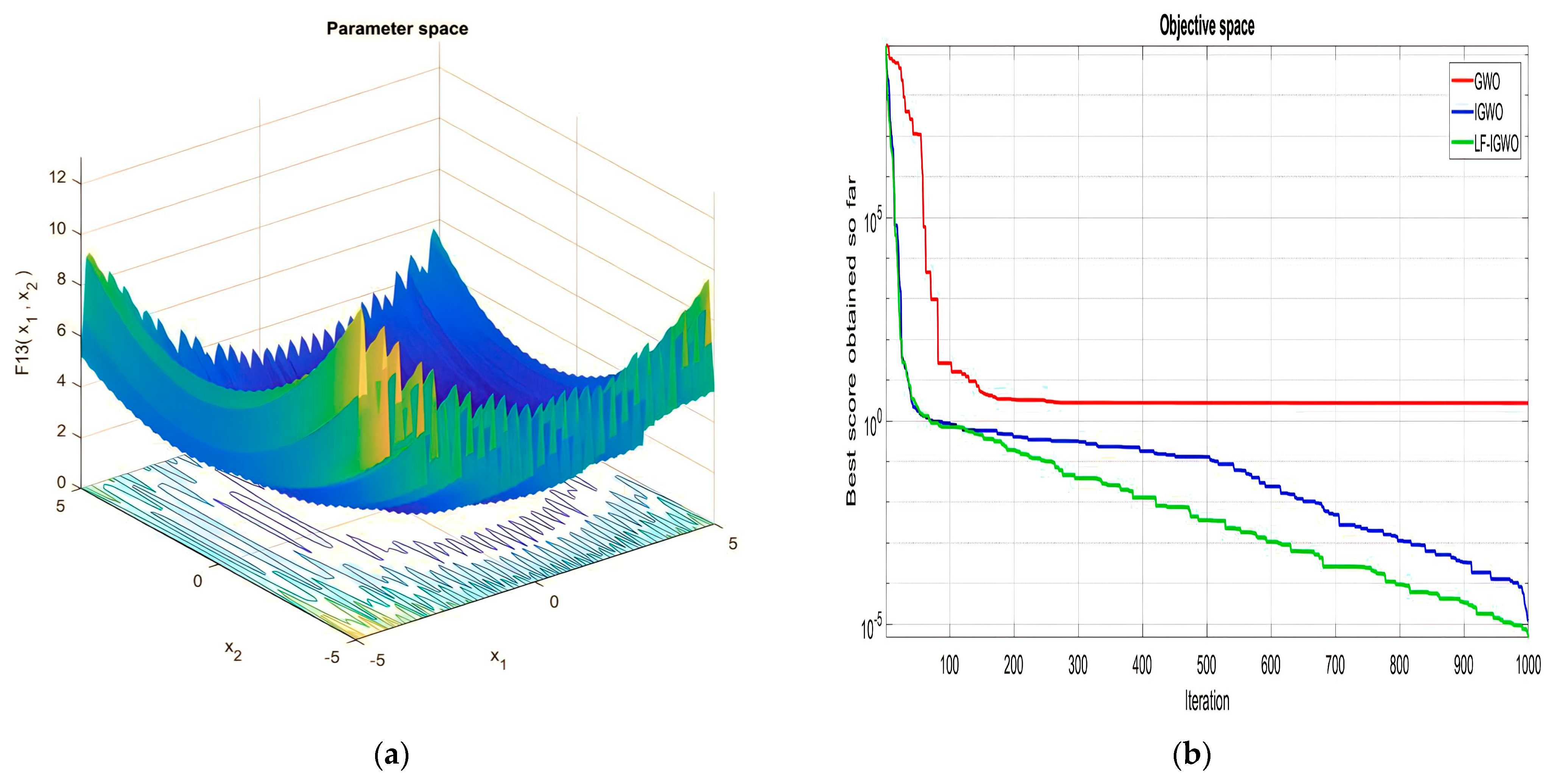
| F13 | 2.53 × 10⁻³ | 1.29 × 10⁻¹ | 12.67 × 10 | 9.72 × 10⁻² | 2.24 × 10⁻¹⁰ | 8.98 × 10⁻⁶ |
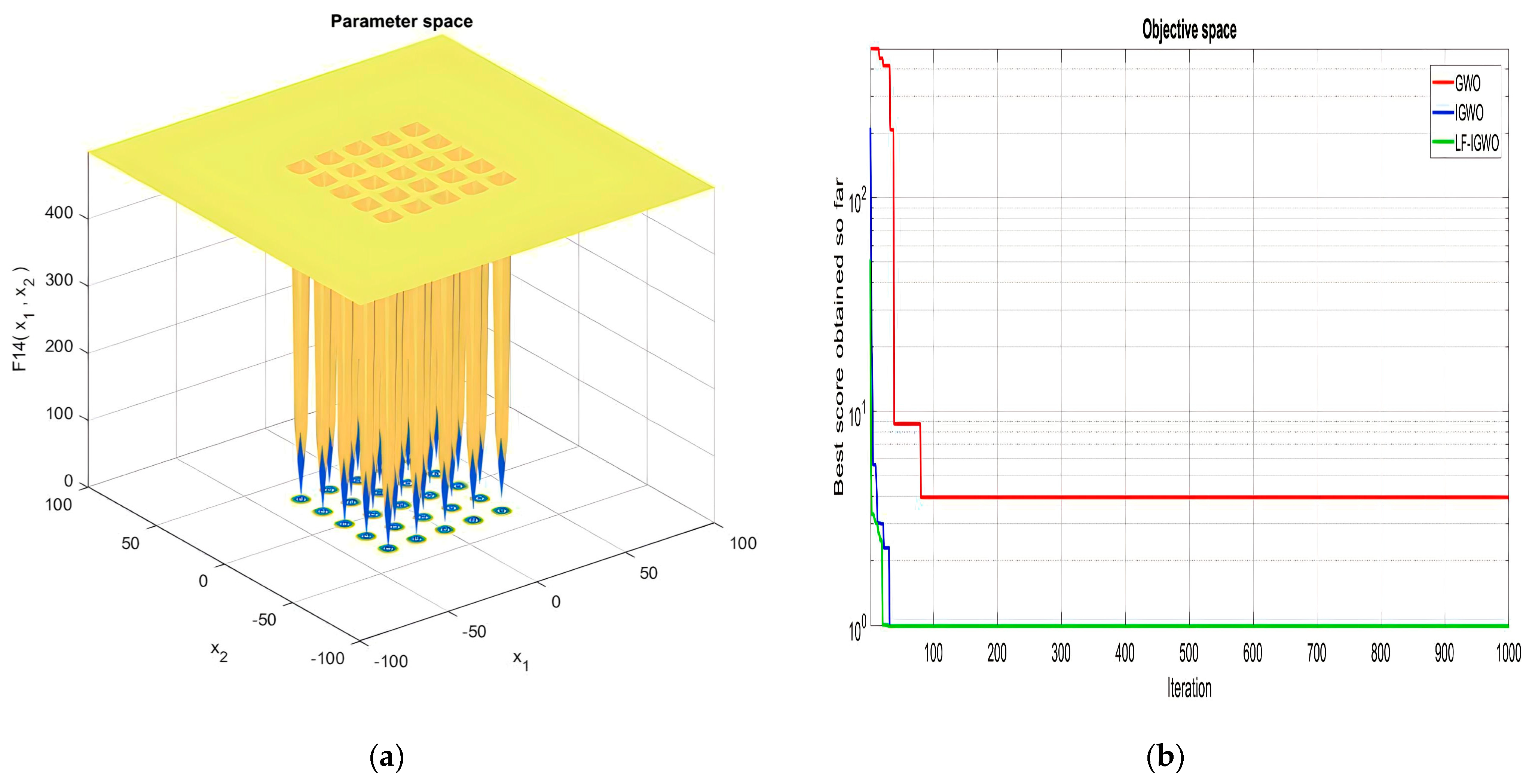
| F14 | 3.46 × 100 | 1.26 × 100 | 7.87 × 100 | 9.98 × 10⁻¹ | 1.16 × 100 | 9.98 × 10⁻¹ |
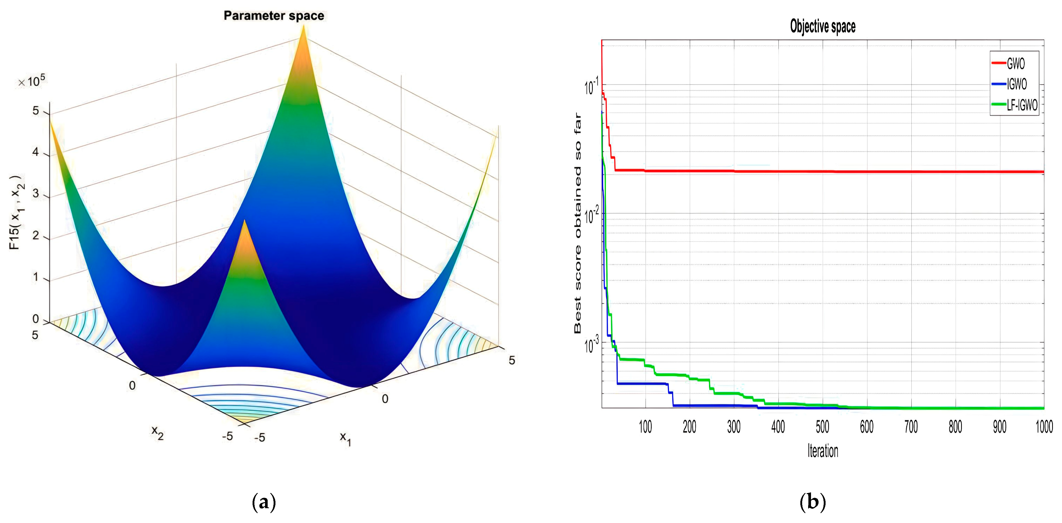
| F15 | 8.94 × 10⁻⁴ | 4.00 × 10⁻³ | 4.54 × 10⁻⁴ | 3.07 × 10⁻⁴ | 1.48 × 10⁻⁴ | 3.07 × 10⁻⁴ |
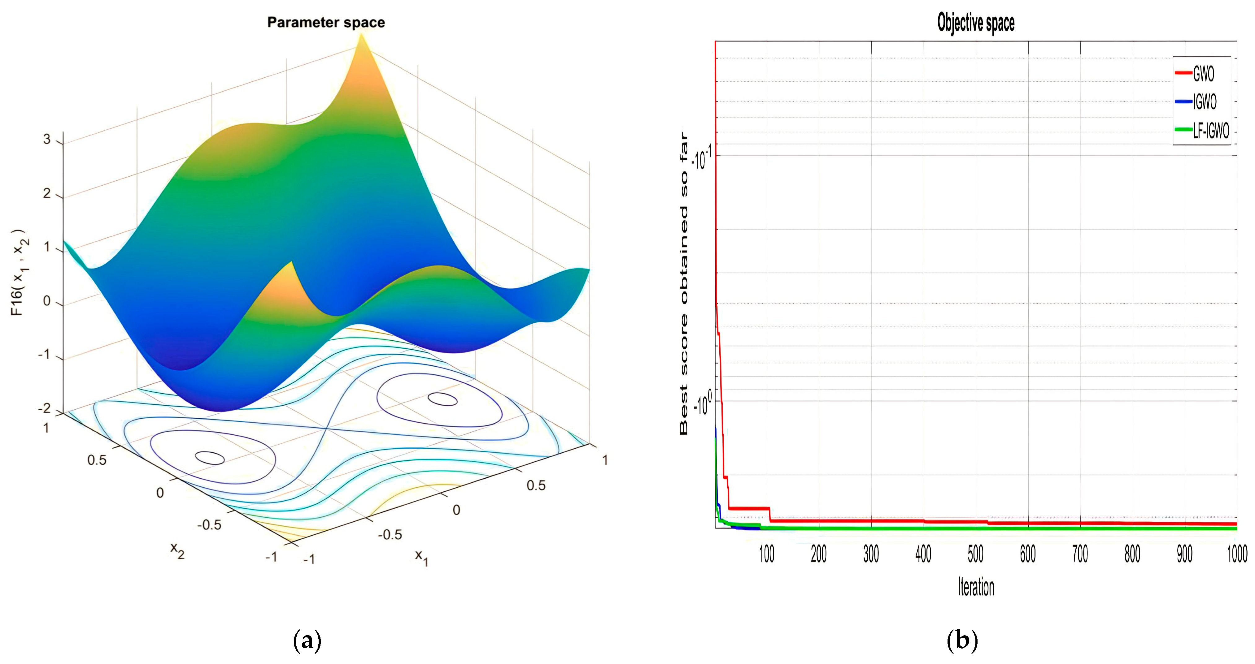
| F16 | −1.03 × 100 | −1.03 × 100 | −1.03 × 100 | −1.03 × 100 | −1.03 × 100 | −1.03 × 100 |
| F17 | 3.99 × 10⁻¹ | 4.00 × 10⁻¹ | 3.98 × 10⁻¹ | 3.97 × 10⁻¹ | 3.98 × 10⁻¹ | 3.097 × 10⁻¹ |
| F18 | 3.00 × 100 | 5.70 × 100 | 3.00 × 100 | 3.00 × 100 | 3.00 × 100 | 3.00 × 100 |
| F19 | −3.86 × 100 | −3.86 × 100 | −3.86 × 100 | −3.86 × 100 | −3.86 × 100 | −3.86 × 100 |
| F20 | −3.27 × 100 | −3.31 × 100 | −3.24 × 100 | −3.32 × 100 | −3.32 × 100 | −3.32 × 100 |
| F21 | −8.60 × 100 | −5.66 × 100 | −5.05 × 100 | −10.15 × 100 | −8.60 × 100 | −10.15 × 100 |
| F22 | −9.07 × 100 | −7.34 × 100 | −10.39 × 100 | −10.40 × 100 | −1.04 × 101 | −10.40 × 100 |
| F23 | −9.20 × 100 | −6.25 × 100 | −1.04 × 101 | −1.05 × 101 | −1.05 × 101 | −1.05 × 101 |
| Function Number | PSO | SSR | GWO | I-GWO | LF-IGWO |
|---|---|---|---|---|---|
| F1 | 1.50 × 10¹¹ | 1.11 × 10¹¹ | 3.00 × 10¹⁰ | 1.59 × 10¹⁰ | 5.04 × 10⁷ |
| F2 | 2.64 × 10⁸ | 1.00 × 10⁹ | 2.84 × 10⁷ | 3.49 × 10⁶ | 4.68 × 10⁵ |
| F3 | 4.12 × 10⁶ | 1.51 × 10⁸ | 5.19 × 10⁴ | 8.59 × 10⁴ | 2.92 × 10⁴ |
| F4 | 4.53 × 10⁴ | 2.38 × 10⁴ | 5.30 × 10³ | 1.082 × 10³ | 491.677 |
| F5 | 1.13 × 10³ | 1.00 × 10³ | 778.48 | 787.30 | 564.402 |
| F6 | 751.76 | 699.66 | 660.77 | 646.87 | 601.758 |
| F7 | 3.37 × 10³ | 1.76 × 10³ | 1.22 × 10³ | 1.45 × 10³ | 805.982 |
| F8 | 1.37 × 10³ | 1.28 × 10³ | 1.05 × 10³ | 1.068 × 10³ | 849.817 |
| F9 | 4.47 × 10⁴ | 2.51 × 10⁴ | 5.48 × 10³ | 6.911 × 10³ | 1.07 × 10³ |
| F10 | 1.19 × 10⁴ | 1.08 × 10⁴ | 6.32 × 10³ | 7.529 × 10³ | 3.01 × 10³ |
| F11 | 5.02 × 10⁴ | 1.18 × 10⁴ | 4.44 × 10³ | 2.379 × 10³ | 1.31 × 10³ |
| F12 | 3.44 × 10¹⁰ | 1.66 × 10¹⁰ | 7.21 × 10⁹ | 3.58 × 10⁸ | 4.38 × 10⁶ |
| F13 | 3.82 × 10¹⁰ | 2.06 × 10¹⁰ | 2.89 × 10⁹ | 6.27 × 10⁷ | 2.68 × 10⁴ |
| F14 | 1.59 × 10⁸ | 2.59 × 10⁷ | 1.71 × 10⁴ | 5.87 × 10⁴ | 3.92 × 10³ |
| F15 | 8.30 × 10⁹ | 4.22 × 10⁹ | 1.94 × 10⁴ | 1.03 × 10⁷ | 1.11 × 10⁴ |
| F16 | 9.62 × 10³ | 1.30 × 10⁴ | 3.566 × 10³ | 3.184 × 10³ | 2.10 × 10³ |
| F17 | 1.56 × 10⁵ | 7.15 × 10³ | 2.269 × 10³ | 2.458 × 10³ | 1.78 × 10³ |
| F18 | 9.70 × 10⁸ | 2.56 × 10⁸ | 7.17 × 10⁵ | 1.05 × 10⁵ | 5.98 × 10⁴ |
| F19 | 7.79 × 10⁹ | 1.00 × 10⁹ | 1.77 × 10⁶ | 2.70 × 10⁷ | 2.13 × 10⁴ |
| F20 | 4.09 × 10³ | 4.11 × 10³ | 2.240 × 10³ | 2.484 × 10³ | 2.20 × 10³ |
| F21 | 2.98 × 10³ | 2.79 × 10³ | 2.577 × 10³ | 2.552 × 10³ | 2.36 × 10³ |
| F22 | 1.22 × 10⁴ | 1.29 × 10⁴ | 6.644 × 10³ | 4.186 × 10³ | 2.44 × 10³ |
| F23 | 4.27 × 10³ | 4.01 × 10³ | 3.207 × 10³ | 2.902 × 10³ | 2.70 × 10³ |
| F24 | 4.49 × 10³ | 4.41 × 10³ | 3.377 × 10³ | 3.071 × 10³ | 2.87 × 10³ |
| F25 | 2.35 × 10⁴ | 6.47 × 10³ | 4.228 × 10³ | 3.669 × 10³ | 2.94 × 10³ |
| F26 | 2.02 × 10⁴ | 1.32 × 10⁴ | 9.251 × 10³ | 5.105 × 10³ | 3.40 × 10³ |
| F27 | 4.90 × 10³ | 5.86 × 10³ | 3.798 × 10³ | 3.298 × 10³ | 3.20 × 10³ |
| F28 | 1.56 × 10⁴ | 1.04 × 10⁴ | 5.270 × 10³ | 3.686 × 10³ | 3.33 × 10³ |
| F29 | 6.16 × 10⁴ | 5.22 × 10⁴ | 5.208 × 10³ | 4.106 × 10³ | 3.56 × 10³ |
| F30 | 8.49 × 10⁹ | 3.25 × 10⁹ | 2.1 × 10⁸ | 1.86 × 10⁷ | 4.53 × 10⁵ |
| Angles | LF-IGWO | IGWO | GWO | PSO |
|---|---|---|---|---|
| A1 | 0.036788 | −0.25222 | 0.2074 | 0.2675 |
| A2 | 0.84503 | 0.73168 | 0 | −0.6905 |
| A3 | 0.24646 | 0.13577 | 0.6342 | −0.3538 |
| A4 | 0.94454 | −0.87421 | 0.0864 | 0.8315 |
| A5 | 0.17788 | 0.18032 | 0.5053 | −0.3885 |
| A6 | 0.69653 | −0.26365 | 0.0428 | 1.1988 |
| A7 | 0.47166 | 0.33732 | 0.0575 | −0.7247 |
| A8 | 0.29501 | 0.42087 | 0.1335 | −1.0523 |
| A9 | 0.4211 | −0.4421 | 0.74 | 0.8072 |
| A10 | 0.77193 | 0.5118 | 0.3837 | 0.9868 |
| A11 | 1.2306 | −0.086737 | 0.3183 | 0.2315 |
| A12 | 0.56625 | −0.48201 | 0.5527 | −0.4606 |
| A13 | 0.11742 | −0.010185 | 0.8574 | 0.0215 |
| A14 | 0.63186 | 0.071222 | 0.2855 | −0.1755 |
| A15 | 0.36631 | 0.67509 | 0.4286 | −0.3821 |
| Algorithm | LF-IGWO | IGWO | GWO | PSO |
|---|---|---|---|---|
| THD (%) | 4.54 | 13.81 | 14.68 | 5.92 |
| Algorithms | d | D2 | N | Op. Value |
|---|---|---|---|---|
| LF-IGWO | 0.0527485 | 0.367865 | 10.665 | 0.01267 |
| IGWO | 0.0517029 | 0.356964 | 11.2893 | 0.012681 |
| GWO | 0.05169 | 0.3567 | 11.2888 | 0.012666 |
| PSO | 0.051728 | 0.357644 | 11.24454 | 0.012674 |
| GA | 0.05148 | 0.35166 | 11.6322 | 0.012704 |
| Algorithms | Op. Value | ||||
|---|---|---|---|---|---|
| LF-IGWO | 0.8021493 | 0.5113717 | 41.54997 | 183.573 | 6282.2292 |
| GWO | 0.8125 | 0.4345 | 42.089181 | 176.758731 | 6051.5639 |
| GA | 0.8125 | 0.4345 | 40.3239 | 200 | 6288.7445 |
| PSO | 0.883044 | 0.533053 | 45.38829 | 190.0616 | 7865.233 |
| IGWO | 0.9035907 | 0.5319827 | 44.20703 | 154.0763 | 6793.5848 |
| Function Number | PSO | GA | GWO | IGWO | SSR |
|---|---|---|---|---|---|
| F1 | 0.001588 | 0.000156 | 0.003177 | 0.027086 | 0.10499 |
| F2 | 0.004522 | 0.000145 | 0.003177 | 0.18577 | 0.10499 |
| F3 | 0.000145 | 0.000145 | 0.000145 | 1 | 0.10499 |
| F4 | 0.009524 | 0.000145 | 0.000145 | 0.37904 | 0.10499 |
| F5 | 0.000145 | 0.28378 | 0.000145 | 0.077272 | 0.10499 |
| F6 | 0.000145 | 0.000145 | 0.000145 | 0.27071 | 0.10499 |
| F7 | 0.0001268 | 0.10499 | 0.000145 | 0.48252 | 0.10499 |
| F8 | 0.30815 | 0.37904 | 0.31815 | 0.28378 | 0.10499 |
| F9 | 0.62527 | 0.69913 | 0.10221 | 0.98231 | 0.10499 |
| F10 | 0.000294 | 0.000156 | 0.000145 | 0.23985 | 0.10499 |
| F11 | 0.000156 | 0.000156 | 0.000145 | 0.46427 | 0.10499 |
| F12 | 0.351889 | 0.000145 | 0.000145 | 0.063533 | 0.10499 |
| F13 | 0.168452 | 0.000156 | 0.000145 | 0.59969 | 0.10499 |
| F14 | 0.061837 | 0.01857 | 0.071429 | 0.66667 | 0.66667 |
| F15 | 0.62483 | 0.35684 | 0.47619 | 0.88571 | 0.4 |
| F16 | 0.07467 | 0.071429 | 0.071429 | 0.66667 | 0.66667 |
| F17 | 0.071498 | 0.071429 | 0.071429 | 0.66667 | 0.66667 |
| F18 | 0.072795 | 0.66667 | 0.071429 | 1 | 0.66667 |
| F19 | 0.069426 | 0.061584 | 0.071429 | 0.7 | 0.5 |
| F20 | 0.49509 | 0.51455 | 0.48485 | 0.69913 | 0.28571 |
| F21 | 0.0064732 | 0.0008616 | 0.009524 | 0.68571 | 0.4 |
| F22 | 0.018654 | 0.02666 | 0.009524 | 0.88571 | 0.4 |
| F23 | 0.72364 | 0.5426 | 0.009524 | 1 | 0.4 |
| Tension Compression Spring | 0.7569 | 0.6 | 0.71429 | 1 | 0.5 |
| Welded Beam | 0.09852 | 0.854554 | 0.47619 | 0.68571 | 1 |
| Pressure Vessel | 0.09852 | 0.854554 | 0.25714 | 0.68571 | 1 |
Disclaimer/Publisher’s Note: The statements, opinions and data contained in all publications are solely those of the individual author(s) and contributor(s) and not of MDPI and/or the editor(s). MDPI and/or the editor(s) disclaim responsibility for any injury to people or property resulting from any ideas, methods, instructions or products referred to in the content. |
© 2023 by the authors. Licensee MDPI, Basel, Switzerland. This article is an open access article distributed under the terms and conditions of the Creative Commons Attribution (CC BY) license (https://creativecommons.org/licenses/by/4.0/).
Share and Cite
Bhatt, B.; Sharma, H.; Arora, K.; Joshi, G.P.; Shrestha, B. Levy Flight-Based Improved Grey Wolf Optimization: A Solution for Various Engineering Problems. Mathematics 2023, 11, 1745. https://doi.org/10.3390/math11071745
Bhatt B, Sharma H, Arora K, Joshi GP, Shrestha B. Levy Flight-Based Improved Grey Wolf Optimization: A Solution for Various Engineering Problems. Mathematics. 2023; 11(7):1745. https://doi.org/10.3390/math11071745
Chicago/Turabian StyleBhatt, Bhargav, Himanshu Sharma, Krishan Arora, Gyanendra Prasad Joshi, and Bhanu Shrestha. 2023. "Levy Flight-Based Improved Grey Wolf Optimization: A Solution for Various Engineering Problems" Mathematics 11, no. 7: 1745. https://doi.org/10.3390/math11071745
APA StyleBhatt, B., Sharma, H., Arora, K., Joshi, G. P., & Shrestha, B. (2023). Levy Flight-Based Improved Grey Wolf Optimization: A Solution for Various Engineering Problems. Mathematics, 11(7), 1745. https://doi.org/10.3390/math11071745