Kinetics of a Reaction-Diffusion Mtb/SARS-CoV-2 Coinfection Model with Immunity

Abstract

The severe acute respiratory syndrome coronavirus 2 (SARS-CoV-2) and Mycobacterium tuberculosis (Mtb) coinfection has been observed in a number of nations and it is connected with severe illness and death. The paper studies a reaction–diffusion within-host Mtb/SARS-CoV-2 coinfection model with immunity. This model explores the connections between uninfected epithelial cells, latently Mtb-infected epithelial cells, productively Mtb-infected epithelial cells, SARS-CoV-2-infected epithelial cells, free Mtb particles, free SARS-CoV-2 virions, and CTLs. The basic properties of the model’s solutions are verified. All equilibrium points with the essential conditions for their existence are calculated. The global stability of these equilibria is established by adopting compatible Lyapunov functionals. The theoretical outcomes are enhanced by implementing numerical simulations. It is found that the equilibrium points mirror the single infection and coinfection states of SARS-CoV-2 with Mtb. The threshold conditions that determine the movement from the monoinfection to the coinfection state need to be tested when developing new treatments for coinfected patients. The impact of the diffusion coefficients should be monitored at the beginning of coinfection as it affects the initial distribution of particles in space.

1. Introduction

Coronavirus disease 2019 (COVID-19) is a viral disease induced by severe acute respiratory syndrome coronavirus 2 (SARS-CoV-2) and emerged in 2019. Although the number of new cases decreased in the last few months, COVID-19 is continuing its spread around the globe [1]. Following the World Health Organization (WHO) report issued on 1 March 2023, above 758,000,000 affirmed cases and over 6,800,000 deaths have been accounted globally [1]. COVID-19 coinfections with other viral or bacterial diseases are common, which complicates the treatment of COVID-19 [2]. Tuberculosis (TB) is a bacterial infection attributable to Mycobacterium tuberculosis (Mtb). Currently, COVID-19 co-occurring with TB has been declared in a number of nations [3]. As COVID-19 and TB are greatly infectious diseases, understanding Mtb/SARS-CoV-2 coinfection is very crucial for protection and treatment of coinfection.

SARS-CoV-2 is an enveloped RNA virus which is linked with the Betacoronavirus genus [4]. It breaks into the host cell using the angiotensin-converting enzyme 2 (ACE2) receptor [5]. It primarily infects the alveolar epithelial type-II cells of the lungs [6]. Similar to SARS-CoV-2, Mtb infects alveolar epithelial type-II cells through pattern recognition receptors such as toll-like receptors, complement receptors, and CD14 receptors [7]. Thus, the lung is the major infection site for these pathogens. Nevertheless, they can invade cells within different organs [6]. Since SARS-CoV-2 and Mtb infect the same target, this could increase the seriousness of disease in coinfected people [4]. Both pathogens are disseminated through respiratory droplets [2]. The most dominant features of Mtb/SARS-CoV-2 co-occurring are fever, cough, and dyspenea [2]. Risk factors in coinfection include age and comorbidities such as diabetes, HIV, and hypertension [2,3]. The immune response in coinfection includes T cells [8]. Specifically, cytotoxic T lymphocytes (CTLs) work on eliminating infected cells from the body. In the mild cases, the immune response can clear both infections. It has been proposed that Mtb/SARS-CoV-2 patients are at higher risk of death and developing severe disease than SARS-CoV-2 patients without Mtb [2,3,8]. Moreover, some studies reported that SARS-CoV-2 infection may cause latent Mtb to become active in coinfected people [3,4]. Other studies also observed that coinfected patients have low lymphocyte counts [2,8]. Thus, understanding the mechanism of coinfection is very important to evolve treatments for coinfected patients.

Mathematical models have been utilized to assist experimental and medical studies of different infections. These models are partitioned into epidemiological and within-host models. Epidemiological systems consider the interactions between individuals at the population level, while within-host systems explore the interplay between pathogens and cells within the host’s body. A variety of COVID-19 epidemiological models (see for example, [9,10,11,12,13,14,15]) and within-host models (see for example, [16,17,18]) have been introduced and investigated. Similarly, TB models have been widely studied as epidemiological models (see for example, [19,20,21,22]) and within-host models (see for example, [23,24,25,26,27]). Some coinfection models of COVID-19 with other diseases have been developed. For instance, Pinky and Dobrovolny [28] analyzed a model that tests the impact of SARS-CoV-2 coinfection with the influenza virus. Al Agha and Elaiw [29] established a within-host SARS-CoV-2/malaria model with immune response. Elaiw et al. [30] developed a SARS-CoV-2/HIV coinfection model that takes the latent stage of infected epithelial cells (EPCs) into consideration. Elaiw and Al Agha [31] studied a SARS-CoV-2/cancer system with two immune responses.

Many epidemiological models of TB/COVID-19 coinfection have been proposed (see for example, [32,33,34]). On the other hand, within-host models are not widely considered. In [35], a within-host coinfection model has been formalized using ordinary differential Equations (ODEs). This work develops a reaction–diffusion within-host Mtb/SARS-CoV-2 coinfection model. It depicts the interplay between uninfected EPCs, latently Mtb-infected EPCs, productively Mtb-infected EPCs, SARS-CoV-2-infected EPCs, Mtb particles, SARS-CoV-2 particles, and CTLs. Additionally, this model is formalized using partial differential Equations (PDEs) which count the nonuniform distribution of cells and pathogens with their ability to move. Thus, PDEs are more realistic than ODEs which assume the spatial distribution homogeneity of cells and particles. Using the developed model, we (i) establish the boundedness and nonnegativity of the solutions, (ii) determine all equilibrium points and find the thresholds, (iii) confirm the global stability of each point, and (iv) use numerical simulations to validate the theoretical observations.

The remaining sections are divided as follows. Section 2 represents the model. Section 3 proves the boundedness and nonnegativity of the solutions. Moreover, it recounts all equilibrium points. Section 4 employs Lyapunov functionals to show the global stability of each point. Section 5 implements numerical simulations. The last section provides the conclusion with upcoming works.

2. A Reaction–Diffusion Mtb/SARS-CoV-2 Coinfection Model

This part describes the model under consideration. In this model, we assume that Mtb and SARS-CoV-2 have the same target, and CTLs kill infected cells at the same rate. The model consists of seven PDEs as follows:

$$\{\begin{array}{l}\frac{\partial U(x,t)}{\partial t}=D_U\Delta U+\lambda -{\eta }_{1}UB-{\eta }_{2}UV-{ϵ}_{1}U,\\ \frac{\partial L(x,t)}{\partial t}=D_L\Delta L+{\eta }_{1}UB-aL,\\ \frac{\partial I^B(x,t)}{\partial t}=D_{I^B}\Delta I^B+aL-\gamma I^{B}Z-{ϵ}_2{I}^B,\\ \frac{\partial I^V(x,t)}{\partial t}=D_{I^V}\Delta I^V+{\eta }_{2}UV-\gamma I^{V}Z-{ϵ}_3{I}^V,\\ \frac{\partial B(x,t)}{\partial t}=D_B\Delta B+{\mu }_1{ϵ}_2{I}^B-{ϵ}_{4}B,\\ \frac{\partial V(x,t)}{\partial t}=D_V\Delta V+{\mu }_2{I}^V-{ϵ}_{5}V,\\ \frac{\partial Z(x,t)}{\partial t}=D_Z\Delta Z+\omega I^{B}Z+\omega I^{V}Z-{ϵ}_{6}Z,\end{array}$$

(1)

where the time $t>0$ and the position $x\in \Psi$. The domain $\Psi$ is bounded and connected with a smooth boundary $\partial \Psi$. The compartments U, L, $I^B$, $I^V$, B, V, and Z designate the concentrations of uninfected EPCs, latently Mtb-infected EPCs, productively Mtb-infected EPCs, SARS-CoV-2-infected EPCs, Mtb particles, SARS-CoV-2 particles, and CTLs at $(x,t)$, respectively. Uninfected EPCs are generated at rate $\lambda$. Mtb converts healthy EPCs into latently infected cells at rate ${\eta }_{1}UB$, while SARS-CoV-2 infects the same type of cells at rate ${\eta }_{2}UV$. Latently Mtb-infected cells become an active producer at rate $aL$. Mtb particles are created at a total production rate ${\mu }_1{ϵ}_2{I}^B$. SARS-CoV-2 virions are ejected from SARS-CoV-2-infected cells at rate ${\mu }_2{I}^V$. CTLs remove Mtb and SARS-CoV-2 infected cells at rates $\gamma I^{B}Z$ and $\gamma I^{V}Z$, respectively. The corresponding stimulation rates are $\omega I^{B}Z$ and $\omega I^{V}Z$, respectively. The compartments U, $I^B$, $I^V$, B, V, and Z die at rates ${ϵ}_{1}U$, ${ϵ}_2{I}^B$, ${ϵ}_3{I}^V$, ${ϵ}_{4}B$, ${ϵ}_{5}V$, and ${ϵ}_{6}Z$, respectively. We assume that each compartment K diffuses with a diffusion coefficient $D_K$. The operator $\Delta =\frac{{\partial }^2}{\partial x^2}$ is the Laplacian operator. We presume that all parameters of model (1) are positive. The initial conditions (ICs) of system (1) are

$$\begin{array}{cc}& U(x,0)={\nu }_1\left(x\right),L(x,0)={\nu }_2\left(x\right),I^B(x,0)={\nu }_3\left(x\right),I^V(x,0)={\nu }_4\left(x\right),\hfill \\ & B(x,0)={\nu }_5\left(x\right),V(x,0)={\nu }_6\left(x\right),Z(x,0)={\nu }_7\left(x\right),x\in \overline{\Psi },\hfill \end{array}$$

(2)

where ${\nu }_i\left(x\right)\ge 0$, $i=1,2,\dots ,7$, are continuous functions in $\overline{\Psi }$. The boundary conditions (BCs) of (1) are

$$\frac{\partial U}{\partial \overrightarrow{r}}=\frac{\partial L}{\partial \overrightarrow{r}}=\frac{\partial I^B}{\partial \overrightarrow{r}}=\frac{\partial I^V}{\partial \overrightarrow{r}}=\frac{\partial B}{\partial \overrightarrow{r}}=\frac{\partial V}{\partial \overrightarrow{r}}=\frac{\partial Z}{\partial \overrightarrow{r}}=0,t>0,x\in \partial \Psi ,$$

(3)

where ${\displaystyle \frac{\partial }{\partial \overrightarrow{r}}}$ is the outward normal derivative on $\partial \Psi$. These Neumann BCs suggest that the boundary is isolated.

In the upcoming parts of the paper and for simplicity, we consider the contraction $K(x,t)\equiv K$ for each compartment K in model (1).

3. Basic Properties

This section certifies that the solutions of system (1)–(3) are unique, nonnegative, and bounded. Additionally, it computes all equilibrium points of model (1).

Let $\mathbb{S}=BUC\left(\overline{\Psi },{\mathbb{R}}^7\right)$ be the set of functions that are bounded and continuous from $\overline{\Psi }$ to ${\mathbb{R}}^7$. The positive cone ${\mathbb{S}}_{+}=BUC\left(\overline{\Psi },{\mathbb{R}}_{+}^7\right)\subset \mathbb{S}$ forms a partial order on $\mathbb{S}$. Define ${\parallel f\parallel }_{\mathbb{S}}=\underset{x\in \overline{\Psi }}{sup}\left|f\left(x\right)\right|$. Consequently, $\left({\mathbb{S},\parallel ·\parallel }_{\mathbb{S}}\right)$ is a Banach lattice [36,37].

Theorem 1.

Suppose that $D_U=D_L=D_{I^B}=D_{I^V}=D_Z=D_1$. Then, model (1) with any ICs (2) has a unique, nonnegative, and bounded solution on $\overline{\Psi }\times [0,+\infty )$.

Proof. 

For any $\nu ={({\nu }_1,{\nu }_2,{\nu }_3,{\nu }_4,{\nu }_5,{\nu }_6,{\nu }_7)}^T\in {\mathbb{S}}_{+}$, we define $P={(P_1,P_2,P_3,P_4,P_5,P_6,P_7)}^T:{\mathbb{S}}_{+}\to \mathbb{S}$ by

$$\{\begin{array}{l}{P}_1\left(\nu \right)\left(x\right)=\lambda -{\eta }_1{\nu }_1\left(x\right){\nu }_5\left(x\right)-{\eta }_2{\nu }_1\left(x\right){\nu }_6\left(x\right)-{ϵ}_1{\nu }_1\left(x\right),\\ P_2\left(\nu \right)\left(x\right)={\eta }_1{\nu }_1\left(x\right){\nu }_5\left(x\right)-a{\nu }_2\left(x\right),\\ P_3\left(\nu \right)\left(x\right)=a{\nu }_2\left(x\right)-\gamma {\nu }_3\left(x\right){\nu }_7\left(x\right)-{ϵ}_2{\nu }_3\left(x\right),\\ P_4\left(\nu \right)\left(x\right)={\eta }_2{\nu }_1\left(x\right){\nu }_6\left(x\right)-\gamma {\nu }_4\left(x\right){\nu }_7\left(x\right)-{ϵ}_3{\nu }_4\left(x\right),\\ P_5\left(\nu \right)\left(x\right)={\mu }_1{ϵ}_2{\nu }_3\left(x\right)-{ϵ}_4{\nu }_5\left(x\right),\\ P_6\left(\nu \right)\left(x\right)={\mu }_2{\nu }_4\left(x\right)-{ϵ}_5{\nu }_6\left(x\right),\\ P_7\left(\nu \right)\left(x\right)=\omega {\nu }_3\left(x\right){\nu }_7\left(x\right)+\omega {\nu }_4\left(x\right){\nu }_7\left(x\right)-{ϵ}_6{\nu }_7\left(x\right).\end{array}$$

We observe that P is Lipschitz on ${\mathbb{S}}_{+}$. Therefore, it is possible to rewrite system (1)–(3) as the abstract DE:

$$\{\begin{array}{l}\frac{dJ}{dt}=DJ+P\left(J\right),t>0,\\ J_0=\nu \in {\mathbb{S}}_{+},\end{array}$$

where $J={(U,L,I^B,I^V,B,V,Z)}^T$ and $DJ=(D_U\Delta U,D_L\Delta L,D_{I^B}\Delta I^B,D_{I^V}\Delta I^V,D_B\Delta B$, $D_V\Delta V,D_Z{\Delta Z)}^T$. We can show that

$$\underset{h\to 0^{+}}{lim}\frac{1}{h}\mathrm{dist}\left(\nu +hP\left(\nu \right),{\mathbb{S}}_{+}\right)=0,\nu \in {\mathbb{S}}_{+}.$$

Hence, for any $\nu \in {\mathbb{S}}_{+}$, model (1)–(3) has a unique nonnegative mild solution for the time interval $[0,T_e)$.

To verify the boundedness, we consider the function

$${\mathrm{Y}}_1(x,t)=U+L+I^V.$$

$As$$D_U=D_L=D_{I^V}=D_1$, then by utilizing model (1) we obtain

$$\begin{array}{cc}\frac{\partial {\mathrm{Y}}_1}{\partial t}-D_1\Delta {\mathrm{Y}}_1& =\lambda -{ϵ}_{1}U-aL-\gamma I^{V}Z-{ϵ}_3{I}^V\hfill \\ & \le \lambda -{ϵ}_{1}U-aL-{ϵ}_3{I}^V\hfill \\ & \le \lambda -{\sigma }_1\left[U+L+I^V\right]\hfill \\ & =\lambda -{\sigma }_1{\mathrm{Y}}_1,\hfill \end{array}$$

where ${\sigma }_1=min\left\{a,{ϵ}_1,{ϵ}_3\right\}$. Thus, ${\mathrm{Y}}_1$ satisfies the system

$$\{\begin{array}{l}\frac{\partial {\mathrm{Y}}_1}{\partial t}-D_1\Delta {\mathrm{Y}}_1\le \lambda -{\sigma }_1{\mathrm{Y}}_1,\\ \frac{\partial {\mathrm{Y}}_1}{\partial \overrightarrow{r}}=0,\\ {\mathrm{Y}}_1(x,0)\ge 0.\end{array}$$

Assume that ${\tilde{\mathrm{Y}}}_1\left(t\right)$ satisfies the system

$$\{\begin{array}{l}\frac{d{\tilde{\mathrm{Y}}}_1\left(t\right)}{dt}=\lambda -{\sigma }_1{\tilde{\mathrm{Y}}}_1\left(t\right),\\ {\tilde{\mathrm{Y}}}_1\left(0\right)={\displaystyle \underset{x\in \overline{\Psi }}{max}}{\mathrm{Y}}_1(x,0),\end{array}$$

which implies that ${\tilde{\mathrm{Y}}}_1\left(t\right)\le max\left\{{\displaystyle \frac{\lambda }{{\sigma }_1}},{\displaystyle \underset{x\in \overline{\Psi }}{max}}{\mathrm{Y}}_1(x,0)\right\}$. In accord with the comparison principle (CP) [38], we obtain ${\mathrm{Y}}_1(x,t)\le {\tilde{\mathrm{Y}}}_1\left(t\right)$. As a result, we have

$${\mathrm{Y}}_1(x,t)\le max\left\{{\displaystyle \frac{\lambda }{{\sigma }_1}},{\displaystyle \underset{x\in \overline{\Psi }}{max}}{\mathrm{Y}}_1(x,0)\right\}:=Q_1.$$

This ensures that U, L, and $I^V$ are bounded. From the third equation of (1), we have

$$\begin{array}{cc}\frac{\partial I^B}{\partial t}-D_{I^B}\Delta I^B& =aL-\gamma I^{B}Z-{ϵ}_2{I}^B\hfill \\ & \le aL-{ϵ}_2{I}^B\hfill \\ & \le a{Q}_1-{ϵ}_2{I}^B.\hfill \end{array}$$

We can conclude from the CP [38] that

$$I^B\le max\left\{{\displaystyle \frac{a{Q}_1}{{ϵ}_2}},{\displaystyle \underset{x\in \overline{\Psi }}{max}}{I}^B(x,0)\right\}:=Q_2.$$

Thus, $I^B$ is bounded. From the fifth equation of (1), we have

$$\begin{array}{cc}\frac{\partial B}{\partial t}-D_B\Delta B& ={\mu }_1{ϵ}_2{I}^B-{ϵ}_{4}B\hfill \\ & \le {\mu }_1{ϵ}_2{Q}_2-{ϵ}_{4}B.\hfill \end{array}$$

Based on the CP [38], we obtain

$$B\le max\left\{{\displaystyle \frac{{\mu }_1{ϵ}_2{Q}_2}{{ϵ}_4}},{\displaystyle \underset{x\in \overline{\Psi }}{max}}B(x,0)\right\}.$$

Hence, B is bounded. From the sixth equation of model (1), we obtain

$$\begin{array}{cc}\frac{\partial V}{\partial t}-D_V\Delta V& ={\mu }_2{I}^V-{ϵ}_{5}V\hfill \\ & \le {\mu }_2{Q}_1-{ϵ}_{5}V.\hfill \end{array}$$

The CP [38] implies that

$$V\le max\left\{{\displaystyle \frac{{\mu }_2{Q}_1}{{ϵ}_5}},{\displaystyle \underset{x\in \overline{\Psi }}{max}}V(x,0)\right\}:=Q_3.$$

Thus, V is bounded. Finally, we introduce the function

$${\mathrm{Y}}_2(x,t)=I^B+I^V+\frac{\gamma }{\omega }Z.$$

Then, we obtain

$$\begin{array}{cc}\hfill \frac{\partial {\mathrm{Y}}_2}{\partial t}-D_1\Delta {\mathrm{Y}}_2& =aL+{\eta }_{2}UV-{ϵ}_2{I}^B-{ϵ}_3{I}^V-\frac{\gamma {ϵ}_6}{\omega }Z\hfill \\ & \le a{Q}_1+{\eta }_2{Q}_1{Q}_3-{\sigma }_2{\mathrm{Y}}_2,\hfill \end{array}$$

where ${\sigma }_2=min\left\{{ϵ}_2,{ϵ}_3,{ϵ}_6\right\}$. By the CP, [38], we obtain

$${\mathrm{Y}}_2(x,t)\le max\left\{{\displaystyle \frac{a{Q}_1+{\eta }_2{Q}_1{Q}_3}{{\sigma }_2}},{\displaystyle \underset{x\in \overline{\Psi }}{max}}{\mathrm{Y}}_2(x,0)\right\}.$$

This implies that Z is bounded. The above results show that all solutions are bounded on $\overline{\Psi }\times [0,T_e)$, and so solutions are bounded on $\overline{\Psi }\times [0,+\infty )$. This conclusion is derived from the standard theory for semi-linear parabolic Equations [39]. □

Proposition 1.

The conditions ${\mathcal{R}}_{0B}$, ${\mathcal{R}}_{0V}$, ${\mathcal{R}}_{1B}$, ${\mathcal{R}}_{1V}$, and σ exist such that system (1) has six equilibrium points:

(i) 

The uninfected equilibrium $E_0$ always exists;

(ii) 

The Mtb immune-free equilibrium $E_1$ is defined when ${\mathcal{R}}_{0B}>1$;

(iii) 

The COVID-19 immune-free equilibrium $E_2$ is defined if ${\mathcal{R}}_{0V}>1$;

(iv) 

The Mtb equilibrium with immunity $E_3$ exists if ${\mathcal{R}}_{1B}>1$;

(v) 

The COVID-19 equilibrium with immunity $E_4$ exists if ${\mathcal{R}}_{1V}>1$;

(vi) 

The Mtb/SARS-CoV-2 coinfection equilibrium $E_5$ exists if ${\displaystyle \frac{\omega \lambda {\eta }_2{\mu }_2{ϵ}_4}{{ϵ}_2{ϵ}_5\left[\omega {ϵ}_1{ϵ}_4+{\eta }_1{\mu }_1{ϵ}_2{ϵ}_6\right]}}+1>{\displaystyle \frac{{ϵ}_3}{{ϵ}_2}}+{\mathcal{R}}_{1B}$, ${\displaystyle \frac{\omega \lambda {\eta }_1{\mu }_1{ϵ}_2{ϵ}_5}{{ϵ}_3{ϵ}_4\left[\omega {ϵ}_1{ϵ}_5+{\eta }_2{\mu }_2{ϵ}_6\right]}}+1>{\displaystyle \frac{{ϵ}_2}{{ϵ}_3}}+{\mathcal{R}}_{1V}$, ${\displaystyle \frac{{\mathcal{R}}_{0V}}{{\mathcal{R}}_{0B}}}>1$, ${ϵ}_2>{ϵ}_3$, and $\sigma >1$.

Proof. 

The equilibrium points of Equation (1) can be drawn by solving the system:

$$\{\begin{array}{l}0=\lambda -{\eta }_{1}UB-{\eta }_{2}UV-{ϵ}_{1}U,\\ 0={\eta }_{1}UB-aL,\\ 0=aL-\gamma I^{B}Z-{ϵ}_2{I}^B,\\ 0={\eta }_{2}UV-\gamma I^{V}Z-{ϵ}_3{I}^V,\\ 0={\mu }_1{ϵ}_2{I}^B-{ϵ}_{4}B,\\ 0={\mu }_2{I}^V-{ϵ}_{5}V,\\ 0=\omega I^{B}Z+\omega I^{V}Z-{ϵ}_{6}Z.\end{array}$$

Then, we obtain the following:

(i)

The uninfected equilibrium $E_0=\left(U_0,0,0,0,0,0,0\right)$, where $U_0={\displaystyle \frac{\lambda }{{ϵ}_1}}>0$. Thus, $E_0$ always exists.

(ii)

The Mtb immune-free equilibrium $E_1=\left(U_1,L_1,I_1^B,0,B_1,0,0\right)$. The components are given as follows:

$$U_1=\frac{{ϵ}_4}{{\eta }_1{\mu }_1},L_1=\frac{{ϵ}_1{ϵ}_4}{a{\eta }_1{\mu }_1}\left({\mathcal{R}}_{0B}-1\right),I_1^B=\frac{{ϵ}_1{ϵ}_4}{{\eta }_1{\mu }_1{ϵ}_2}\left({\mathcal{R}}_{0B}-1\right),B_1=\frac{{ϵ}_1}{{\eta }_1}\left({\mathcal{R}}_{0B}-1\right),$$

where ${\mathcal{R}}_{0B}={\displaystyle \frac{\lambda {\eta }_1{\mu }_1}{{ϵ}_1{ϵ}_4}}$. We note that $U_1$ is positive, whilst $L_1$, $I_1^B$, and $B_1$ are positive when ${\mathcal{R}}_{0B}>1$. Hence, $E_1$ exists if ${\mathcal{R}}_{0B}>1$. The parameter ${\mathcal{R}}_{0B}$ appoints the onset of Mtb infection with inactive CTLs.

(iii)

The COVID-19 immune-free equilibrium $E_2=\left(U_2,0,0,I_2^V,0,V_2,0\right)$. Its coordinates are written as follows:

$$U_2=\frac{{ϵ}_3{ϵ}_5}{{\eta }_2{\mu }_2},I_2^V=\frac{{ϵ}_1{ϵ}_5}{{\eta }_2{\mu }_2}\left({\mathcal{R}}_{0V}-1\right),V_2=\frac{{ϵ}_1}{{\eta }_2}\left({\mathcal{R}}_{0V}-1\right),$$

where ${\mathcal{R}}_{0V}={\displaystyle \frac{\lambda {\eta }_2{\mu }_2}{{ϵ}_1{ϵ}_3{ϵ}_5}}$. Thus, $U_2>0$, whilst $I_2^V>0$ and $V_2>0$ when ${\mathcal{R}}_{0V}>1$. Accordingly, $E_2$ is defined when ${\mathcal{R}}_{0V}>1$. The threshold ${\mathcal{R}}_{0V}$ locates the start of COVID-19 infection, where the CTL immunity is inactive.

(iv)

The Mtb equilibrium with immunity $E_3=\left(U_3,L_3,I_3^B,0,B_3,0,Z_3\right)$, where

$$\begin{array}{cc}& U_3={\displaystyle \frac{\omega \lambda {ϵ}_4}{\omega {ϵ}_1{ϵ}_4+{\eta }_1{\mu }_1{ϵ}_2{ϵ}_6}},L_3=\frac{\lambda {\eta }_1{\mu }_1{ϵ}_2{ϵ}_6}{a\left[\omega {ϵ}_1{ϵ}_4+{\eta }_1{\mu }_1{ϵ}_2{ϵ}_6\right]},I_3^B=\frac{{ϵ}_6}{\omega },\hfill \\ & B_3=\frac{{\mu }_1{ϵ}_2{ϵ}_6}{\omega {ϵ}_4},Z_3=\frac{{ϵ}_2}{\gamma }\left({\mathcal{R}}_{1B}-1\right),\hfill \end{array}$$

where ${\mathcal{R}}_{1B}={\displaystyle \frac{\omega \lambda {\eta }_1{\mu }_1}{\omega {ϵ}_1{ϵ}_4+{\eta }_1{\mu }_1{ϵ}_2{ϵ}_6}}$. We note that $U_3$, $L_3$, $I_3^B$ and $B_3$ are always positive, while $Z_3>0$ if ${\mathcal{R}}_{1B}>1$. This implies that $E_3$ exists if ${\mathcal{R}}_{1B}>1$. The threshold ${\mathcal{R}}_{1B}$ sets the activation of CTLs versus Mtb-infected EPCs.

(v)

The COVID-19 equilibrium with immunity $E_4=\left(U_4,0,0,I_4^V,0,V_4,Z_4\right)$. The components are given as

$$U_4={\displaystyle \frac{\omega \lambda {ϵ}_5}{\omega {ϵ}_1{ϵ}_5+{\eta }_2{\mu }_2{ϵ}_6}},I_4^V=\frac{{ϵ}_6}{\omega },V_4=\frac{{\mu }_2{ϵ}_6}{\omega {ϵ}_5},Z_4=\frac{{ϵ}_3}{\gamma }\left({\mathcal{R}}_{1V}-1\right),$$

where ${\mathcal{R}}_{1V}={\displaystyle \frac{\omega \lambda {\eta }_2{\mu }_2}{{ϵ}_3\left[\omega {ϵ}_1{ϵ}_5+{\eta }_2{\mu }_2{ϵ}_6\right]}}$. We see that $U_4,I_4^V,V_4>0$, while $Z_4>0$ if ${\mathcal{R}}_{1V}>1$. Hence, $E_4$ is defined when ${\mathcal{R}}_{1V}>1$. Here, the threshold ${\mathcal{R}}_{1V}$ defines the stimulation status of CTL immunity versus SARS-CoV-2-infected EPCs.

(vi)

The Mtb/SARS-CoV-2 coinfection equilibrium $E_5=\left(U_5,L_5,I_5^B,I_5^V,B_5,V_5,Z_5\right)$. The components are defined as

$$\begin{array}{cc}& U_5=\frac{({ϵ}_2-{ϵ}_3){ϵ}_5}{{\eta }_2{\mu }_2\left(\sigma -1\right)},\hfill \\ & L_5=\frac{{\eta }_1{\mu }_1{ϵ}_2{ϵ}_3{ϵ}_4{ϵ}_5\left(\omega {ϵ}_1{ϵ}_5+{\eta }_2{\mu }_2{ϵ}_6\right)}{a\omega {\left({\eta }_1{\mu }_1{ϵ}_2{ϵ}_5-{\eta }_2{\mu }_2{ϵ}_4\right)}^2}\left[\frac{\omega \lambda {\eta }_1{\mu }_1{ϵ}_2{ϵ}_5}{{ϵ}_3{ϵ}_4\left(\omega {ϵ}_1{ϵ}_5+{\eta }_2{\mu }_2{ϵ}_6\right)}+1-{\displaystyle \frac{{ϵ}_2}{{ϵ}_3}}-{\mathcal{R}}_{1V}\right],\hfill \\ & I_5^B=\frac{{ϵ}_3\left(\omega {ϵ}_1{ϵ}_5+{\eta }_2{\mu }_2{ϵ}_6\right)}{\omega ({ϵ}_2-{ϵ}_3){\eta }_2{\mu }_2\left(\sigma -1\right)}\left[\frac{\omega \lambda {\eta }_1{\mu }_1{ϵ}_2{ϵ}_5}{{ϵ}_3{ϵ}_4\left(\omega {ϵ}_1{ϵ}_5+{\eta }_2{\mu }_2{ϵ}_6\right)}+1-{\displaystyle \frac{{ϵ}_2}{{ϵ}_3}}-{\mathcal{R}}_{1V}\right],\hfill \\ & I_5^V=\frac{{ϵ}_2{ϵ}_5\left(\omega {ϵ}_1{ϵ}_4+{\eta }_1{\mu }_1{ϵ}_2{ϵ}_6\right)}{\omega ({ϵ}_2-{ϵ}_3){\eta }_2{\mu }_2{ϵ}_4\left(\sigma -1\right)}\left[\frac{\omega \lambda {\eta }_2{\mu }_2{ϵ}_4}{{ϵ}_2{ϵ}_5\left(\omega {ϵ}_1{ϵ}_4+{\eta }_1{\mu }_1{ϵ}_2{ϵ}_6\right)}+1-{\displaystyle \frac{{ϵ}_3}{{ϵ}_2}}-{\mathcal{R}}_{1B}\right],\hfill \\ & B_5=\frac{{\mu }_1{ϵ}_2{ϵ}_3\left(\omega {ϵ}_1{ϵ}_5+{\eta }_2{\mu }_2{ϵ}_6\right)}{\omega ({ϵ}_2-{ϵ}_3){\eta }_2{\mu }_2{ϵ}_4\left(\sigma -1\right)}\left[\frac{\omega \lambda {\eta }_1{\mu }_1{ϵ}_2{ϵ}_5}{{ϵ}_3{ϵ}_4\left(\omega {ϵ}_1{ϵ}_5+{\eta }_2{\mu }_2{ϵ}_6\right)}+1-{\displaystyle \frac{{ϵ}_2}{{ϵ}_3}}-{\mathcal{R}}_{1V}\right],\hfill \\ & V_5=\frac{{ϵ}_2\left(\omega {ϵ}_1{ϵ}_4+{\eta }_1{\mu }_1{ϵ}_2{ϵ}_6\right)}{\omega ({ϵ}_2-{ϵ}_3){\eta }_2{ϵ}_4\left(\sigma -1\right)}\left[\frac{\omega \lambda {\eta }_2{\mu }_2{ϵ}_4}{{ϵ}_2{ϵ}_5\left(\omega {ϵ}_1{ϵ}_4+{\eta }_1{\mu }_1{ϵ}_2{ϵ}_6\right)}+1-{\displaystyle \frac{{ϵ}_3}{{ϵ}_2}}-{\mathcal{R}}_{1B}\right],\hfill \\ & Z_5=\frac{{\eta }_1{\mu }_1{ϵ}_2{ϵ}_3{ϵ}_5\left({\mathcal{R}}_{0V}/{\mathcal{R}}_{0B}-1\right)}{\gamma {\eta }_2{\mu }_2{ϵ}_4\left(\sigma -1\right)},\hfill \end{array}$$

where $\sigma ={\displaystyle \frac{{\eta }_1{\mu }_1{ϵ}_2{ϵ}_5}{{\eta }_2{\mu }_2{ϵ}_4}}$. We see that $L_5$, $I_5^B$, and $B_5$ are positive if ${\displaystyle \frac{\omega \lambda {\eta }_1{\mu }_1{ϵ}_2{ϵ}_5}{{ϵ}_3{ϵ}_4\left(\omega {ϵ}_1{ϵ}_5+{\eta }_2{\mu }_2{ϵ}_6\right)}}+1>{\displaystyle \frac{{ϵ}_2}{{ϵ}_3}}+{\mathcal{R}}_{1V}$, while $I_5^V$ and $V_5$ are positive if ${\displaystyle \frac{\omega \lambda {\eta }_2{\mu }_2{ϵ}_4}{{ϵ}_2{ϵ}_5\left(\omega {ϵ}_1{ϵ}_4+{\eta }_1{\mu }_1{ϵ}_2{ϵ}_6\right)}}+1>{\displaystyle \frac{{ϵ}_3}{{ϵ}_2}}+{\mathcal{R}}_{1B}$, and $Z_5>0$ if ${\displaystyle \frac{{\mathcal{R}}_{0V}}{{\mathcal{R}}_{0B}}}>1$. In addition, we need the two conditions ${ϵ}_2>{ϵ}_3$ and $\sigma >1$. Hence, $E_5$ exists when the above conditions are met.

 □

4. Global Properties

This part is aimed to prove the global stability of all equilibria by adopting correct Lyapunov functionals. The construction of these Lyapunov functionals follows the methods presented in [40,41,42].

We consider a function ${\Xi }_i(U,L,I^B,I^V,B,V,Z)$ and suppose that ${\chi }_i^{{}^{\prime }}$ is the largest invariant subset of ${\chi }_i=\left\{(U,L,I^B,I^V,B,V,Z)|{\displaystyle \frac{d{\Xi }_i}{dt}}=0\right\}$, $i=0,1,\dots ,5$.

Theorem 2.

The equilibrium $E_0$ is globally asymptotically stable (GS) if ${\mathcal{R}}_{0B}\le 1$ and ${\mathcal{R}}_{0V}\le 1$.

Proof. 

We opt a Lyapunov functional (LF)

$${\Xi }_0\left(t\right)={\int }_{\Psi }{\tilde{\Xi }}_0(x,t)\mathrm{d}x,\mathrm{where}$$

$$\begin{array}{cc}{\tilde{\Xi }}_0=& U_0\left(\frac{U}{U_0}-1-ln\frac{U}{U_0}\right)+L+I^B+I^V+\frac{1}{{\mu }_1}B+\frac{{ϵ}_3}{{\mu }_2}V+\frac{\gamma }{\omega }Z.\hfill \end{array}$$

By taking the partial derivative, we obtain

$$\begin{array}{cc}\frac{\partial {\tilde{\Xi }}_0}{\partial t}=& \left(1-\frac{U_0}{U}\right)\left(D_U\Delta U+\lambda -{\eta }_{1}UB-{\eta }_{2}UV-{ϵ}_{1}U\right)+D_L\Delta L+{\eta }_{1}UB-aL+D_{I^B}\Delta I^B\hfill \\ & +aL-\gamma I^{B}Z-{ϵ}_2{I}^B+D_{I^V}\Delta I^V+{\eta }_{2}UV-\gamma I^{V}Z-{ϵ}_3{I}^V+\frac{1}{{\mu }_1}\left(D_B\Delta B+{\mu }_1{ϵ}_2{I}^B-{ϵ}_{4}B\right)\hfill \\ & +\frac{{ϵ}_3}{{\mu }_2}\left(D_V\Delta V+{\mu }_2{I}^V-{ϵ}_{5}V\right)+\frac{\gamma }{\omega }\left(D_Z\Delta Z+\omega I^{B}Z+\omega I^{V}Z-{ϵ}_{6}Z\right)\hfill \\ & =\left(1-\frac{U_0}{U}\right)\left(\lambda -{ϵ}_{1}U\right)+\left({\eta }_1{U}_0-\frac{{ϵ}_4}{{\mu }_1}\right)B+\left({\eta }_2{U}_0-\frac{{ϵ}_3{ϵ}_5}{{\mu }_2}\right)V-\frac{\gamma {ϵ}_6}{\omega }Z+\left(1-\frac{U_0}{U}\right)D_U\Delta U\hfill \\ & +D_L\Delta L+D_{I^B}\Delta I^B+D_{I^V}\Delta I^V+\frac{1}{{\mu }_1}{D}_B\Delta B+\frac{{ϵ}_3}{{\mu }_2}{D}_V\Delta V+\frac{\gamma }{\omega }{D}_Z\Delta Z.\hfill \end{array}$$

The derivative ${\displaystyle \frac{d{\Xi }_0}{dt}}$ is given by

$$\begin{array}{cc}\frac{d{\Xi }_0}{dt}=& -{ϵ}_1{\int }_{\Psi }\frac{{\left(U-U_0\right)}^2}{U}\mathrm{d}x+\frac{{ϵ}_4}{{\mu }_1}\left({\mathcal{R}}_{0B}-1\right){\int }_{\Psi }B\mathrm{d}x+\frac{{ϵ}_3{ϵ}_5}{{\mu }_2}\left({\mathcal{R}}_{0V}-1\right){\int }_{\Psi }V\mathrm{d}x-\frac{\gamma {ϵ}_6}{\omega }{\int }_{\Psi }Z\mathrm{d}x\hfill \\ & +D_U{\int }_{\Psi }\left(1-\frac{U_0}{U}\right)\Delta U\mathrm{d}x+D_L{\int }_{\Psi }\Delta L\mathrm{d}x+D_{I^B}{\int }_{\Psi }\Delta I^B\mathrm{d}x+D_{I^V}{\int }_{\Psi }\Delta I^V\mathrm{d}x\hfill \\ & +\frac{1}{{\mu }_1}{D}_B{\int }_{\Psi }\Delta B\mathrm{d}x+\frac{{ϵ}_3}{{\mu }_2}{D}_V{\int }_{\Psi }\Delta V\mathrm{d}x+\frac{\gamma }{\omega }{D}_Z{\int }_{\Psi }\Delta Z\mathrm{d}x.\hfill \end{array}$$

(4)

Based on the Divergence theorem and Neumann BCs, we obtain

$$\begin{array}{c}0={\int }_{\partial \Psi }\nabla \Phi ·\overrightarrow{r}\mathrm{d}x={\int }_{\Psi }\mathrm{div}(\nabla \Phi )\mathrm{d}x={\int }_{\Psi }\Delta \Phi \mathrm{d}x,\hfill \\ 0={\int }_{\partial \Psi }\frac{1}{\Phi }\nabla \Phi ·\overrightarrow{r}\mathrm{d}x={\int }_{\Psi }\mathrm{div}(\frac{1}{\Phi }\nabla \Phi )\mathrm{d}x={\int }_{\Psi }\left[\frac{\Delta \Phi }{\Phi }-\frac{{\parallel ▿\Phi \parallel }^2}{{\Phi }^2}\right]\mathrm{d}x,\mathrm{for}\Phi \in \{U,L,I^B,I^V,B,V,Z\}.\hfill \end{array}$$

(5)

As a result, the derivative in (4) is altered to

$$\begin{array}{cc}\hfill \frac{d{\Xi }_0}{dt}=& -{ϵ}_1{\int }_{\Psi }\frac{{\left(U-U_0\right)}^2}{U}\mathrm{d}x+\frac{{ϵ}_4}{{\mu }_1}\left({\mathcal{R}}_{0B}-1\right){\int }_{\Psi }B\mathrm{d}x+\frac{{ϵ}_3{ϵ}_5}{{\mu }_2}\left({\mathcal{R}}_{0V}-1\right){\int }_{\Psi }V\mathrm{d}x-\frac{\gamma {ϵ}_6}{\omega }{\int }_{\Psi }Z\mathrm{d}x\hfill \\ & -D_U{U}_0{\int }_{\Psi }\frac{{\parallel ▿U\parallel }^2}{U^2}\mathrm{d}x.\hfill \end{array}$$

We see that ${\displaystyle \frac{d{\Xi }_0}{dt}}\le 0$ if ${\mathcal{R}}_{0B}\le 1$ and ${\mathcal{R}}_{0V}\le 1$. Furthermore, ${\displaystyle \frac{d{\Xi }_0}{dt}}=0$ if $U=U_0$ and $B=V=Z=0$. The solutions approach ${\chi }_0^{{}^{\prime }}$ that has $B=V=0$. Thus, ${\displaystyle \frac{\partial B}{\partial t}}=0$ and ${\displaystyle \frac{\partial V}{\partial t}}=0$. According to the fifth and sixth equations of system (1), we acquire $I^B=I^V=0$. Therefore, ${\displaystyle \frac{\partial I^B}{\partial t}}=0$ and the third equation of (1) gives $L=0$. Consequently, ${\chi }_0^{{}^{\prime }}=\left\{E_0\right\}$ and in compliance with LaSalle’s invariance principle (LIP) [43], the point $E_0$ is GS if ${\mathcal{R}}_{0B}\le 1$ and ${\mathcal{R}}_{0V}\le 1$. □

Theorem 3.

Let ${\mathcal{R}}_{0B}>1$. Then, the equilibrium $E_1$ is GS if ${\displaystyle \frac{{\mathcal{R}}_{0V}}{{\mathcal{R}}_{0B}}}\le 1$ with ${\mathcal{R}}_{1B}\le 1$.

Proof. 

We adopt an LF

$${\Xi }_1\left(t\right)={\int }_{\Psi }{\tilde{\Xi }}_1(x,t)\mathrm{d}x,\mathrm{where}$$

$$\begin{array}{cc}{\tilde{\Xi }}_1=& U_1\left(\frac{U}{U_1}-1-ln\frac{U}{U_1}\right)+L_1\left(\frac{L}{L_1}-1-ln\frac{L}{L_1}\right)+I_1^B\left(\frac{I^B}{I_1^B}-1-ln\frac{I^B}{I_1^B}\right)+I^V\hfill \\ & +\frac{1}{{\mu }_1}{B}_1\left(\frac{B}{B_1}-1-ln\frac{B}{B_1}\right)+\frac{{ϵ}_3}{{\mu }_2}V+\frac{\gamma }{\omega }Z.\hfill \end{array}$$

By calculating the partial derivative, we obtain

$$\begin{array}{cc}\frac{\partial {\tilde{\Xi }}_1}{\partial t}=& (1-\frac{U_1}{U})(D_U\Delta U+\lambda -{\eta }_{1}UB-{\eta }_{2}UV-{ϵ}_{1}U)+(1-\frac{L_1}{L})(D_L\Delta L+{\eta }_{1}UB-aL)\hfill \\ & +(1-\frac{I_1^B}{I^B})(D_{I^B}\Delta I^B+aL-\gamma I^{B}Z-{ϵ}_2{I}^B)+D_{I^V}\Delta I^V+{\eta }_{2}UV-\gamma I^{V}Z-{ϵ}_3{I}^V\hfill \\ & +\frac{1}{{\mu }_1}(1-\frac{B_1}{B})(D_B\Delta B+{\mu }_1{ϵ}_2{I}^B-{ϵ}_{4}B)+\frac{{ϵ}_3}{{\mu }_2}(D_V\Delta V+{\mu }_2{I}^V-{ϵ}_{5}V)\hfill \\ & +\frac{\gamma }{\omega }(D_Z\Delta Z+\omega I^{B}Z+\omega I^{V}Z-{ϵ}_{6}Z).\hfill \end{array}$$

(6)

By employing the equilibrium conditions at $E_1$, we obtain

$$\{\begin{array}{l}\lambda ={\eta }_1{U}_1{B}_1+{ϵ}_1{U}_1,\\ {\eta }_1{U}_1{B}_1=a{L}_1,\\ a{L}_1={ϵ}_2{I}_1^B,\\ {ϵ}_2{I}_1^B=\frac{{ϵ}_4}{{\mu }_1}{B}_1.\end{array}$$

Hence, the derivative in (6) can be simplified to

$$\begin{array}{cc}\frac{\partial {\tilde{\Xi }}_1}{\partial t}=& \left(1-\frac{U_1}{U}\right)\left({ϵ}_1{U}_1-{ϵ}_{1}U\right)+{\eta }_1{U}_1{B}_1\left(4-\frac{U_1}{U}-\frac{U{L}_{1}B}{U_{1}L{B}_1}-\frac{L{I}_1^B}{L_1{I}^B}-\frac{I^B{B}_1}{I_1^{B}B}\right)+\left({\eta }_2{U}_1-\frac{{ϵ}_3{ϵ}_5}{{\mu }_2}\right)V\hfill \\ & +\left(\gamma I_1^B-\frac{\gamma {ϵ}_6}{\omega }\right)Z+\left(1-\frac{U_1}{U}\right)D_U\Delta U+\left(1-\frac{L_1}{L}\right)D_L\Delta L+\left(1-\frac{I_1^B}{I^B}\right)D_{I^B}\Delta I^B\hfill \\ & +D_{I^V}\Delta I^V+\frac{1}{{\mu }_1}\left(1-\frac{B_1}{B}\right)D_B\Delta B+\frac{{ϵ}_3}{{\mu }_2}{D}_V\Delta V+\frac{\gamma }{\omega }{D}_Z\Delta Z.\hfill \end{array}$$

By using (5), ${\displaystyle \frac{d{\Xi }_1}{dt}}$ is given by

$$\begin{array}{cc}\hfill \frac{d{\Xi }_1}{dt}=& -{ϵ}_1{\int }_{\Psi }\frac{{\left(U-U_1\right)}^2}{U}\mathrm{d}x+{\eta }_1{U}_1{B}_1{\int }_{\Psi }\left(4-\frac{U_1}{U}-\frac{U{L}_{1}B}{U_{1}L{B}_1}-\frac{L{I}_1^B}{L_1{I}^B}-\frac{I^B{B}_1}{I_1^{B}B}\right)\mathrm{d}x+\frac{{ϵ}_3{ϵ}_5}{{\mu }_2}\left({\displaystyle \frac{{\mathcal{R}}_{0V}}{{\mathcal{R}}_{0B}}}-1\right){\int }_{\Psi }V\mathrm{d}x\hfill \\ & +\frac{\gamma \left(\omega {ϵ}_1{ϵ}_4+{\eta }_1{\mu }_1{ϵ}_2{ϵ}_6\right)}{\omega {\eta }_1{\mu }_1{ϵ}_2}\left({\mathcal{R}}_{1B}-1\right){\int }_{\Psi }Z\mathrm{d}x-D_U{U}_1{\int }_{\Psi }\frac{{\parallel ▿U\parallel }^2}{U^2}\mathrm{d}x-D_L{L}_1{\int }_{\Psi }\frac{{\parallel ▿L\parallel }^2}{L^2}\mathrm{d}x\hfill \\ & -D_{I^B}{I}_1^B{\int }_{\Psi }\frac{\parallel ▿I^B{\parallel }^2}{{I^B}^2}\mathrm{d}x-\frac{D_B{B}_1}{{\mu }_1}{\int }_{\Psi }\frac{{\parallel ▿B\parallel }^2}{B^2}\mathrm{d}x.\hfill \end{array}$$

In this situation, ${\displaystyle \frac{d{\Xi }_1}{dt}}\le 0$ if ${\displaystyle \frac{{\mathcal{R}}_{0V}}{{\mathcal{R}}_{0B}}}\le 1$ and ${\mathcal{R}}_{1B}\le 1$. In addition, ${\displaystyle \frac{d{\Xi }_1}{dt}}=0$ when $U=U_1$, $L=L_1$, $I^B=I_1^B$, $B=B_1$, while $V=Z=0$. The solutions tend to ${\chi }_1^{{}^{\prime }}$ with $V=0$ and therefore ${\displaystyle \frac{\partial V}{\partial t}}=0$. The sixth equation of (1) yields $I^V=0$. Hence, ${\chi }_1^{{}^{\prime }}=\left\{E_1\right\}$ and $E_1$ is GS when ${\mathcal{R}}_{0B}>1$, ${\displaystyle \frac{{\mathcal{R}}_{0V}}{{\mathcal{R}}_{0B}}}\le 1$ and ${\mathcal{R}}_{1B}\le 1$ according to LIP [43]. □

Theorem 4.

Let ${\mathcal{R}}_{0V}>1$. The equilibrium $E_2$ is GS if ${\displaystyle \frac{{\mathcal{R}}_{0B}}{{\mathcal{R}}_{0V}}}\le 1$ and ${\mathcal{R}}_{1V}\le 1$.

Proof. 

We pick an LF

$${\Xi }_2\left(t\right)={\int }_{\Psi }{\tilde{\Xi }}_2(x,t)\mathrm{d}x,\mathrm{where}$$

$$\begin{array}{cc}{\tilde{\Xi }}_2=& U_2\left(\frac{U}{U_2}-1-ln\frac{U}{U_2}\right)+L+I^B+I_2^V\left(\frac{I^V}{I_2^V}-1-ln\frac{I^V}{I_2^V}\right)+\frac{1}{{\mu }_1}B+\frac{{ϵ}_3}{{\mu }_2}{V}_2\left(\frac{V}{V_2}-1-ln\frac{V}{V_2}\right)+\frac{\gamma }{\omega }Z.\hfill \end{array}$$

Then, ${\displaystyle \frac{\partial {\tilde{\Xi }}_2}{\partial t}}$ is computed as

$$\begin{array}{cc}\frac{\partial {\tilde{\Xi }}_2}{\partial t}=& \left(1-\frac{U_2}{U}\right)(D_U\Delta U+\lambda -{\eta }_{1}UB-{\eta }_{2}UV-{ϵ}_{1}U)+D_L\Delta L+{\eta }_{1}UB-aL+D_{I^B}\Delta I^B+aL\hfill \\ & -\gamma I^{B}Z-{ϵ}_2{I}^B+(1-\frac{I_2^V}{I^V})(D_{I^V}\Delta I^V+{\eta }_{2}UV-\gamma I^{V}Z-{ϵ}_3{I}^V)+\frac{1}{{\mu }_1}(D_B\Delta B+{\mu }_1{ϵ}_2{I}^B-{ϵ}_{4}B)\hfill \\ & +\frac{{ϵ}_3}{{\mu }_2}(1-\frac{V_2}{V})(D_V\Delta V+{\mu }_2{I}^V-{ϵ}_{5}V)+\frac{\gamma }{\omega }(D_Z\Delta Z+\omega I^{B}Z+\omega I^{V}Z-{ϵ}_{6}Z).\hfill \end{array}$$

(7)

By considering the equilibrium conditions at $E_2$

$$\{\begin{array}{l}\lambda ={\eta }_2{U}_2{V}_2+{ϵ}_1{U}_2,\\ {\eta }_2{U}_2{V}_2={ϵ}_3{I}_2^V,\\ {ϵ}_3{I}_2^V=\frac{{ϵ}_3{ϵ}_5}{{\mu }_2}{V}_2,\end{array}$$

the derivative in (7) becomes

$$\begin{array}{cc}\frac{\partial {\tilde{\Xi }}_2}{\partial t}=& \left(1-\frac{U_2}{U}\right)\left({ϵ}_1{U}_2-{ϵ}_{1}U\right)+{\eta }_2{U}_2{V}_2\left(3-\frac{U_2}{U}-\frac{U{I}_2^{V}V}{U_2{I}^V{V}_2}-\frac{I^V{V}_2}{I_2^{V}V}\right)+\left({\eta }_1{U}_2-\frac{{ϵ}_4}{{\mu }_1}\right)B\hfill \\ & +\left(\gamma I_2^V-\frac{\gamma {ϵ}_6}{\omega }\right)Z+\left(1-\frac{U_2}{U}\right)D_U\Delta U+D_L\Delta L+D_{I^B}\Delta I^B+\left(1-\frac{I_2^V}{I^V}\right)D_{I^V}\Delta I^V\hfill \\ & +\frac{1}{{\mu }_1}{D}_B\Delta B+\frac{{ϵ}_3}{{\mu }_2}\left(1-\frac{V_2}{V}\right)D_V\Delta V+\frac{\gamma }{\omega }{D}_Z\Delta Z.\hfill \end{array}$$

By using (5), the derivative of ${\Xi }_2\left(t\right)$ is expressed as

$$\begin{array}{cc}\frac{d{\Xi }_2}{dt}=& -{ϵ}_1{\int }_{\Psi }\frac{{\left(U-U_2\right)}^2}{U}\mathrm{d}x+{\eta }_2{U}_2{V}_2{\int }_{\Psi }\left(3-\frac{U_2}{U}-\frac{U{I}_2^{V}V}{U_2{I}^V{V}_2}-\frac{I^V{V}_2}{I_2^{V}V}\right)\mathrm{d}x+\frac{{ϵ}_4}{{\mu }_1}\left({\displaystyle \frac{{\mathcal{R}}_{0B}}{{\mathcal{R}}_{0V}}}-1\right){\int }_{\Psi }B\mathrm{d}x\hfill \\ & +\frac{\gamma \left(\omega {ϵ}_1{ϵ}_5+{\eta }_2{\mu }_2{ϵ}_6\right)}{\omega {\eta }_2{\mu }_2}\left({\mathcal{R}}_{1V}-1\right){\int }_{\Psi }Z\mathrm{d}x-D_U{U}_2{\int }_{\Psi }\frac{{\parallel ▿U\parallel }^2}{U^2}\mathrm{d}x\hfill \\ & -D_{I^V}{I}_2^V{\int }_{\Psi }\frac{\parallel ▿I^V{\parallel }^2}{{I^V}^2}\mathrm{d}x-\frac{D_V{V}_2{ϵ}_3}{{\mu }_2}{\int }_{\Psi }\frac{{\parallel ▿V\parallel }^2}{V^2}\mathrm{d}x.\hfill \end{array}$$

We note that ${\displaystyle \frac{d{\Xi }_2}{dt}}\le 0$ if ${\displaystyle \frac{{\mathcal{R}}_{0B}}{{\mathcal{R}}_{0V}}}\le 1$, and ${\mathcal{R}}_{1V}\le 1$. Moreover, ${\displaystyle \frac{d{\Xi }_2}{dt}}=0$ when $U=U_2$, $I^V=I_2^V$, $V=V_2$ and $B=Z=0$. The solutions approach ${\chi }_2^{{}^{\prime }}$, which has an element with $B=0$ and hence ${\displaystyle \frac{\partial B}{\partial t}}=0$. From the fifth equation of (1), we have $I^B=0$. Consequently, ${\displaystyle \frac{\partial I^B}{\partial t}}=0$ and thus $L=0$ according to the third equation of (1). Thereupon, ${\chi }_2^{{}^{\prime }}=\left\{E_2\right\}$ and $E_2$ is GS when ${\mathcal{R}}_{0V}>1$, ${\displaystyle \frac{{\mathcal{R}}_{0B}}{{\mathcal{R}}_{0V}}}\le 1$ and ${\mathcal{R}}_{1V}\le 1$ as attributed to LIP [43]. □

Theorem 5.

Assume that ${\mathcal{R}}_{1B}>1$. Then, the equilibrium $E_3$ is GS if ${\displaystyle \frac{\lambda \omega {\eta }_2{\mu }_2{ϵ}_4}{{ϵ}_2{ϵ}_5\left[\omega {ϵ}_1{ϵ}_4+{\eta }_1{\mu }_1{ϵ}_2{ϵ}_6\right]}}+1\le {\displaystyle \frac{{ϵ}_3}{{ϵ}_2}}+{\mathcal{R}}_{1B}$.

Proof. 

We pick an LF

$${\Xi }_3\left(t\right)={\int }_{\Psi }{\tilde{\Xi }}_3(x,t)\mathrm{d}x,\mathrm{where}$$

$$\begin{array}{cc}{\tilde{\Xi }}_3=& U_3\left(\frac{U}{U_3}-1-ln\frac{U}{U_3}\right)+L_3\left(\frac{L}{L_3}-1-ln\frac{L}{L_3}\right)+I_3^B\left(\frac{I^B}{I_3^B}-1-ln\frac{I^B}{I_3^B}\right)+I^V\hfill \\ & +\left(\frac{1}{{\mu }_1}+\frac{\gamma Z_3}{{\mu }_1{ϵ}_2}\right)B_3\left(\frac{B}{B_3}-1-ln\frac{B}{B_3}\right)+\left(\frac{{ϵ}_3}{{\mu }_2}+\frac{\gamma Z_3}{{\mu }_2}\right)V+\frac{\gamma }{\omega }{Z}_3\left(\frac{Z}{Z_3}-1-ln\frac{Z}{Z_3}\right).\hfill \end{array}$$

Then, ${\displaystyle \frac{\partial {\tilde{\Xi }}_3}{\partial t}}$ is written as

$$\begin{array}{cc}\frac{\partial {\tilde{\Xi }}_3}{\partial t}=& (1-\frac{U_3}{U})(D_U\Delta U+\lambda -{\eta }_{1}UB-{\eta }_{2}UV-{ϵ}_{1}U)+(1-\frac{L_3}{L})(D_L\Delta L+{\eta }_{1}UB-aL)\hfill \\ & +(1-\frac{I_3^B}{I^B})(D_{I^B}\Delta I^B+aL-\gamma I^{B}Z-{ϵ}_2{I}^B)+D_{I^V}\Delta I^V+{\eta }_{2}UV-\gamma I^{V}Z-{ϵ}_3{I}^V\hfill \\ & +(\frac{1}{{\mu }_1}+\frac{\gamma Z_3}{{\mu }_1{ϵ}_2})(1-\frac{B_3}{B})(D_B\Delta B+{\mu }_1{ϵ}_2{I}^B-{ϵ}_{4}B)+(\frac{{ϵ}_3}{{\mu }_2}+\frac{\gamma Z_3}{{\mu }_2})(D_V\Delta V+{\mu }_2{I}^V-{ϵ}_{5}V)\hfill \\ & +\frac{\gamma }{\omega }(1-\frac{Z_3}{Z})(D_Z\Delta Z+\omega I^{B}Z+\omega I^{V}Z-{ϵ}_{6}Z).\hfill \end{array}$$

(8)

By utilizing the equilibrium requirements at $E_3$ to add the terms of Equation (8)

$$\{\begin{array}{l}\lambda ={\eta }_1{U}_3{B}_3+{ϵ}_1{U}_3,\\ {\eta }_1{U}_3{B}_3=a{L}_3,\\ a{L}_3=\gamma I_3^B{Z}_3+{ϵ}_2{I}_3^B,\\ {ϵ}_2{I}_3^B=\frac{{ϵ}_4}{{\mu }_1}{B}_3,\\ \gamma I_3^B{Z}_3=\frac{\gamma {ϵ}_6}{\omega }{Z}_3,\end{array}$$

we obtain

$$\begin{array}{cc}\frac{\partial {\tilde{\Xi }}_3}{\partial t}=& \left(1-\frac{U_3}{U}\right)\left({ϵ}_1{U}_3-{ϵ}_{1}U\right)+{\eta }_1{U}_3{B}_3\left(4-\frac{U_3}{U}-\frac{U{L}_{3}B}{U_{3}L{B}_3}-\frac{L{I}_3^B}{L_3{I}^B}-\frac{I^B{B}_3}{I_3^{B}B}\right)\hfill \\ & +\left({\eta }_2{U}_3-\frac{{ϵ}_3{ϵ}_5}{{\mu }_2}-\frac{\gamma {ϵ}_5{Z}_3}{{\mu }_2}\right)V+\left(1-\frac{U_3}{U}\right)D_U\Delta U+\left(1-\frac{L_3}{L}\right)D_L\Delta L+\left(1-\frac{I_3^B}{I^B}\right)D_{I^B}\Delta I^B\hfill \\ & +D_{I^V}\Delta I^V+\left(\frac{1}{{\mu }_1}+\frac{\gamma Z_3}{{\mu }_1{ϵ}_2}\right)\left(1-\frac{B_3}{B}\right)D_B\Delta B+\left(\frac{{ϵ}_3}{{\mu }_2}+\frac{\gamma Z_3}{{\mu }_2}\right)D_V\Delta V\hfill \\ & +\frac{\gamma }{\omega }\left(1-\frac{Z_3}{Z}\right)D_Z\Delta Z.\hfill \end{array}$$

By using (5), the derivative of ${\Xi }_3\left(t\right)$ is presented as

$$\begin{array}{cc}\frac{d{\Xi }_3}{dt}=& -{ϵ}_1{\int }_{\Psi }\frac{{\left(U-U_3\right)}^2}{U}\mathrm{d}x+{\eta }_1{U}_3{B}_3{\int }_{\Psi }\left(4-\frac{U_3}{U}-\frac{U{L}_{3}B}{U_{3}L{B}_3}-\frac{L{I}_3^B}{L_3{I}^B}-\frac{I^B{B}_3}{I_3^{B}B}\right)\mathrm{d}x\hfill \\ & +\frac{{ϵ}_2{ϵ}_5}{{\mu }_2}\left({\displaystyle \frac{\lambda \omega {\eta }_2{\mu }_2{ϵ}_4}{{ϵ}_2{ϵ}_5\left[\omega {ϵ}_1{ϵ}_4+{\eta }_1{\mu }_1{ϵ}_2{ϵ}_6\right]}}+1-{\displaystyle \frac{{ϵ}_3}{{ϵ}_2}}-{\mathcal{R}}_{1B}\right){\int }_{\Psi }V\mathrm{d}x-D_U{U}_3{\int }_{\Psi }\frac{{\parallel ▿U\parallel }^2}{U^2}\mathrm{d}x\hfill \\ & -D_L{L}_3{\int }_{\Psi }\frac{{\parallel ▿L\parallel }^2}{L^2}\mathrm{d}x-D_{I^B}{I}_3^B{\int }_{\Psi }\frac{\parallel ▿I^B{\parallel }^2}{{I^B}^2}\mathrm{d}x-D_B{B}_3\left(\frac{1}{{\mu }_1}+\frac{\gamma Z_3}{{\mu }_1{ϵ}_2}\right){\int }_{\Psi }\frac{{\parallel ▿B\parallel }^2}{B^2}\mathrm{d}x\hfill \\ & -\frac{\gamma D_Z{Z}_3}{\omega }{\int }_{\Psi }\frac{{\parallel ▿Z\parallel }^2}{Z^2}\mathrm{d}x.\hfill \end{array}$$

We see that ${\displaystyle \frac{d{\Xi }_3}{dt}}\le 0$ if ${\displaystyle \frac{\lambda \omega {\eta }_2{\mu }_2{ϵ}_4}{{ϵ}_2{ϵ}_5\left[\omega {ϵ}_1{ϵ}_4+{\eta }_1{\mu }_1{ϵ}_2{ϵ}_6\right]}}+1\le {\displaystyle \frac{{ϵ}_3}{{ϵ}_2}}+{\mathcal{R}}_{1B}$. In addition, it is possible to show that ${\displaystyle \frac{d{\Xi }_3}{dt}}=0$ when $(U,L,I^B,I^V,B,V,Z)=(U_3,L_3,I_3^B,0,B_3,0,Z_3)$. Then, ${\chi }_3^{{}^{\prime }}=\left\{E_3\right\}$ and in reference to LIP [43], $E_3$ is GS when ${\mathcal{R}}_{1B}>1$ and ${\displaystyle \frac{\lambda \omega {\eta }_2{\mu }_2{ϵ}_4}{{ϵ}_2{ϵ}_5\left[\omega {ϵ}_1{ϵ}_4+{\eta }_1{\mu }_1{ϵ}_2{ϵ}_6\right]}}+1\le {\displaystyle \frac{{ϵ}_3}{{ϵ}_2}}+{\mathcal{R}}_{1B}$. □

Theorem 6.

Let ${\mathcal{R}}_{1V}>1$. Thereupon, the equilibrium $E_4$ is GS if ${\displaystyle \frac{\lambda \omega {\eta }_1{\mu }_1{ϵ}_2{ϵ}_5}{{ϵ}_3{ϵ}_4\left[\omega {ϵ}_1{ϵ}_5+{\eta }_2{\mu }_2{ϵ}_6\right]}}+1\le {\displaystyle \frac{{ϵ}_2}{{ϵ}_3}}+{\mathcal{R}}_{1V}$.

Proof. 

We nominate an LF

$${\Xi }_4\left(t\right)={\int }_{\Psi }{\tilde{\Xi }}_4(x,t)\mathrm{d}x,\mathrm{where}$$

$$\begin{array}{cc}{\tilde{\Xi }}_4=& U_4\left(\frac{U}{U_4}-1-ln\frac{U}{U_4}\right)+L+I^B+I_4^V\left(\frac{I^V}{I_4^V}-1-ln\frac{I^V}{I_4^V}\right)+\left(\frac{1}{{\mu }_1}+\frac{\gamma Z_4}{{\mu }_1{ϵ}_2}\right)B\hfill \\ & +\left(\frac{{ϵ}_3}{{\mu }_2}+\frac{\gamma Z_4}{{\mu }_2}\right)V_4\left(\frac{V}{V_4}-1-ln\frac{V}{V_4}\right)+\frac{\gamma }{\omega }{Z}_4\left(\frac{Z}{Z_4}-1-ln\frac{Z}{Z_4}\right).\hfill \end{array}$$

By computing the partial derivative, we obtain

$$\begin{array}{cc}\frac{\partial {\Xi }_4}{\partial t}=& (1-\frac{U_4}{U})(D_U\Delta U+\lambda -{\eta }_{1}UB-{\eta }_{2}UV-{ϵ}_{1}U)+D_L\Delta L+{\eta }_{1}UB-aL+D_{I^B}\Delta I^B+aL\hfill \\ & -\gamma I^{B}Z-{ϵ}_2{I}^B+(1-\frac{I_4^V}{I^V})(D_{I^V}\Delta I^V+{\eta }_{2}UV-\gamma I^{V}Z-{ϵ}_3{I}^V)\hfill \\ & +(\frac{1}{{\mu }_1}+\frac{\gamma Z_4}{{\mu }_1{ϵ}_2})(D_B\Delta B+{\mu }_1{ϵ}_2{I}^B-{ϵ}_{4}B)+(\frac{{ϵ}_3}{{\mu }_2}+\frac{\gamma Z_4}{{\mu }_2})(1-\frac{V_4}{V})(D_V\Delta V+{\mu }_2{I}^V-{ϵ}_{5}V)\hfill \\ & +\frac{\gamma }{\omega }(1-\frac{Z_4}{Z})(D_Z\Delta Z+\omega I^{B}Z+\omega I^{V}Z-{ϵ}_{6}Z).\hfill \end{array}$$

(9)

By considering the equilibrium conditions at $E_4$

$$\{\begin{array}{l}\lambda ={\eta }_2{U}_4{V}_4+{ϵ}_1{U}_4,\\ {\eta }_2{U}_4{V}_4=\gamma I_4^V{Z}_4+{ϵ}_3{I}_4^V,\\ {ϵ}_3{I}_4^V=\frac{{ϵ}_3{ϵ}_5}{{\mu }_2}{V}_4,\\ \gamma I_4^V{Z}_4=\frac{\gamma {ϵ}_6}{\omega }{Z}_4,\end{array}$$

the derivative in (9) is transformed to

$$\begin{array}{cc}\frac{\partial {\Xi }_4}{\partial t}=& \left(1-\frac{U_4}{U}\right)\left({ϵ}_1{U}_4-{ϵ}_{1}U\right)+{\eta }_2{U}_4{V}_4\left(3-\frac{U_4}{U}-\frac{U{I}_4^{V}V}{U_4{I}^V{V}_4}-\frac{I^V{V}_4}{I_4^{V}V}\right)+\left({\eta }_1{U}_4-\frac{{ϵ}_4}{{\mu }_1}-\frac{\gamma {ϵ}_4{Z}_4}{{\mu }_1{ϵ}_2}\right)B\hfill \\ & +\left(1-\frac{U_4}{U}\right)D_U\Delta U+D_L\Delta L+D_{I^B}\Delta I^B+\left(1-\frac{I_4^V}{I^V}\right)D_{I^V}\Delta I^V+\left(\frac{1}{{\mu }_1}+\frac{\gamma Z_4}{{\mu }_1{ϵ}_2}\right)D_B\Delta B\hfill \\ & +\left(\frac{{ϵ}_3}{{\mu }_2}+\frac{\gamma Z_4}{{\mu }_2}\right)\left(1-\frac{V_4}{V}\right)D_V\Delta V+\frac{\gamma }{\omega }\left(1-\frac{Z_4}{Z}\right)D_Z\Delta Z.\hfill \end{array}$$

By using (5), the derivative of ${\Xi }_4\left(t\right)$ has the form

$$\begin{array}{cc}\frac{d{\Xi }_4}{dt}=& -{ϵ}_1{\int }_{\Psi }\frac{{\left(U-U_4\right)}^2}{U}\mathrm{d}x+{\eta }_2{U}_4{V}_4{\int }_{\Psi }\left(3-\frac{U_4}{U}-\frac{U{I}_4^{V}V}{U_4{I}^V{V}_4}-\frac{I^V{V}_4}{I_4^{V}V}\right)\mathrm{d}x\hfill \\ & +\frac{{ϵ}_3{ϵ}_4}{{\mu }_1{ϵ}_2}\left({\displaystyle \frac{\lambda \omega {\eta }_1{\mu }_1{ϵ}_2{ϵ}_5}{{ϵ}_3{ϵ}_4\left[\omega {ϵ}_1{ϵ}_5+{\eta }_2{\mu }_2{ϵ}_6\right]}}+1-{\displaystyle \frac{{ϵ}_2}{{ϵ}_3}}-{\mathcal{R}}_{1V}\right){\int }_{\Psi }B\mathrm{d}x-D_U{U}_4{\int }_{\Psi }\frac{{\parallel ▿U\parallel }^2}{U^2}\mathrm{d}x\hfill \\ & -D_{I^V}{I}_4^V{\int }_{\Psi }\frac{\parallel ▿I^V{\parallel }^2}{{I^V}^2}\mathrm{d}x-D_V{V}_4\left(\frac{{ϵ}_3}{{\mu }_2}+\frac{\gamma Z_4}{{\mu }_2}\right){\int }_{\Psi }\frac{{\parallel ▿V\parallel }^2}{V^2}\mathrm{d}x-\frac{\gamma D_Z{Z}_4}{\omega }{\int }_{\Psi }\frac{{\parallel ▿Z\parallel }^2}{Z^2}\mathrm{d}x.\hfill \end{array}$$

It follows that ${\displaystyle \frac{d{\Xi }_4}{dt}}\le 0$ if ${\displaystyle \frac{\lambda \omega {\eta }_1{\mu }_1{ϵ}_2{ϵ}_5}{{ϵ}_3{ϵ}_4\left[\omega {ϵ}_1{ϵ}_5+{\eta }_2{\mu }_2{ϵ}_6\right]}}+1\le {\displaystyle \frac{{ϵ}_2}{{ϵ}_3}}+{\mathcal{R}}_{1V}$. In addition, ${\displaystyle \frac{d{\Xi }_4}{dt}}=0$ when $(U,L,I^B,I^V,B,V,Z)=(U_4,0,0,I_4^V,0,V_4,Z_4)$. Hence, ${\chi }_4^{{}^{\prime }}=\left\{E_4\right\}$ and $E_4$ is GS if ${\mathcal{R}}_{1V}>1$ and ${\displaystyle \frac{\lambda \omega {\eta }_1{\mu }_1{ϵ}_2{ϵ}_5}{{ϵ}_3{ϵ}_4\left[\omega {ϵ}_1{ϵ}_5+{\eta }_2{\mu }_2{ϵ}_6\right]}}+1\le {\displaystyle \frac{{ϵ}_2}{{ϵ}_3}}+{\mathcal{R}}_{1V}$ based on LIP [43]. □

Theorem 7.

Suppose that ${\displaystyle \frac{\lambda \omega {\eta }_2{\mu }_2{ϵ}_4}{{ϵ}_2{ϵ}_5\left[\omega {ϵ}_1{ϵ}_4+{\eta }_1{\mu }_1{ϵ}_2{ϵ}_6\right]}}+1>{\displaystyle \frac{{ϵ}_3}{{ϵ}_2}}+{\mathcal{R}}_{1B}$, ${\displaystyle \frac{\lambda \omega {\eta }_1{\mu }_1{ϵ}_2{ϵ}_5}{{ϵ}_3{ϵ}_4\left[\omega {ϵ}_1{ϵ}_5+{\eta }_2{\mu }_2{ϵ}_6\right]}}+1>{\displaystyle \frac{{ϵ}_2}{{ϵ}_3}}+{\mathcal{R}}_{1V}$, ${\displaystyle \frac{{\mathcal{R}}_{0V}}{{\mathcal{R}}_{0B}}}>1$, ${ϵ}_2>{ϵ}_3$, and $\sigma >1$. Then, the equilibrium $E_5$ is GS.

Proof. 

We start with an LF

$${\Xi }_5\left(t\right)={\int }_{\Psi }{\tilde{\Xi }}_5(x,t)\mathrm{d}x,\mathrm{where}$$

$$\begin{array}{cc}{\tilde{\Xi }}_5=& U_5\left(\frac{U}{U_5}-1-ln\frac{U}{U_5}\right)+L_5\left(\frac{L}{L_5}-1-ln\frac{L}{L_5}\right)+I_5^B\left(\frac{I^B}{I_5^B}-1-ln\frac{I^B}{I_5^B}\right)+I_5^V\left(\frac{I^V}{I_5^V}-1-ln\frac{I^V}{I_5^V}\right)\hfill \\ & +\left(\frac{1}{{\mu }_1}+\frac{\gamma Z_5}{{\mu }_1{ϵ}_2}\right)B_5\left(\frac{B}{B_5}-1-ln\frac{B}{B_5}\right)+\left(\frac{{ϵ}_3}{{\mu }_2}+\frac{\gamma Z_5}{{\mu }_2}\right)V_5\left(\frac{V}{V_5}-1-ln\frac{V}{V_5}\right)\hfill \\ & +\frac{\gamma }{\omega }{Z}_5\left(\frac{Z}{Z_5}-1-ln\frac{Z}{Z_5}\right).\hfill \end{array}$$

By computing the partial derivative, we obtain

$$\begin{array}{cc}\frac{\partial {\Xi }_5}{\partial t}=& \left(1-\frac{U_5}{U}\right)(D_U\Delta U+\lambda -{\eta }_{1}UB-{\eta }_{2}UV-{ϵ}_{1}U)+(1-\frac{L_5}{L})(D_L\Delta L+{\eta }_{1}UB-aL)\hfill \\ & +(1-\frac{I_5^B}{I^B})(D_{I^B}\Delta I^B+aL-\gamma I^{B}Z-{ϵ}_2{I}^B)+(1-\frac{I_5^V}{I^V})(D_{I^V}\Delta I^V+{\eta }_{2}UV-\gamma I^{V}Z-{ϵ}_3{I}^V)\hfill \\ & +(\frac{1}{{\mu }_1}+\frac{\gamma Z_5}{{\mu }_1{ϵ}_2})(1-\frac{B_5}{B})(D_B\Delta B+{\mu }_1{ϵ}_2{I}^B-{ϵ}_{4}B)\hfill \\ & +(\frac{{ϵ}_3}{{\mu }_2}+\frac{\gamma Z_5}{{\mu }_2})(1-\frac{V_5}{V})(D_V\Delta V+{\mu }_2{I}^V-{ϵ}_{5}V)\hfill \\ & +\frac{\gamma }{\omega }(1-\frac{Z_5}{Z})(D_Z\Delta Z+\omega I^{B}Z+\omega I^{V}Z-{ϵ}_{6}Z).\hfill \end{array}$$

At equilibrium, the following conditions are satisfied:

$$\{\begin{array}{l}\lambda ={\eta }_1{U}_5{B}_5+{\eta }_2{U}_5{V}_5+{ϵ}_1{U}_5,\\ {\eta }_1{U}_5{B}_5=a{L}_5,\\ a{L}_5=\gamma I_5^B{Z}_5+{ϵ}_2{I}_5^B,\\ {\eta }_2{U}_5{V}_5=\gamma I_5^V{Z}_5+{ϵ}_3{I}_5^V,\\ {ϵ}_2{I}_5^B=\frac{{ϵ}_4}{{\mu }_1}{B}_5,\\ {ϵ}_3{I}_5^V=\frac{{ϵ}_3{ϵ}_5}{{\mu }_2}{V}_5,\\ \gamma I_5^B{Z}_5+\gamma I_5^V{Z}_5=\frac{\gamma {ϵ}_6}{\omega }{Z}_5.\end{array}$$

By using the above conditions with (5), the time derivative of ${\Xi }_5\left(t\right)$ is written as

$$\begin{array}{cc}\frac{d{\Xi }_5}{dt}=& -{ϵ}_1{\int }_{\Psi }\frac{{\left(U-U_5\right)}^2}{U}\mathrm{d}x+{\eta }_1{U}_5{B}_5{\int }_{\Psi }\left(4-\frac{U_5}{U}-\frac{U{L}_{5}B}{U_{5}L{B}_5}-\frac{L{I}_5^B}{L_5{I}^B}-\frac{I^B{B}_5}{I_5^{B}B}\right)\mathrm{d}x\hfill \\ & +{\eta }_2{U}_5{V}_5{\int }_{\Psi }\left(3-\frac{U_5}{U}-\frac{U{I}_5^{V}V}{U_5{I}^V{V}_5}-\frac{I^V{V}_5}{I_5^{V}V}\right)\mathrm{d}x-D_U{U}_5{\int }_{\Psi }\frac{{\parallel ▿U\parallel }^2}{U^2}\mathrm{d}x-D_L{L}_5{\int }_{\Psi }\frac{{\parallel ▿L\parallel }^2}{L^2}\mathrm{d}x\hfill \\ & -D_{I^B}{I}_5^B{\int }_{\Psi }\frac{\parallel ▿I^B{\parallel }^2}{{I^B}^2}\mathrm{d}x-D_{I^V}{I}_5^V{\int }_{\Psi }\frac{\parallel ▿I^V{\parallel }^2}{{I^V}^2}\mathrm{d}x-D_B{B}_5\left(\frac{1}{{\mu }_1}+\frac{\gamma Z_5}{{\mu }_1{ϵ}_2}\right){\int }_{\Psi }\frac{{\parallel ▿B\parallel }^2}{B^2}\mathrm{d}x\hfill \\ & -D_V{V}_5\left(\frac{{ϵ}_3}{{\mu }_2}+\frac{\gamma Z_5}{{\mu }_2}\right){\int }_{\Psi }\frac{{\parallel ▿V\parallel }^2}{V^2}\mathrm{d}x-\frac{\gamma D_Z{Z}_5}{\omega }{\int }_{\Psi }\frac{{\parallel ▿Z\parallel }^2}{Z^2}\mathrm{d}x.\hfill \end{array}$$

Thus, ${\displaystyle \frac{d{\Xi }_5}{dt}}\le 0$ and ${\displaystyle \frac{d{\Xi }_5}{dt}}=0$ when $(U,L,I^B,I^V,B,V,Z)=(U_5,L_5,I_5^B,I_5^V,B_5,V_5,Z_5)$. This implies that ${\chi }_5^{{}^{\prime }}=\left\{E_5\right\}$ and $E_5$ is GS when it exists in regard to LIP [43]. □

5. Numerical Simulations

In this part, we implement numerical simulations using MATLB PDE solver (pdepe) to validate the theoretical observations attained in the previous parts. This solver solves initial boundary value problems for systems of PDEs in one spatial variable x and time t. The domain of x is provided as $\Psi =[0,2]$ with step sizes $\Delta x=0.02$ and $\Delta t=0.1$. The ICs of system (1) are determined as the following:

$$\begin{array}{cc}& U(x,0)={10}^5(1+0.2{cos}^2\left(\pi x\right)),L(x,0)={10}^4(1+0.2{cos}^2\left(\pi x\right)),I^B(x,0)={10}^3(1+0.2{cos}^2\left(\pi x\right)),\hfill \\ & I^V(x,0)={10}^3(1+0.2{cos}^2\left(\pi x\right)),B(x,0)=500(1+0.2{cos}^2\left(\pi x\right)),V(x,0)=500(1+0.2{cos}^2\left(\pi x\right)),\hfill \\ & Z(x,0)=0.1(1+0.2{cos}^2\left(\pi x\right)).\hfill \end{array}$$

To present the global stability of the equilibria of system (1), the results are divided into six cases. In each case, we change the values of ${\eta }_1$, ${\eta }_2$, and $\omega$ while keeping all other values as shown in

Table 1. Parameters’ values of system (1).

Parameter	Value	Source
$\lambda$	$4\times {10}^3$	[44]
${\eta }_1$	Varied	–
${\eta }_2$	Varied	–
a	0.4	[24]
$\gamma$	0.5	[23]
${\mu }_1$	100	[25]
${\mu }_2$	700	[44]
$\omega$	Varied	–
${ϵ}_1$	0.01	[44]
${ϵ}_2$	0.5	[25]
${ϵ}_3$	0.01	[44]
${ϵ}_4$	0.52	[27]
${ϵ}_5$	0.6	[16]
${ϵ}_6$	0.1	[44]
$D_U$	0.1	Assumed
$D_L$	0.1	Assumed
$D_{I^B}$	0.1	Assumed
$D_{I^V}$	0.1	Assumed
$D_B$	0.2	Assumed
$D_V$	0.2	Assumed
$D_Z$	0.1	Assumed

. These cases are stated as follows:

(i)

We choose ${\eta }_1=2.5\times {10}^{-9}$, ${\eta }_2=1\times {10}^{-11}$, and $\omega =8\times {10}^{-3}$. This gives ${\mathcal{R}}_{0B}=0.1923<1$ and ${\mathcal{R}}_{0V}=0.4667<1$. This indicates that $E_0=\left(4\times {10}^5,0,0,0,0,0,0\right)$ is GS (Figure 1), which comes to an agreement with Theorem 2. This case simulates the condition of an individual with no Mtb and SARS-CoV-2 infections.

(ii)

We select ${\eta }_1=2.5\times {10}^{-7}$, ${\eta }_2=1\times {10}^{-11}$, and $\omega =8\times {10}^{-7}$ to obtain ${\mathcal{R}}_{0B}=19.2308>1$, ${\displaystyle \frac{{\mathcal{R}}_{0V}}{{\mathcal{R}}_{0B}}}=0.0243<1$, and ${\mathcal{R}}_{1B}=0.0638<1$. The result agrees with Theorem 3 that the equilibrium $E_1=\left(20,800,9480,7584,0,729,231,0,0\right)$ is GS (Figure 2). In this situation, the patient has Mtb monoinfection and the CTL immunity is inefficient.

(iii)

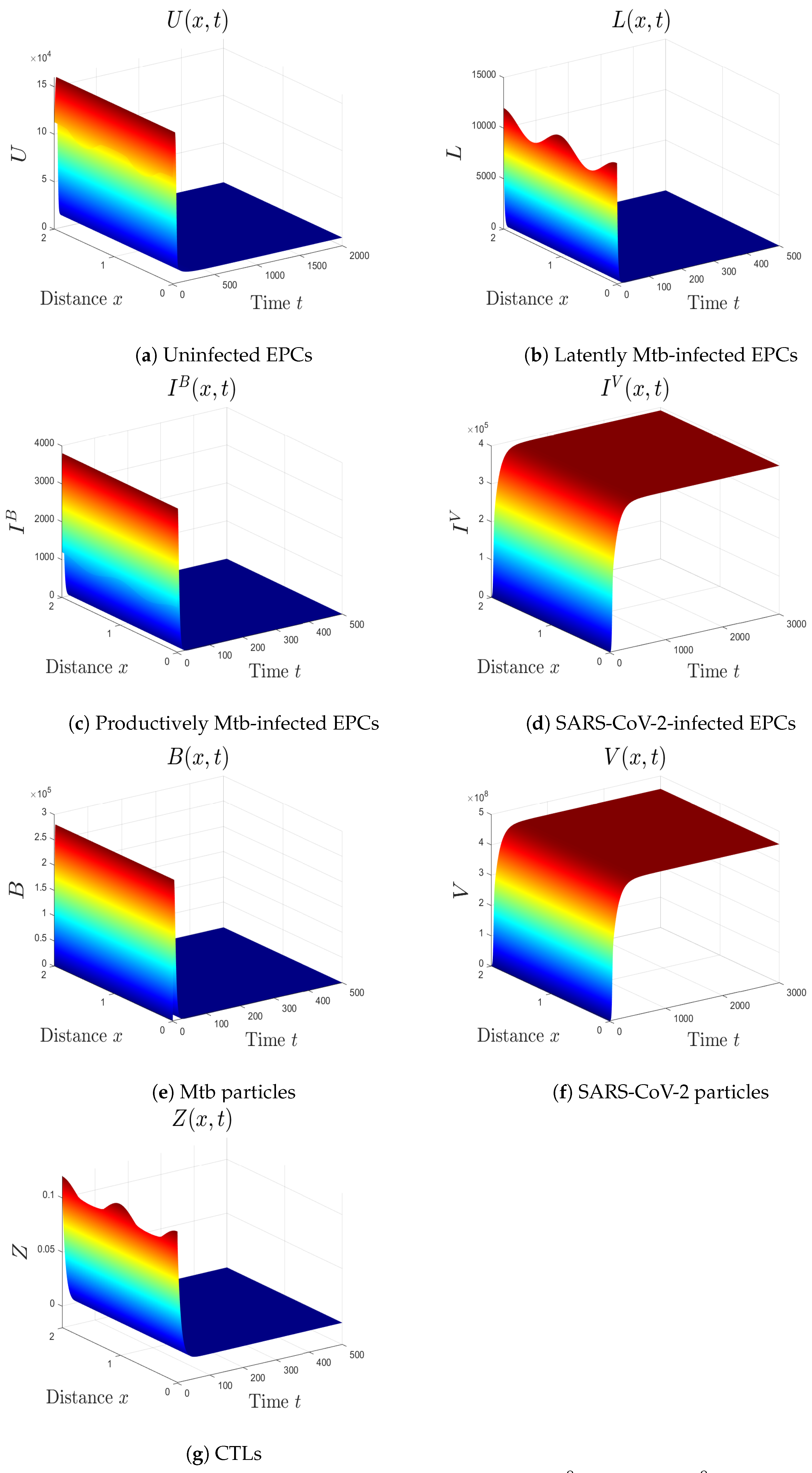
We take ${\eta }_1=2.5\times {10}^{-9}$, ${\eta }_2=1\times {10}^{-9}$, and $\omega =1\times {10}^{-8}$. We obtain ${\mathcal{R}}_{0V}=46.6667>1$, ${\displaystyle \frac{{\mathcal{R}}_{0B}}{{\mathcal{R}}_{0V}}}=0.0041<1$, and ${\mathcal{R}}_{1V}=0.04<1$. These conditions implicate the global stability of $E_2=\left(8571.43,0,0,391,429,0,4.56667\times {10}^8,0\right)$, which harmonizes with Theorem 4 (Figure 3). In this case, the patient has SARS-CoV-2 monoinfection in the absence of CTLs.

(iv)

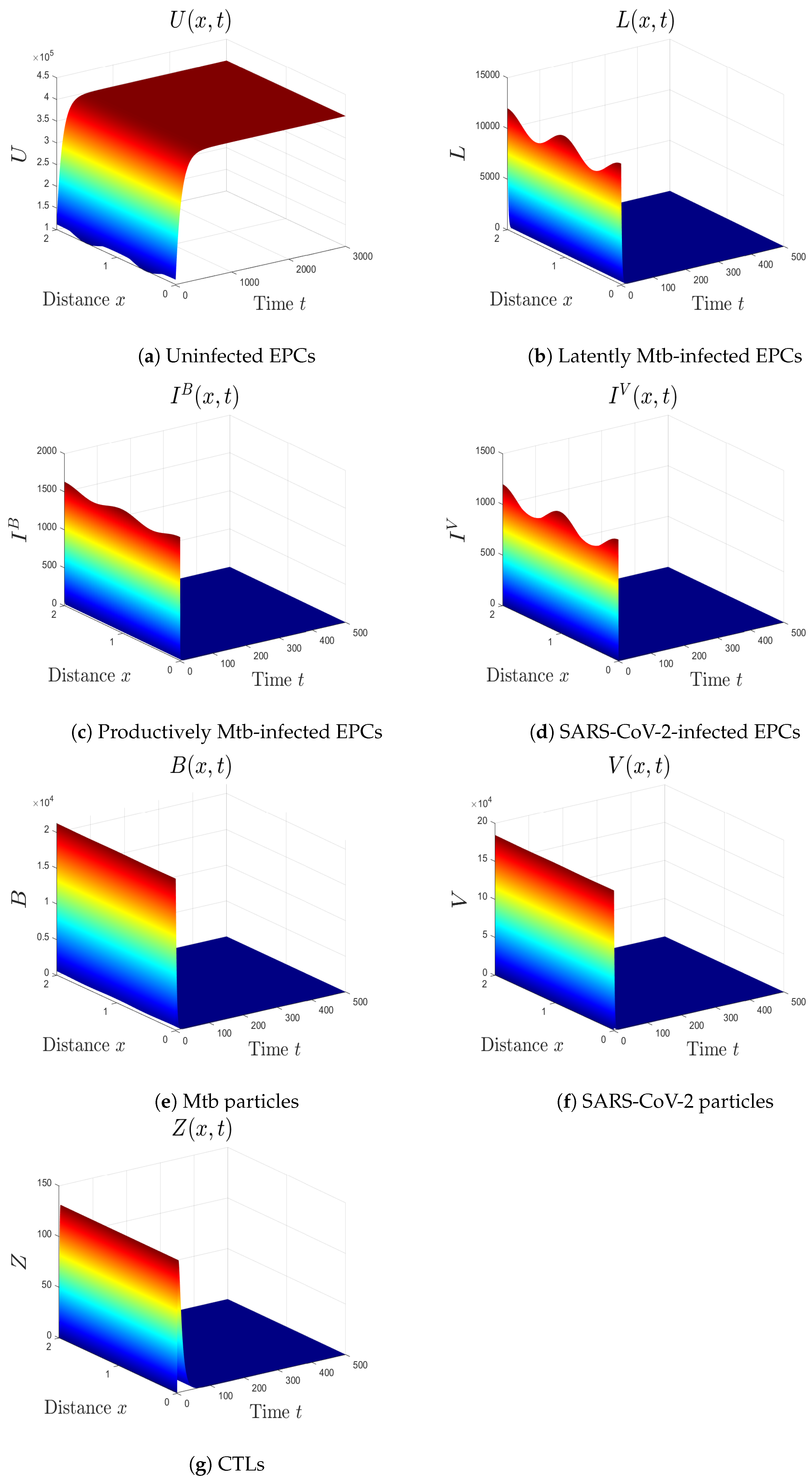
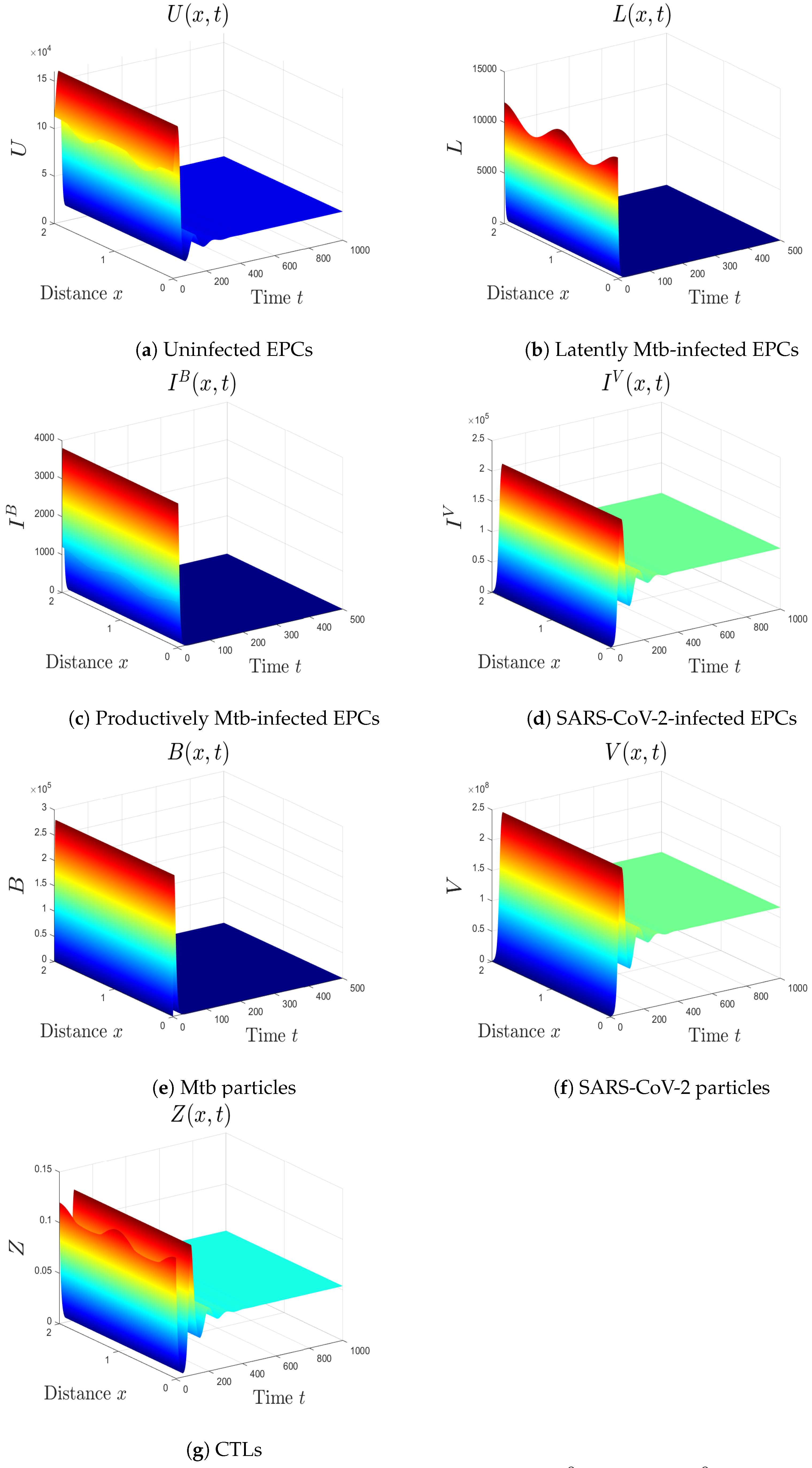
We choose ${\eta }_1=2.5\times {10}^{-7}$, ${\eta }_2=1\times {10}^{-11}$, and $\omega =1\times {10}^{-4}$. This gives ${\mathcal{R}}_{1B}=5.6497>1$ and ${\displaystyle \frac{\lambda \omega {\eta }_2{\mu }_2{ϵ}_4}{{ϵ}_2{ϵ}_5\left[\omega {ϵ}_1{ϵ}_4+{\eta }_1{\mu }_1{ϵ}_2{ϵ}_6\right]}}+1=1.0027<5.6697={\displaystyle \frac{{ϵ}_3}{{ϵ}_2}}+{\mathcal{R}}_{1B}$. This implies that the equilibrium $E_3=\left(117,514,7062.15,1000,0,96,153.8,0,4.64972\right)$ is GS (Figure 4), which comes to an agreement with Theorem 5. Here, the CTL immunity is turned on to exterminate the Mtb infection. Consequently, the densities of Mtb-infected cells and Mtb particles decrease, whilst the density of healthy cells increases.

(v)

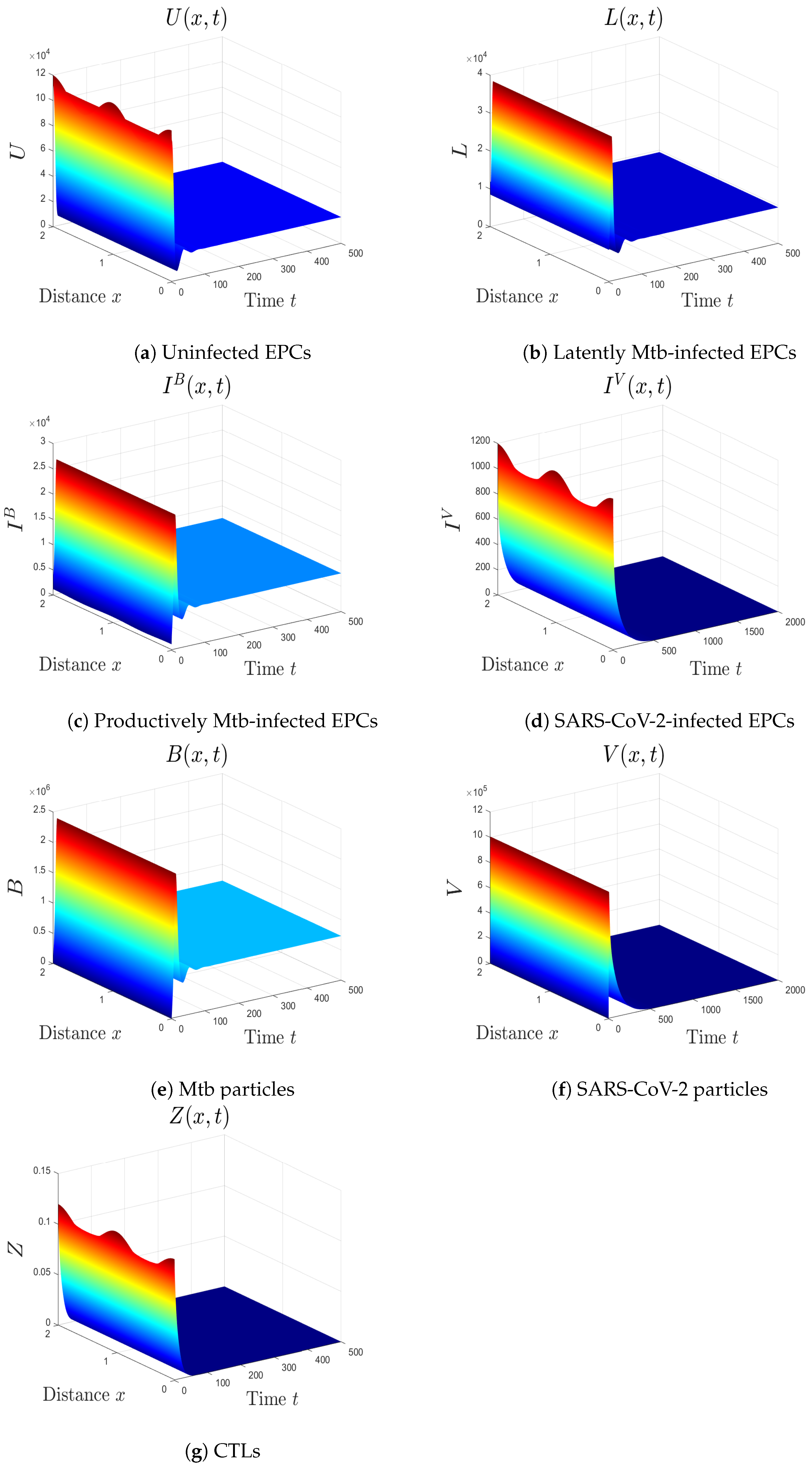
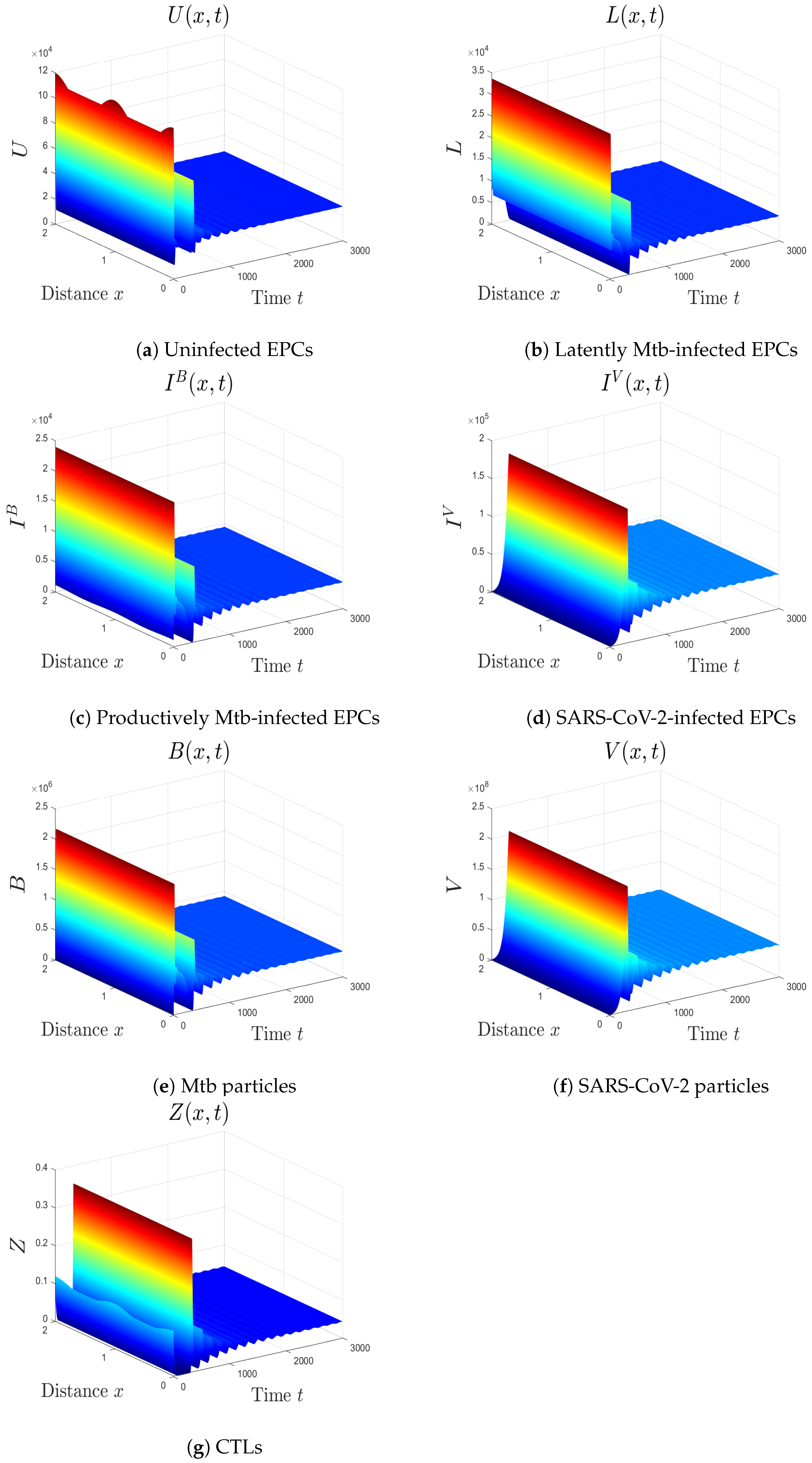
We consider ${\eta }_1=2.5\times {10}^{-9}$, ${\eta }_2=1\times {10}^{-9}$, and $\omega =1\times {10}^{-6}$. Thus, we obtain ${\mathcal{R}}_{1V}=3.6842>1$ and ${\displaystyle \frac{\lambda \omega {\eta }_1{\mu }_1{ϵ}_2{ϵ}_5}{{ϵ}_3{ϵ}_4\left[\omega {ϵ}_1{ϵ}_5+{\eta }_2{\mu }_2{ϵ}_6\right]}}+1=1.7591<53.6842={\displaystyle \frac{{ϵ}_2}{{ϵ}_3}}+{\mathcal{R}}_{1V}$. In favor of Theorem 6, $E_4=\left(31,578.9,0,0,1\times {10}^5,0,1.16667\times {10}^8,0.05368\right)$ is GS (Figure 5). This case mimics the condition of a COVID-19 patient with active CTLs which work on removing SARS-CoV-2-infected cells.

(vi)

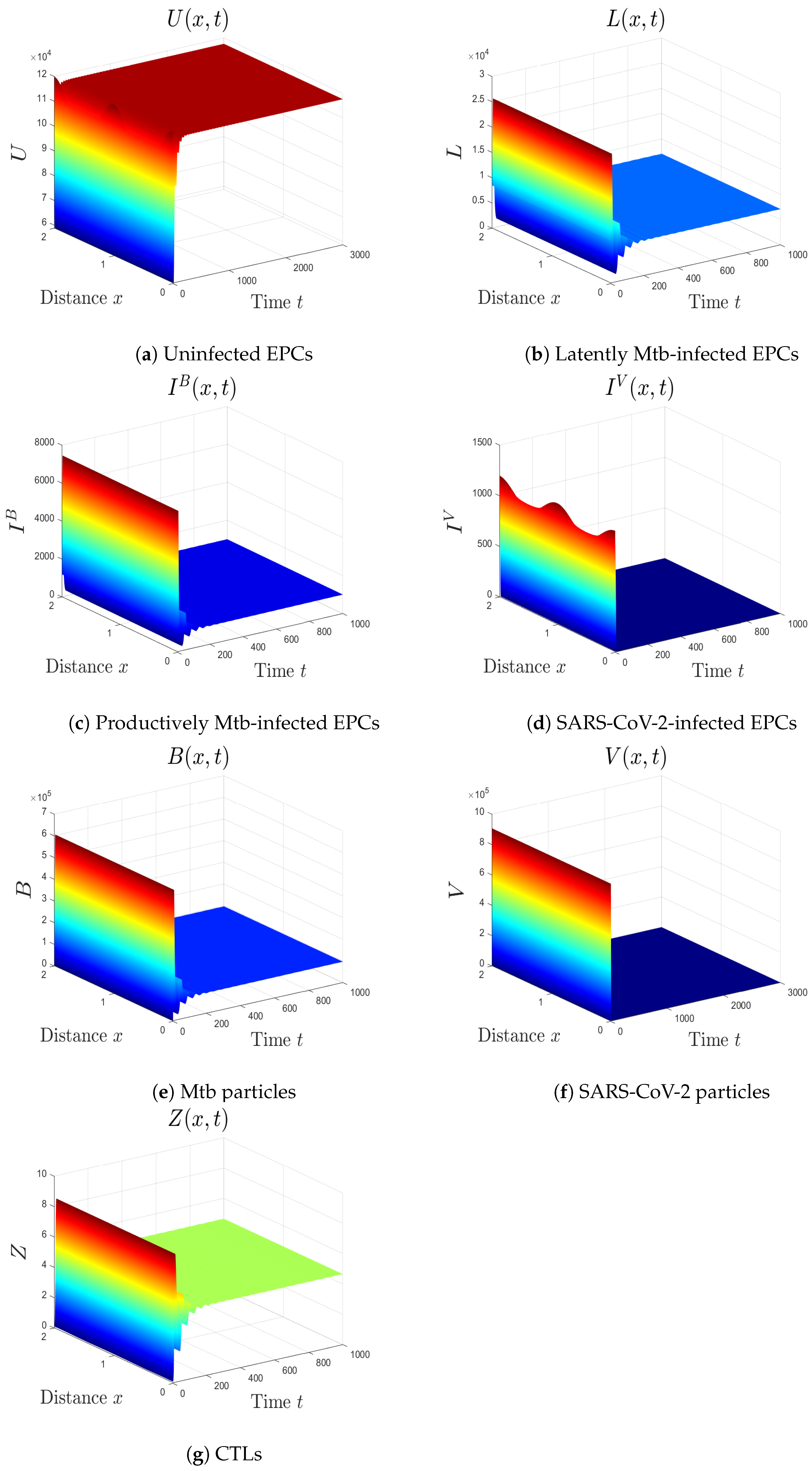
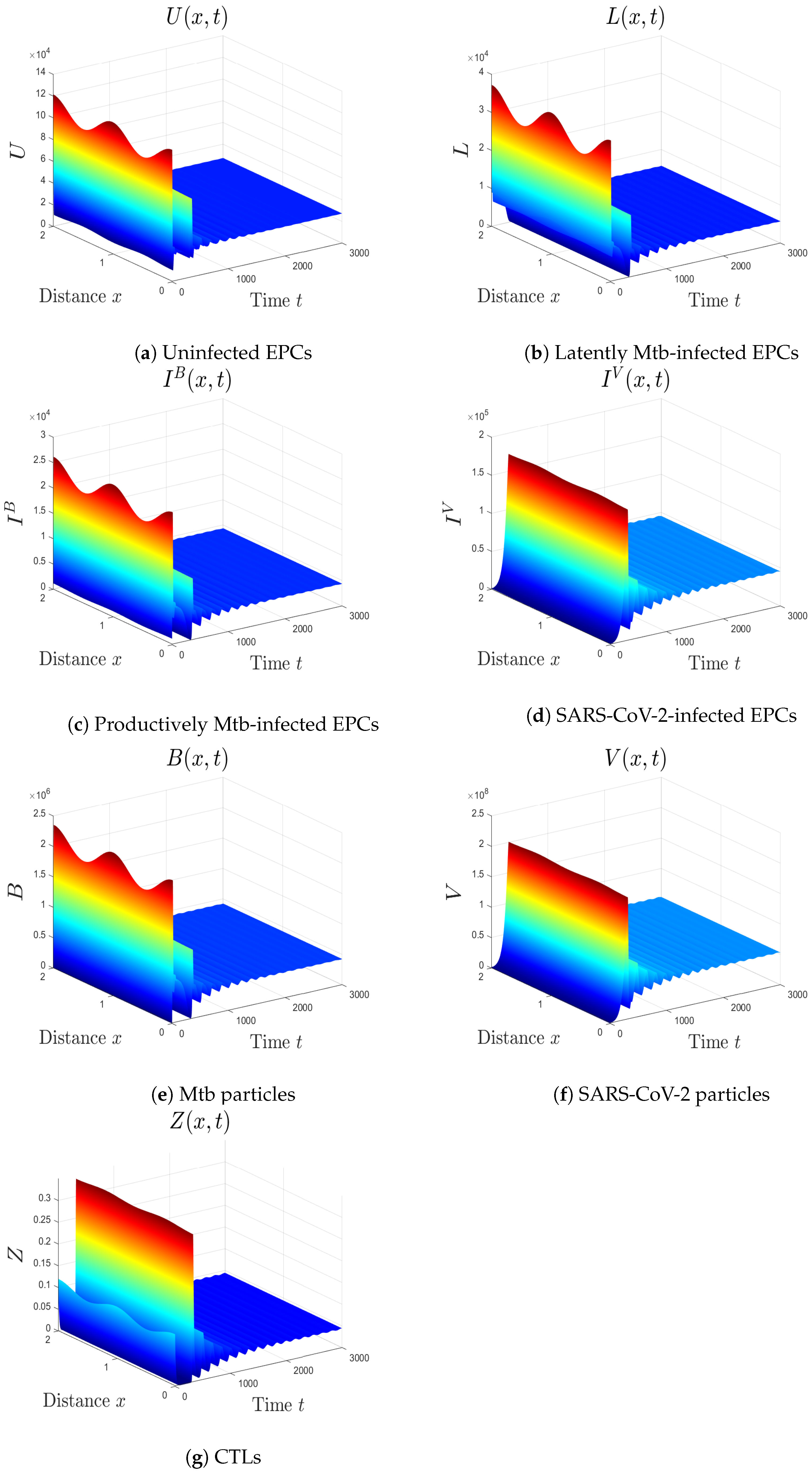
We choose ${\eta }_1=2\times {10}^{-}7$, ${\eta }_2=1\times {10}^{-9}$, and $\omega =2\times {10}^{-6}$. These values give ${\displaystyle \frac{\lambda \omega {\eta }_2{\mu }_2{ϵ}_4}{{ϵ}_2{ϵ}_5\left[\omega {ϵ}_1{ϵ}_4+{\eta }_1{\mu }_1{ϵ}_2{ϵ}_6\right]}}+1=1.0096>0.1784={\displaystyle \frac{{ϵ}_3}{{ϵ}_2}}+{\mathcal{R}}_{1B}$, ${\displaystyle \frac{\lambda \omega {\eta }_1{\mu }_1{ϵ}_2{ϵ}_5}{{ϵ}_3{ϵ}_4\left[\omega {ϵ}_1{ϵ}_5+{\eta }_2{\mu }_2{ϵ}_6\right]}}+1=113.5704>56.8293={\displaystyle \frac{{ϵ}_2}{{ϵ}_3}}+{\mathcal{R}}_{1V}$, ${\displaystyle \frac{{\mathcal{R}}_{0V}}{{\mathcal{R}}_{0B}}}=3.0333>1$, and $\sigma =16.4835>1$. This implicates the global stability of $E_5=(27,125.6,5712.6,4380.44,45,619.6,421,196$, $5.322\times {10}^7,0.043)$, which is compatible with Theorem 7 (Figure 6). In this situation, the person has SARS-CoV-2/Mtb coinfection with robust CTL immunity.

5.1. The Movement from the Monoinfection to the Coinfection State

From the results above, we see that increasing the infection rate of EPCs by SARS-CoV-2, ${\eta }_2$, forces the system to move from Mtb monoinfection state to SARS-CoV-2/Mtb coinfection state. In other words, $E_3$ loses its stability and $E_5$ becomes GS. Similarly, increasing the infection rate by Mtb, ${\eta }_1$, pushes the system from SARS-CoV-2 monoinfection state to the coinfection state. In this case, $E_4$ loses its stability and $E_5$ becomes GS. Therefore, the values of these parameters need to be controlled as they have a powerful effect in converting the system from the monoinfection zone to the coinfection zone.

5.2. The Impact of the Diffusion Coefficients On Coinfection

To test the impact of the diffusion coefficients in model (1) on the behavior of the solutions, we change the values of the coefficients considered in case (vi) to $D_U=D_L=D_{I^B}=D_{I^V}=D_B=D_V=D_Z=1\times {10}^{-5}$. We observe from Figure 7 that the effect of this change appears at the initial times, while the final solutions are not affected. Thus, the diffusion coefficients do not affect the robustness of the global stability of the solutions. Therefore, the impact of these coefficients should be monitored at the beginning of coinfection as it affects the distribution of particles in space.

6. Conclusions and Future Works

There is an emerging evidence that the COVID-19 patients who have Mtb are more likely to develop acute disease and die [2,3,8]. Therefore, understanding Mtb/SARS-CoV-2 coinfection is critical to treat this group of patients. Here, we introduced a reaction–diffusion within-host Mtb/SARS-CoV-2 model. It counts the connections between uninfected EPCs, latently Mtb-infected EPCs, productively Mtb-infected EPCs, SARS-CoV-2-infected EPCs, Mtb particles, SARS-CoV-2 virions, and CTLs. It owns six equilibrium points as the following:

(i)

The uninfected equilibrium $E_0$ constantly exists. It is GS if ${\mathcal{R}}_{0B}\le 1$ and ${\mathcal{R}}_{0V}\le 1$. This equilibrium imitates the status of a healthy individual with negative SARS-CoV-2 and Mtb tests.

(ii)

The Mtb immune-free equilibrium $E_1$ is marked if ${\mathcal{R}}_{0B}>1$, while it is GS if ${\displaystyle \frac{{\mathcal{R}}_{0V}}{{\mathcal{R}}_{0B}}}\le 1$ and ${\mathcal{R}}_{1B}\le 1$. The patient here suffers from Mtb monoinfection, where the CTL immunity has not yet been activated.

(iii)

The COVID-19 immune-free equilibrium $E_2$ occurs when ${\mathcal{R}}_{0V}>1$. It is GS if ${\displaystyle \frac{{\mathcal{R}}_{0B}}{{\mathcal{R}}_{0V}}}\le 1$ and ${\mathcal{R}}_{1V}\le 1$. Here, the patient has SARS-CoV-2 monoinfection with inefficient CTLs.

(iv)

The Mtb equilibrium with immunity $E_3$ exists if ${\mathcal{R}}_{1B}>1$, while it is GS if ${\displaystyle \frac{\lambda \omega {\eta }_2{\mu }_2{ϵ}_4}{{ϵ}_2{ϵ}_5\left[\omega {ϵ}_1{ϵ}_4+{\eta }_1{\mu }_1{ϵ}_2{ϵ}_6\right]}}+1\le {\displaystyle \frac{{ϵ}_3}{{ϵ}_2}}+{\mathcal{R}}_{1B}$. In this condition, the CTL immunity is stimulated to eliminate Mtb infection.

(v)

The COVID-19 equilibrium with immunity $E_4$ exists if ${\mathcal{R}}_{1V}>1$, and it is GS if ${\displaystyle \frac{\lambda \omega {\eta }_1{\mu }_1{ϵ}_2{ϵ}_5}{{ϵ}_3{ϵ}_4\left[\omega {ϵ}_1{ϵ}_5+{\eta }_2{\mu }_2{ϵ}_6\right]}}+1\le {\displaystyle \frac{{ϵ}_2}{{ϵ}_3}}+{\mathcal{R}}_{1V}$. This simulates the case of an individual with COVID-19 infection and active CTL immunity.

(vi)

The Mtb/SARS-CoV-2 coinfection equilibrium $E_5$ exists and it is GS if ${\displaystyle \frac{\omega \lambda {\eta }_2{\mu }_2{ϵ}_4}{{ϵ}_2{ϵ}_5\left[\omega {ϵ}_1{ϵ}_4+{\eta }_1{\mu }_1{ϵ}_2{ϵ}_6\right]}}+1>{\displaystyle \frac{{ϵ}_3}{{ϵ}_2}}+{\mathcal{R}}_{1B}$, ${\displaystyle \frac{\omega \lambda {\eta }_1{\mu }_1{ϵ}_2{ϵ}_5}{{ϵ}_3{ϵ}_4\left[\omega {ϵ}_1{ϵ}_5+{\eta }_2{\mu }_2{ϵ}_6\right]}}+1>{\displaystyle \frac{{ϵ}_2}{{ϵ}_3}}+{\mathcal{R}}_{1V}$, ${\displaystyle \frac{{\mathcal{R}}_{0V}}{{\mathcal{R}}_{0B}}}>1$, ${ϵ}_2>{ϵ}_3$, and $\sigma >1$. Here, the patient with a single infection becomes infected with both SARS-CoV-2 and Mtb.

We found that the numerical computations are quite congruous with the theoretical contributions. The equilibrium points reflect three states: the healthy state, the monoinfection state, and the coinfection state. The threshold parameters defined in Proposition 1 determine the locomotion between these states. Thus, the values of parameters in model (1) should be selected with caution. In addition, the global stability of the solutions of model (1) is robust against the values of the diffusion coefficients. However, the initial distributions of particles are affected by the selection of these values. Thus, it should be monitored as it may affect the initial status of the coinfected patients. In fact, Mtb/SARS-CoV-2 coinfection is a disease that needs to be further investigated and requires more awareness in high-TB burden regions such as India, Indonesia, and China [2]. Understanding the dynamics of coinfection will help develop new treatments, find better ways to treat coinfected patients, or recommend preventive measures for coinfected patients. The main limitation of this work is that we did not acquire real data to estimate the values of parameters in system (1). We gathered the values from SARS-CoV-2 monoinfection models or Mtb monoinfection models. Furthermore, we proved the boundedness only for the case when $D_U=D_L=D_{I^B}=D_{I^V}=D_Z$. In addition, we assumed that CTLs kill infected cells at the same rate constant. Therefore, this work could be polished by (i) utilizing real data to obtain an estimation of the values of parameters in system (1) when the data on coinfection become available, (ii) proving the boundedness for different diffusion coefficients, (iii) analyzing the model with different killing rates of CTLs, (iv) counting the time delays inherent in the latent stage or other responses, (v) adding the role of antibodies in eliminating SARS-CoV-2 or Mtb particles, (vi) using fractional derivatives to study model (1) [45,46], (vii) performing a sensitivity analysis for the threshold parameters to identify the most sensitive parameters in the model [47], (viii) considering mutations that can generate more aggressive variants of SARS-CoV-2 and their effect on coinfection dynamics [48], and (ix) developing a multiscale model to connect within-host dynamics with between-hosts dynamics and gain a better comprehension of the coinfection mechanism.

References

- Coronavirus Disease (COVID-19), Weekly Epidemiological Update (12 October 2022), World Health Organization (WHO). 2022. Available online: https://www.who.int/publications/m/item/weekly-epidemiological-update-on-covid-19---1-march-2023 (accessed on 1 January 2023).
- Song, W.; Zhao, J.; Zhang, Q.; Liu, S.; Zhu, X.; An, Q.Q.; Xu, T.T.; Li, S.J.; Liu, J.Y.; Tao, N.N.; et al. COVID-19 and Tuberculosis coinfection: An overview of case reports/case series and meta-analysis. Front. Med. 2021, 8, 657006. [Google Scholar] [CrossRef] [PubMed]
- Shah, T.; Shah, Z.; Yasmeen, N.; Baloch, Z.; Xia, X. Pathogenesis of SARS-CoV-2 and Mycobacterium tuberculosis coinfection. Front. Immunol. 2022, 13, 909011. [Google Scholar] [CrossRef] [PubMed]
- Luke, E.; Swafford, K.; Shirazi, G.; Venketaraman, V. TB and COVID-19: An exploration of the characteristics and resulting complications of co-infection. Front. Biosci. 2022, 14, 6. [Google Scholar] [CrossRef] [PubMed]
- Gatechompol, S.; Avihingsanon, A.; Putcharoen, O.; Ruxrungtham, K.; Kuritzkes, D.R. COVID-19 and HIV infection co-pandemics and their impact: A review of the literature. AIDS Res. Ther. 2021, 18, 28. [Google Scholar] [CrossRef] [PubMed]
- Shariq, M.; Sheikh, J.; Quadir, N.; Sharma, N.; Hasnain, S.; Ehtesham, N. COVID-19 and tuberculosis: The double whammy of respiratory pathogens. Eur. Respir. Rev. 2022, 31, 210264. [Google Scholar] [CrossRef]
- Tapela, K.; Olwal, C.O.; Quaye, O. Parallels in the pathogenesis of SARS-CoV-2 and M. tuberculosis: A synergistic or antagonistic alliance? Future Microbiol. 2020, 15, 1691–1695. [Google Scholar] [CrossRef] [PubMed]
- Petrone, L.; Petruccioli, E.; Vanini, V.; Cuzzi, G.; Gualano, G.; Vittozzi, P.; Nicastri, E.; Maffongelli, G.; Grifoni, A.; Sette, A.; et al. Coinfection of tuberculosis and COVID-19 limits the ability to in vitro respond to SARS-CoV-2. Int. J. Infect. Dis. 2021, 113, S82–S87. [Google Scholar] [CrossRef]
- Liang, K. Mathematical model of infection kinetics and its analysis for COVID-19, SARS and MERS. Infect. Genet. Evol. 2020, 82, 104306. [Google Scholar] [CrossRef] [PubMed]
- Krishna, M.V. Mathematical modelling on diffusion and control of COVID–19. Infect. Dis. Model. 2020, 5, 588–597. [Google Scholar] [CrossRef]
- Ivorra, B.; Ferrández, M.R.; Vela-Pérez, M.; Ramos, A.M. Mathematical modeling of the spread of the coronavirus disease 2019 (COVID-19) taking into account the undetected infections. The case of China. Commun. Nonlinear Sci. Numer. Simul. 2020, 88, 105303. [Google Scholar] [CrossRef]
- Yang, C.; Wang, J. A mathematical model for the novel coronavirus epidemic in Wuhan, China. Math. Biosci. Eng. 2020, 17, 2708–2724. [Google Scholar] [CrossRef] [PubMed]
- Krishna, M.V.; Prakash, J. Mathematical modelling on phase based transmissibility of Coronavirus. Infect. Dis. Model. 2020, 5, 375–385. [Google Scholar] [CrossRef] [PubMed]
- Rajagopal, K.; Hasanzadeh, N.; Parastesh, F.; Hamarash, I.I.; Jafari, S.; Hussain, I. A fractional-order model for the novel coronavirus (COVID-19) outbreak. Nonlinear Dyn. 2020, 101, 711–718. [Google Scholar] [CrossRef] [PubMed]
- Chen, T.M.; Rui, J.; Wang, Q.P.; Zhao, Z.Y.; Cui, J.A.; Yin, L. A mathematical model for simulating the phase-based transmissibility of a novel coronavirus. Infect. Dis. Poverty 2020, 9, 24. [Google Scholar] [CrossRef]
- Almocera, A.S.; Quiroz, G.; Hernandez-Vargas, E.A. Stability analysis in COVID-19 within-host model with immune response. Commun. Nonlinear Sci. Numer. 2020, 95, 105584. [Google Scholar] [CrossRef]
- Hernandez-Vargas, E.A.; Velasco-Hernandez, J.X. In-host mathematical modeling of COVID-19 in humans. Annu. Control 2020, 50, 448–456. [Google Scholar] [CrossRef]
- Li, C.; Xu, J.; Liu, J.; Zhou, Y. The within-host viral kinetics of SARS-CoV-2. Math. Biosci. Eng. 2020, 17, 2853–2861. [Google Scholar] [CrossRef]
- Blower, S.M.; Mclean, A.R.; Porco, T.C.; Small, P.M.; Hopewell, P.C.; Sanchez, M.A.; Moss, A.R. The intrinsic transmission dynamics of tuberculosis epidemics. Nat. Med. 1995, 1, 815–821. [Google Scholar] [CrossRef]
- Castillo-Chavez, C.; Feng, Z. To treat or not to treat: The case of tuberculosis. J. Math. Biol. 1997, 35, 629–656. [Google Scholar] [CrossRef]
- Feng, Z.; Castillo-Chavez, C.; Capurro, A. A model for tuberculosis with exogenous reinfection. Theor. Popul. Biol. 2000, 57, 235–247. [Google Scholar] [CrossRef]
- Castillo-Chavez, C.; Song, B. Dynamical models of tuberculosis and their applications. Math. Biosci. Eng. 2004, 1, 361–404. [Google Scholar] [CrossRef] [PubMed]
- Du, Y.; Wu, J.; Heffernan, J. A simple in-host model for Mycobacterium tuberculosis that captures all infection outcomes. Math. Popul. Stud. 2017, 24, 37–63. [Google Scholar] [CrossRef]
- He, D.; Wang, Q.; Lo, W. Mathematical analysis of macrophage-bacteria interaction in tuberculosis infection. Discret. Contin. Dyn. Syst. Ser. B 2018, 23, 3387–3413. [Google Scholar] [CrossRef]
- Yao, M.; Zhang, Y.; Wang, W. Bifurcation analysis for an in-host Mycobacterium tuberculosis model. Discret. Contin. Dyn. Syst. Ser. B 2021, 26, 2299–2322. [Google Scholar] [CrossRef]
- Zhang, W. Analysis of an in-host tuberculosis model for disease control. Appl. Math. Lett. 2020, 99, 105983. [Google Scholar] [CrossRef]
- Ibargüen-Mondragón, E.; Esteva, L.; Burbano-Rosero, E. Mathematical model for the growth of Mycobacterium tuberculosis in the granuloma. Math. Biosci. Eng. 2018, 15, 407–428. [Google Scholar] [PubMed]
- Pinky, L.; Dobrovolny, H.M. SARS-CoV-2 coinfections: Could influenza and the common cold be beneficial? J. Med. Virol. 2020, 92, 2623–2630. [Google Scholar] [CrossRef]
- Agha, A.D.A.; Elaiw, A.M. Global dynamics of SARS-CoV-2/malaria model with antibody immune response. Math. Biosci. Eng. 2022, 19, 8380–8410. [Google Scholar] [CrossRef]
- Elaiw, A.M.; Agha, A.D.A.; Azoz, S.A.; Ramadan, E. Global analysis of within-host SARS-CoV-2/HIV coinfection model with latency. Eur. Phys. J. Plus 2022, 137, 174. [Google Scholar] [CrossRef]
- Elaiw, A.M.; Agha, A.D.A. Global dynamics of SARS-CoV-2/cancer model with immune responses. Appl. Math. Comput. 2021, 408, 126364. [Google Scholar] [CrossRef]
- Mekonen, K.; Balcha, S.; Obsu, L.; Hassen, A. Mathematical modeling and analysis of TB and COVID-19 coinfection. J. Appl. Math. 2022, 2022, 2449710. [Google Scholar] [CrossRef]
- Bandekar, S.; Ghosh, M. A co-infection model on TB—COVID-19 with optimal control and sensitivity analysis. Math. Comput. Simul. 2022, 200, 1–31. [Google Scholar] [CrossRef] [PubMed]
- Marimuthu, Y.; Nagappa, B.; Sharma, N.; Basu, S.; Chopra, K. COVID-19 and tuberculosis: A mathematical model based forecasting in Delhi, India. Indian J. Tuberc. 2020, 67, 177–181. [Google Scholar] [CrossRef] [PubMed]
- Elaiw, A.M.; Agha, A.D.A. Analysis of the in-host dynamics of tuberculosis and SARS-CoV-2 coinfection. Mathematics 2023, 11, 1104. [Google Scholar] [CrossRef]
- Zhang, Y.; Xu, Z. Dynamics of a diffusive HBV model with delayed Beddington-DeAngelis response. Nonlinear Anal. Real World Appl. 2014, 15, 118–139. [Google Scholar] [CrossRef]
- Xu, Z.; Xu, Y. Stability of a CD4+ T cell viral infection model with diffusion. Int. J. Biomath. 2018, 11, 1–16. [Google Scholar] [CrossRef]
- Protter, M.H.; Weinberger, H.F. Maximum Principles in Differential Equations; Prentic Hall: Englewood Cliffs, NJ, USA, 1967. [Google Scholar]
- Henry, D. Geometric Theory of Semilinear Parabolic Equations; Springer: New York, NY, USA, 1993. [Google Scholar]
- Korobeinikov, A. Global properties of basic virus dynamics models. Bull. Math. Biol. 2004, 66, 879–883. [Google Scholar] [CrossRef]
- Roy, P.; Roy, A.; Khailov, E.; Basir, F.A.; Grigorieva, E. A model of the optimal immunotherapy of psoriasis by introducing IL-10 and IL-22 inhibitor. J. Biol. Syst. 2020, 28, 609–639. [Google Scholar] [CrossRef]
- Cao, X.; Roy, A.; Basir, F.A.; Roy, P. Global dynamics of HIV infection with two disease transmission routes—A mathematical model. Commun. Math. Biol. Neurosci. 2020, 2020, 8. [Google Scholar]
- Khalil, H.K. Nonlinear Systems; Prentice-Hall: Hoboken, NJ, USA, 1996. [Google Scholar]
- Sumi, T.; Harada, K. Immune response to SARS-CoV-2 in severe disease and long COVID-19. iScience 2022, 25, 104723. [Google Scholar] [CrossRef]
- Ain, Q.T.; Chu, Y. On fractal fractional hepatitis B epidemic model with modified vaccination effects. Fractals 2022, 1–18. [Google Scholar] [CrossRef]
- Ain, Q.T.; Anjum, N.; Din, A.; Zeb, A.; Djilali, S.; Khan, Z. On the analysis of Caputo fractional order dynamics of Middle East Lungs Coronavirus (MERS-CoV) model. Alex. Eng. J. 2022, 61, 5123–5131. [Google Scholar]
- Elaiw, A.M.; Agha, A.D.A. Global stability of a reaction-diffusion malaria/COVID-19 coinfection dynamics model. Mathematics 2022, 10, 4390. [Google Scholar] [CrossRef]
- Bellomo, N.; Burini, D.; Outada, N. Multiscale models of Covid-19 with mutations and variants. Netw. Heterog. Media 2022, 17, 293–310. [Google Scholar] [CrossRef]
Disclaimer/Publisher’s Note: The statements, opinions and data contained in all publications are solely those of the individual author(s) and contributor(s) and not of MDPI and/or the editor(s). MDPI and/or the editor(s) disclaim responsibility for any injury to people or property resulting from any ideas, methods, instructions or products referred to in the content. |
© 2023 by the authors. Licensee MDPI, Basel, Switzerland. This article is an open access article distributed under the terms and conditions of the Creative Commons Attribution (CC BY) license (https://creativecommons.org/licenses/by/4.0/).
Share and Cite
Algarni, A.; Al Agha, A.D.; Fayomi, A.; Al Garalleh, H. Kinetics of a Reaction-Diffusion Mtb/SARS-CoV-2 Coinfection Model with Immunity. Mathematics 2023, 11, 1715. https://doi.org/10.3390/math11071715
Algarni A, Al Agha AD, Fayomi A, Al Garalleh H. Kinetics of a Reaction-Diffusion Mtb/SARS-CoV-2 Coinfection Model with Immunity. Mathematics. 2023; 11(7):1715. https://doi.org/10.3390/math11071715
Chicago/Turabian StyleAlgarni, Ali, Afnan D. Al Agha, Aisha Fayomi, and Hakim Al Garalleh. 2023. "Kinetics of a Reaction-Diffusion Mtb/SARS-CoV-2 Coinfection Model with Immunity" Mathematics 11, no. 7: 1715. https://doi.org/10.3390/math11071715
APA StyleAlgarni, A., Al Agha, A. D., Fayomi, A., & Al Garalleh, H. (2023). Kinetics of a Reaction-Diffusion Mtb/SARS-CoV-2 Coinfection Model with Immunity. Mathematics, 11(7), 1715. https://doi.org/10.3390/math11071715