Article

Streamline Diffusion Finite Element Method for Singularly Perturbed 1D-Parabolic Convection Diffusion Differential Equations with Line Discontinuous Source

by
R. Soundararajan
1,2,
V. Subburayan
2,* and
Patricia J. Y. Wong
3
1
Department of Mathematics, RKM Vivekananda College (Autonomous), Mylapore, Chennai 600004, India
2
Department of Mathematics, Faculty of Engineering and Technology, SRM Institute of Science and Technology, Kattankulathur 603203, India
3
School of Electrical and Electronic Engineering, Nanyang Technological University, 50 Nanyang Avenue, Singapore 639798, Singapore
*
Author to whom correspondence should be addressed.
Mathematics 2023, 11(9), 2034; https://doi.org/10.3390/math11092034
Submission received: 22 March 2023 / Revised: 21 April 2023 / Accepted: 24 April 2023 / Published: 25 April 2023
(This article belongs to the Special Issue Applications of Partial Differential Equations)

Abstract

:
This article presents a study on singularly perturbed 1D parabolic Dirichlet’s type differential equations with discontinuous source terms on an interior line. The time derivative is discretized using the Euler backward method, followed by the application of the streamline–diffusion finite element method (SDFEM) to solve locally one-dimensional stationary problems on a Shishkin mesh. Our proposed method is shown to achieve first-order convergence in time and second-order convergence in space. Our proposed method offers several advantages over existing techniques, including more accurate approximations of the solution on the boundary layer region, better efficiency, and robustness in dealing with discontinuous line source terms. The numerical examples presented in this paper demonstrate the effectiveness and efficiency of our method, which has practical applications in various fields, such as engineering and applied mathematics. Overall, our proposed method provides an effective and efficient solution to the challenging problem of solving singularly perturbed parabolic differential equations with discontinuous line source terms, making it a valuable tool for researchers and practitioners in various domains.

1. Introduction

In the literature, there are several articles available that deal with the numerical solution of singularly perturbed 1D parabolic differential equations with sufficiently smooth data functions, see [1,2,3,4,5]. Such problems, but with non-smooth data functions, can be seen in [6,7,8]. In [9], Clavero considered a numerical scheme with two small parameters in both the convection and diffusion terms. In [10], Gracia and O’Riordan considered a singularly perturbed reaction–diffusion parabolic problem with an initial condition that was not smooth. In [11], Clavero and Jorge considered 1D singularly perturbed parabolic convection diffusion systems and used a splitting uniformly convergent method. In [12], Yao Cheng, Yanjie Mei and H G Roos considered the local discontinuous Glerkin method for time dependent singularly perturbed convection diffusion problems on layer adapted meshes.
While there have been several studies on solving parabolic differential equations with various boundary conditions, such as Dirichlet and Neumann conditions, the problem of nonlinear parabolic stochastic differential equations with nonlinear Robin conditions remains an active area of research. For instance, the recent article, [13], discusses Well-Posedness for Nonlinear Parabolic Stochastic Differential Equations with Nonlinear Robin Conditions which provides a rigorous analysis of the mathematical properties of this problem. In this study, we focus on the related, but distinct, problem of numerically solving 1D singularly perturbed parabolic differential equations with discontinuous source terms on an interior line.
This type of problem has a regular boundary layer at x = 1 (boundary point) as the parameter ε tends to zero [14]. As a layer near the boundary exists, conventional discretization techniques, such as Finite Difference Methods (FDMs) or Finite Element Methods (FEMs), cannot yield an accurate solution, unless the mesh is highly refined [14]. Therefore, it is essential that any method proposed must employ a layer-adapted mesh to achieve uniform accuracy. Mukherjee and Natesan [15] developed a hybrid finite difference approach that converges uniformly for singularly perturbed 1D parabolic initial-boundary value problems (IBVPs) on the piecewise uniform Shishkin mesh. Similarly, Das et al. [16] proposed a numerical technique on the Bakhvalov-Shishkin mesh to solve 2D delay parabolic IBVPs. Hughes and Brooks [17] introduced the Streamline–diffusion finite element method (SDFEM), which is widely recognized as an effective technique for obtaining the numerical solutions of convection-dominated flow problems. Later, Roos and Zarin [18] applied SDFEM on the Shishkin mesh to solve a singularly perturbed two-point boundary value problem with a non-smooth source function.
The main focus of this paper was to investigate the numerical treatment of 1D singularly perturbed parabolic Dirichlet’s differential equations with discontinuous source terms on an interior line. This problem contains an interior layer at x = z due to the presence of line discontinuities. The authors propose a method that first uses the backward Euler method to discretize the time derivative, followed by applying SDFEM on the Shishkin mesh to solve the locally one-dimensional stationary problem. In [19], Ghiocel Groza and Nicolae Pop considered a numerical scheme for the locally one-dimensional stationary boundary value problem. Various numerical examples were used to validate the suggested method, both theoretically and numerically, and it demonstrated uniform convergence in both space and time.
The paper is organized as follows: Section 2 presents the statement of the problem, the temporal discretization, derivative estimates and stability findings of locally 1D problems. In Section 3 and Section 4, the weak formulation and the numerical scheme for solving our problem are described. In Section 5, the error estimate for the SDFEM method is provided, while Section 6 offers numerical validation through various test examples. Finally, Section 7 provides some concluding remarks.

2. Continuous Problem and Stability Analysis

2.1. Statement of Continuous Problem

Inspired by the work of [20], the following singularly perturbed 1D parabolic differential equation is investigated in this paper.
Find a function u such that
M u : = u t ε u x x + a ( x ) u x + b ( x ) u = δ ( x z ) g ( t ) + f ( x , t ) , ( x , t ) Ω * × ( 0 , T ] ,
u ( x , 0 ) = u 0 ( x ) , x Ω ,
u ( 0 , t ) = 0 = u ( 1 , t ) , t [ 0 , T ] ,
where 0 < ε 1 is a very small positive parameter, Ω * = Ω Ω + , Ω = ( 0 , z ) , Ω + = ( z , 1 ) , Ω ¯ = [ 0 , 1 ] , the functions a ( x ) α > 0 , b ( x ) > β > 0 , g ( t ) , f ( x , t ) and u 0 ( x ) are sufficiently differentiable and bounded in their respective domains, δ ( x z ) is the delta function, and T is some fixed positive time.
In [18], Roos and Zarin used the SDFEM method to solve a two-point boundary value problem with a point source function, which exhibits singular perturbation and requires a layer adaptive mesh like Shishkin mesh. In their model, there was only one interior layer at a single point. However, in our problem, which involves time evolution, we have an interior layer along a line source. Thus, we need to accurately capture the numerical solution along this line source.
In the paper, the positive constant C is used to denote a generic constant that is not dependent on the perturbation parameter ε , or the discretization parameters, such as N or M. For practical purposes, the accepted convention is to assume ε C N 1 for the convection coefficient problem. Additionally, the authors use the supremum norm | ψ | D = sup x D | ψ ( x ) | to measure the error and derivative bounds.

2.2. Time Domain Discretization and Locally 1D Problems

We introduce equidistant meshes in the time domain [ 0 , T ] with time step Δ t , such that Ω t M = { t i = i Δ t } i = 0 M , Δ t = T M , where M represents the number of mesh elements in the time direction. Now, discretizing the time derivative by means of the Euler fractional method on uniform mesh, we obtain the following ordinary differential equation for every time step t n in the set Ω t M , where n ranges from 1 to M:
( I + Δ t L ) u ˜ n = u ˜ n 1 + Δ t [ f ( x , t n ) + δ ( x z ) g ( t n ) ] , x Ω *
u ˜ n ( 0 ) = 0 = u ˜ n ( 1 ) ,
where the differential operator L = ε d 2 d x 2 + a ( x ) d d x + b ( x ) and u ˜ n is the solution of (4) and (5). Note that u ˜ 0 ( x ) = 0 = u 0 ( x ) , x Ω ¯ .
To achieve the stability of the scheme given by (4) and (5), one can easily prove that the operator Q = ( I + Δ t L ) satisfies the maximum principle:
Q 1 1 1 + β Δ t .
We can rewrite the semi-discretized problem (4) and (5) as:
L * u ˜ n : = ε d 2 u ˜ n ( x ) d 2 x + a ( x ) d u ˜ n ( x ) d x + c ( x ) u ˜ n ( x ) = g n ( x ) , x Ω * , u ˜ n ( 0 ) = 0 = u ˜ n ( 1 )
where c ( x ) = b ( x ) + 1 Δ t and g n ( x ) = 1 Δ t u ˜ n 1 + { f ( x , t n ) + δ ( x z ) g ( t n ) } . The above scheme (7) is an ordinary differential equation in space variable x for each time step t n .

2.3. Maximum Principle and Derivative Estimates

Lemma 1
(Maximum Principle). Suppose that there exists a function ξ, belonging to the set C 0 ( Ω ¯ ) C 2 ( Ω * ) , that satisfies the following conditions: ξ ( x ) 0 for x = 0 , 1 ,   L * ξ ( x ) 0 for all x Ω * and ξ ( z ) ξ ( z + ) 0 Then, it can be concluded that ξ ( x ) 0 for all x Ω ¯ .
Proof. 
The method of proof for the lemma is comparable to the one used in (Lemma 2 in [21]). □
Lemma 2.
Suppose u ˜ n is the solution of problem (7) and is decomposed as u ˜ n = r + s . Then, the derivatives of the regular components satisfy
d l r ( x ) d x l Ω * C ( 1 + ε l + 2 ) , l = 0 , 1 , 2 , 3 ,
and, the derivatives of the singular components satisfy
d l s ( x ) d x l C ε l exp α ( x z ) ε , x Ω , l = 0 , 1 , 2 , 3 , exp α ( x 1 ) ε , x Ω + .
Proof. 
A similar strategy to the one used in (Theorem 9.1 in [22]) is employed for the proof. □

2.4. Truncation Error

Lemma 3.
Assume that, | i u t i | C , i = 0 , 1 , 2 , 3 , then e n C Δ t 2 and E n C Δ t , where e n = u ( x , t n ) u ¯ n and E n = j = 1 n e j .
Proof. 
As u ˜ n is the solution of (4) and (5), we have
( I + Δ t L ) u ˜ n Δ t { f ( x , t n ) + δ ( x z ) g ( t n ) } = u n 1 .
By means of Taylor expansion, we have
u ( x , t n 1 ) = u ( x , t n ) Δ t u t ( x , t n ) + O ( Δ t 2 ) .
From Equation (1) and if the solution of (1) is smooth enough, we have
u t ( x , t n ) = { f ( x , t n ) + δ ( x z ) g ( t n ) } L u n .
From (10)–(12), we have
( I + Δ t L ) e n = O ( Δ t 2 ) , e n ( 0 ) = e n ( 1 ) = 0 .
From this, we have e n C ( Δ t ) 2 by using the stability result in (6).
The stability result and consistency property of (4) and (5) together implies E n C Δ t .  □

3. Weak Formulation

The standard weak formulation of problem (7) for a fixed n is given as follows. Find u ˜ n V = H 0 1 ( Ω ¯ ) , such that
B ( u ˜ n , v ) = g n ( v ) , v V ,
where
B ( y , v ) = ε ( y , v ) + ( a y + c y , v )
g n ( v ) = ( g n , v ) .
Here, (. , .) represents the inner product in L 2 ( Ω * ) .
Consider the mesh in space as Ω ¯ x N = { x 0 , x 1 , , x N } , where N is some positive integer. We define a mesh that includes the point z as one of its nodes. Let ϕ i be the basis for the finite-dimensional subspace V h of piece-wise linear polynomials. The basis is given by
ϕ i ( x ) = x x i 1 h i x i 1 x x i , x i + 1 x h i + 1 x i x x i + 1 , 0 o t h e r w i s e ,
where h i = x i x i 1 and i { 1 , 2 , , N } . We use this basis to ensure that z is one of the mesh points.
The standard Galerkin method is given as follows: find u ˜ h n V h V = H 0 1 ( Ω ¯ ) such that
B h ( u ˜ h n , v h ) = g h n ( v h ) , v h V h .

4. Streamline Diffusion Finite Element Formulation

The streamline diffusion weak formulation for the problem (7) is to find u ˜ h n V h V = H 0 1 ( Ω ¯ ) , such that
B h ( u ˜ h n , v h ) = g h n ( v h ) , v V h ,
where
B h ( y , w ) = ε ( y , w ) + ( a y + c y , w ) + i = 1 N x i 1 x i δ i ( ε y + a y + c y ) a w d x ,
g h n ( w ) = ( g n , w ) + i = 1 N x i 1 x i δ i g n ( x ) a ( x ) w d x .
The parameter, known as the Streamline–diffusion (SD) parameter, denoted as δ i , is decided later.
The SDFEM’s relevant difference scheme is presented below.
L S D N : = ε [ D + u i D u i ] + α i D u i + β i D + u i + γ i u i = g h ( ϕ i ) ,
where the symbols D + and D are given by the following:
D + u i = u i + 1 u i h i + 1 , D u i = u i u i 1 h i ,
and
α i = x i 1 x i a ( x ) ϕ i d x h i x i 1 x i c ( x ) ϕ i 1 ϕ i d x + δ i h i x i 1 x i a ( x ) 2 d x δ i x i 1 x i a ( x ) c ( x ) ϕ i 1 d x , β i = x i x i + 1 a ( x ) ϕ i d x + h i + 1 x i x i + 1 c ( x ) ϕ i + 1 ϕ i d x δ i + 1 h i + i x i x i + 1 a ( x ) 2 d x δ i + 1 x i x i + 1 a ( x ) c ( x ) ϕ i + 1 d x , γ i = x i 1 x i + 1 c ( x ) ϕ i d x + δ i h i x i 1 x i a ( x ) c ( x ) d x δ i + 1 h i + 1 x i x i + 1 a ( x ) c ( x ) d x .
The standard Galerkin method is effective for step lengths that are sufficiently small. If this condition is not met, the method can be stabilized by utilizing the characteristics of an M-matrix. To satisfy this condition, the streamline–diffusion parameter δ i can be determined such that the matrix resulting from the associated difference scheme (14) transforms into an M-matrix, as outlined below:
[ α i ] δ i = 0 ε ,
This can be written as C ¯ i h i A ¯ i + ε , where A ¯ i = x i 1 x i a ( x ) ϕ i d x and C ¯ i = x i 1 x i c ( x ) ϕ i 1 ϕ i d x . If this condition is not met, α i is set to zero for i { 1 , 2 , , N } to achieve an M-matrix, which results in the following:
δ i = ( h i C ¯ i A ¯ i ) h i A 2 ¯ i h i A C ¯ i
where, A 2 ¯ i = x i 1 x i ( a ( x ) ) 2 d x and A C ¯ i = x i 1 x i a ( x ) c ( x ) ϕ i 1 d x . If we summarize the above conditions, then we obtain
δ i = 0 , i f C ¯ i h i A ¯ i + ε ( h i C ¯ i A ¯ i ) h i A 2 ¯ i h i A C ¯ i , o t h e r w i s e .
As a result, it is evident that δ i = O ( h i ) . By choosing v h as ϕ i as well as u ˜ h = ( u ˜ h n ( x 1 ) , u ˜ h n ( x 2 ) , , u ˜ h n ( x N ) ) R N , we obtain the linear system of algebraic equations associated with the SDFEM scheme
K u ˜ h = g h ,
where K represents a tridiagonal matrix K = ( k i j ) and g h = g h n ( ϕ i ) . Upon computing the coefficients,
k i , i 1 = ε h i 1 h i 1 x i 1 x i a ( x ) ϕ i d x + x i 1 x i c ( x ) ϕ i 1 ϕ i d x δ i h i 2 x i 1 x i a ( x ) 2 d x + δ i h i 1 x i 1 x i a ( x ) c ( x ) ϕ i 1 d x , k i , i = ε h i 1 + ε h i + 1 1 + h i 1 x i 1 x i a ( x ) ϕ i d x h i + 1 1 x i x i + 1 c ( x ) ϕ i d x + x i 1 x i c ( x ) ϕ i 2 d x + x i x i + 1 c ( x ) ϕ i 2 d x + δ i h i 2 x i 1 x i a ( x ) 2 d x + δ i + 1 h i + 1 2 x i x i + 1 a ( x ) 2 d x + δ i h i 1 x i 1 x i a ( x ) c ( x ) ϕ i d x δ i + 1 h i + 1 1 x i x i + 1 a ( x ) c ( x ) ϕ i d x k i , i + 1 = ε h i + 1 1 + h i + 1 1 x i x i + 1 a ( x ) ϕ i d x + x i x i + 1 c ( x ) ϕ i + 1 ϕ i d x δ i + 1 h i + 1 2 x i x i + 1 a ( x ) 2 d x δ i + 1 h i + 1 1 x i x i + 1 a ( x ) c ( x ) ϕ i + 1 d x .
Remark 1.
We defined the SD parameter using the procedure given in [23]. Realistically, the conventional Galerkin method satisfies the criterion that defines an M-matrix for almost all 1D problems. In such a situation, the Galerkin method and the SDFEM both yield almost identical outcomes.
Remark 2.
Generally, the conventional Galerkin method is analogous to the central finite difference approach. However, in regions where convection is dominant, applying a central finite difference approximation to the convective term may lead to oscillations [14]. In such instances, the SDFEM is a superior alternative.

4.1. Discrete Green’s Function and Stability

To establish the ( l , w 1 , ) stability of the SDFEM, we introduce the discrete Green’s function. The i-th discrete Green’s function, denoted as λ i V h , is determined by solving the following problem:
B h ( ϕ j , λ i ) = δ i j , λ i ( 0 ) = λ i ( 1 ) = 0 ,
where δ i j denotes the Kronecker delta. Additional details on these and related concepts can be found in references such as [24,25,26].
Lemma 4
([25]). If λ i = j = 1 N λ j i ϕ j , , then the discrete Green’s function exhibits the following conditions:
(1) 
λ j i 0 , i , j { 1 , 2 , , N } ,
(2) 
0 λ 1 i < < λ i i > λ i + 1 i > λ N i .
Lemma 5.
If we denote c 0 = min i { c i } , i = 1 , 2 , , N where c i = k i + 1 , i k i , i + 1 and λ i = j = 1 N λ j i ϕ j , then λ i i c 0 1 .
Proof. 
From (16), for any v h V h , we have
B h ( v h , λ i ) = v h ( x i ) .
Considering v h = j = 1 i ϕ j , one can derive
j = 1 N k = 1 j k j , k λ j i = 1 .
Expanding, we obtain
( k 1 , 1 + k 1 , 2 ) λ 1 i + j = 2 i ( k j , j 1 + k j , j + k j , j + 1 ) λ j i + k i + 1 , i ( λ i + 1 i λ i i ) + λ i i ( k i + 1 , i k i , i + 1 ) = 1 .
K is an M-matrix implying ( k i , i 1 + k i , i + k i , i + 1 ) 0 , for i { 2 , , N 1 } . Now, by means of Lemma 4 and k 1 , 1 > k 1 , 2 (property), we have
λ i i ( k i + 1 , i k i , i + 1 ) 1 .
This implies that
λ i i 1 ( k i + 1 , i k i , i + 1 ) = c i 1 .
So, we conclude that λ i i c 0 1 .  □
Lemma 6
([25]). The SDFEM, equipped with the streamline–diffusion parameter specified in Equation (15), is uniformly stable in the ( l , w 1 , ) norm, as demonstrated by the following result:
v h 2 c 0 max j k = j N ( K v h ) k , v h V h , j = 1 , , N .

4.2. Shishkin Type Mesh

We used a general type mesh introduced in [27] with adapted layers at the points x = z and x = 1 . Let N be a positive even integer greater than 4 and σ 1 = min { z 2 , τ 0 α ε ln N } , σ 2 = min { 1 z 2 , τ 0 α ε ln N } , τ 0 2 . Here, we considered σ 1 = σ 2 = τ 0 α ε ln N . Let Ω s = ( 0 , z σ 1 ) ( z , 1 σ 2 ) and Ω 0 = ( z σ 1 , z ) ( 1 σ 2 , 1 ) . On Ω s and Ω o , the mesh is equidistant and graded respectively. The transition points are chosen to be
x N 4 = z σ 1 , x N 2 = z , x 3 N 4 = 1 σ 2 .
We chose two mesh generating functions φ 1 and φ 2 for the particular layers:
φ 1 ( 1 4 ) = ln N , φ 1 ( 1 2 ) = 0 ,
φ 2 ( 3 4 ) = ln N , φ 2 ( 1 ) = 0 .
The nodes of the Shishkin mesh (S-mesh) are as follows:
x i = 4 i N ( z σ 1 ) i = 0 , , N 4 , z τ 0 α ε φ 1 ( t i ) i = N 4 + 1 , , N 2 , z + 4 ( 1 z σ 2 ) ( i N 2 ) N i = N 2 + 1 , , 3 N 4 , τ 0 α ε φ 2 ( t i ) + 1 i = 3 N 4 + 1 , , N ,
where t i = i N , φ i = ln ψ i for i = 1 , 2 , ψ 1 ( t ) = exp ( ( 2 4 t ) ln N ) and ψ 2 ( t ) = exp ( ( 4 4 t ) ln N ) on Shishkin mesh (S-mesh).
max i | ψ i | , i = 1, 2 plays a part in error analysis as we see in the upcoming section. we have max | ψ | C ln N in the S-mesh. Assuming that the mesh generating function φ i , for i = 1 , 2 , obeys the following:
max { | φ i | } N C 0 , f o r i = 1 , 2 .
We observe that on the coarse part Ω s , the following holds for the S-mesh:
h i N C .
On the layer part it is true that on the S-mesh,
h i C ε ln N N
and, by the assumption (18), we obtain
h i ε C N 1 max | φ | C .

5. Error Estimations

The error at each time level t n , where 1 n M 1 , can be expressed as the difference between u ˜ n ( x i ) and u ˜ h n ( x i ) for all x i Ω * . Another way to represent this error is by utilizing the linear interpolant u ˜ I n of u ˜ n as follows:
e ( x i ) = ( u ˜ n u ˜ h n ) ( x i ) = ( u ˜ n u ˜ I n ) ( x i ) + ( u ˜ I n u ˜ h n ) ( x i ) = e I + e D .
The errors of interpolation and discretization are denoted by e I and e D , respectively. In this section, we begin by deriving an estimate for the upper bound of the discretization error, based on the error caused by interpolation. Following that, we estimate the upper bound of the interpolation error.
The discretization error is given by
e D = ( u ˜ I n u ˜ h n ) ( x ) = i = 0 N e i ϕ i .
By means of the orthogonality property, we have
B h ( u ˜ n u ˜ h n , v h ) = 0 , v h V h .
Using the above property, we obtain
B h ( e D , ϕ i ) = B h ( u ˜ I n u ˜ h n , ϕ i ) = B h ( u ˜ I n u ˜ n , ϕ i ) , i { 1 , 2 , , N 1 } .
Therefore, the equation for error is
B h ( e D , ϕ i ) = B h ( u ˜ I n u ˜ n , ϕ i ) , i { 1 , 2 , , N 1 } , e 0 D = 0 , e N D = 0 .
The following lemma gives the explicit expression for B h ( u ˜ I n u ˜ n , ϕ i ) .
Lemma 7.
The error Equation (23) involves the bilinear form B h ( u ˜ I n u ˜ n , ϕ i ) , which can be explicitly expressed as follows:
B h ( u ˜ I n u ˜ n , ϕ i ) = O i + ( P i + P i + 1 ) + ( Q i Q i + 1 ) + ( R i R i + 1 ) + ( S i S i + 1 ) ,
where
O i = x i 1 x i + 1 a ( x ) ( u ˜ I n u ˜ n ) ϕ i d x ,
P i = x i 1 x i c ( x ) ( u ˜ I n u ˜ n ) ϕ i d x ,
Q i = δ i h i x i 1 x i ( a ( x ) c ( x ) ( u ˜ I n u ˜ n ) + a ( x ) 2 ( u ˜ I n u ˜ n ) ) d x ,
R i = ε δ i h i 1 x i 1 x i a ( x ) ( u ˜ I n u ˜ n ) d x ,
S i = h i 1 x i 1 x i a ( x ) ( u ˜ I n u ˜ n ) d x .
Proof. 
One can prove the required results by a simple calculation. □
Lemma 8.
Assume that a ( x ) W 2 , 1 , then the following estimates are true:
( i ) i = 1 N | O i | c 1 u ˜ n u ˜ I n , ( i i ) i = 1 N | P i | c 2 u ˜ n u ˜ I n , ( i i i ) Q i c 3 u ˜ n u ˜ I n , ( i v ) R i c 4 u ˜ n u ˜ I n , ( v ) S i c 5 u ˜ n u ˜ I n .
Proof. 
We prove this Lemma sequentially:
(i).
From (24), we know that
O i = x i 1 x i + 1 a ( x ) ( u ˜ I n u ˜ n ) ϕ i d x .
Now, taking all the intervals and summing up, we have
i = 1 N | O i | u ˜ I n u ˜ n i = 1 N x i 1 x i + 1 a ( x ) d x u ˜ I n u ˜ n | a ( x ) | 1 , 1 = c 1 u ˜ I n u ˜ n .
(ii).
From Equation (25), we have
P i = x i 1 x i c ( x ) ( u ˜ I n u ˜ n ) ϕ i d x .
If we conduct a summation over all intervals, and derive
i = 1 N | P i | u ˜ I n u ˜ n a ( x ) h i = c 2 u ˜ I n u ˜ n .
(iii).
From Equation (26), we have
Q i = δ i h i x i 1 x i ( a ( x ) c ( x ) ( u ˜ I n u ˜ n ) + a ( x ) 2 ( u ˜ I n u ˜ n ) ) d x .
If the inequality C ¯ i h i A ¯ i + ε holds, then δ i = 0 and, as a result, r i = 0 . On the other hand, if the condition is not satisfied, then we have δ i 0 . In this scenario, it can be observed that δ i = O ( h i ) , we obtain
| Q i | C a ( x ) u ˜ I n u ˜ n ( c ( x ) h i 2 | a ( x ) | 1 , 1 ) = c 3 u ˜ I n u ˜ n .
(iv).
From Equation (27), we have
R i = ε δ i h i x i 1 x i a ( x ) ( u ˜ I n u ˜ n ) d x ,
and, here also we have r i = 0 when C ¯ i h i A ¯ i + ε , and if it is not true, we have
| R i | C | a ( x ) | 2 , 1 u ˜ I n u ˜ n = c 4 u ˜ I n u ˜ n .
(v).
Now, finally from Equation (28), we have
S i = 1 h i x i 1 x i a ( x ) ( u ˜ I n u ˜ n ) d x .
Simplifying this, we obtain
| S i | a ( x ) u ˜ I n u ˜ n = c 5 u ˜ I n u ˜ n .
Lemma 9.
Consider the problem (7) and let u ˜ n be the exact solution to this problem. Furthermore, let u ˜ I n denote the interpolant of u ˜ n on a given grid and let u ˜ h n represent the approximate solution at the time level t n . Then, It follows that
u ˜ n u ˜ h n C u ˜ I n u ˜ n .
Proof. 
Using Lemmas 6 and 8, we have
u ˜ I n u ˜ h n C max i { 1 , , N } j = i N ( K ( u ˜ I n u ˜ h n ) ) j = C max i { 1 , , N } j = i N B h ( u ˜ I n u ˜ n , ϕ j ) C i = 1 N O i + 2 i = 1 N P i + max i { 1 , , N } ( Q i Q N ) + max i { 1 , , N } ( R i R N ) + C max i { 1 , , N } ( S i S N ) C i = 1 N | O i | + 2 i = 1 N | P i | + 2 ( Q i + R i + S i ) C u ˜ I n u ˜ n .
This implies that the discretization error e D given in (22) is bounded in terms of the interpolation error e I . By applying the triangle inequality, we establish the following inequality:
u ˜ n u ˜ h n C | u ˜ I n u ˜ n .
Therefore, we have successfully demonstrated the validity of this inequality. □
We now proceed to estimate the upper bound of the interpolation error for the S-mesh.
Theorem 1.
Let u ˜ n be the classical solution of the problem (7), u ˜ I n be its interpolant on a Shishkin mesh with the grid points x i as in (17) and ε C N . Then, the following holds:
u ˜ I n u ˜ n C ( N 1 ln N ) 2 , x Ω 0 , C N 2 , x Ω s .
Proof. 
We perform a separate analysis of the error due to interpolation on the domain Ω as well as Ω + .
First, consider x in the domain Ω . Let u ˜ 1 n ( x ) be the solution to the problem:
L * u ˜ 1 n ( x ) = g n ( x ) , x Ω = ( 0 , z ) , u ˜ 0 ( 0 ) = 0 , u ˜ 0 ( z ) = d .
For now, assume that d is a constant. Then, the solution u ˜ 1 n ( x ) exists and we can decompose it as a sum of two functions r 1 and s 1 , where r 1 and s 1 satisfy bounds (8) and (9). Then, we can write
u ˜ 1 n ( x ) u ˜ 1 , I n ( x ) = r 1 ( x ) r 1 , I ( x ) + s 1 ( x ) s 1 , I ( x ) .
By means of classical theory, and from (19) and (8), we have the following estimate for the interpolation error r 1 ( x ) r 1 , I ( x ) on the regular part:
| r 1 ( x ) r 1 , I ( x ) | C h i 2 max x i 1 x x i | r 1 | C h i 2 C N 2 .
For the interpolation error r 1 ( x ) r 1 , I ( x ) in the layer part, one can derive:
| r 1 ( x ) r 1 , I ( x ) | C ε 2 ( N 1 ln N ) 2 exp 2 α τ 0 ε ( x i 1 z ) C ( N 1 ln N ) 2 .
The above expression is obtained by utilizing the inequality (20), selecting the transition point σ 1 , and assuming the condition ε C N holds. Now, for the interpolation error s 1 ( x ) s 1 , I ( x ) on the regular part, we have
| s 1 ( x ) s 1 , I ( x ) | 2 | s 1 ( x ) | C max x i 1 x x i exp α ε ( z x ) C exp α ε σ 1 = C N τ 0 .
Regarding the interpolation error for the layer component, i.e., s 1 ( x ) s 1 , I ( x ) , we apply the classical theory to obtain the following:
| s 1 ( x ) s 1 , I ( x ) | C h i 2 max x i 1 x x i | s 1 | C ( N 1 ln N ) 2 max x i 1 x x i exp α ε ( z x ) C ( N 1 ln N ) 2 .
Here, we used the inequality (20), the first inequality of (9) and (21). Similarly, we can prove the case x Ω + . □
Theorem 2.
Suppose that u ( x , t ) represents the classical solution of problem (1)–(3), u ˜ h n ( x ) represents the numerical solution of the SDFEM scheme (fully discrete) (13) at the n t h time step t n . Under the conditions of Lemma 3 and Theorem 1, we have the error estimate as follows:
u ˜ h n ( x ) u ( x , t n ) C ( ( N 1 ln N ) 2 + Δ t ) , x Ω 0 , C ( N 2 + Δ t ) , x Ω s .
Proof. 
We can prove this error estimate by combining the results from Lemma 3 and Theorem 1. □

6. Numerical Validation

In order to demonstrate the accuracy of the theoretical findings, we provide two illustrative examples in this section. We employed the double mesh principle to estimate the errors and their convergence rates for the test problems, as the exact solutions are unknown. The principle involves obtaining the numerical solution Y 2 N , k / 2 ( x i n , t i ) on a grid Ω x 2 N × Ω t 2 M , where the spatial direction is divided into 2N intervals, while the temporal direction is divided into 2M intervals. The mesh Ω x 2 N × Ω t 2 M is obtained by dividing each segment of the previous mesh Ω x N × Ω t M , where the spatial direction is divided into N intervals, while the temporal direction is divided into M intervals, in two equal parts. Subsequently, we estimate the maximum point-wise error and convergence rate for each ε .
E ε N , k = max i , n Y N , k ( x i n , t n ) Y 2 N , k / 2 ( x i n , t n ) ,
D x N , k = max ε E ε N , k , r N , k = l o g 2 D x N , k D x 2 N , k / 2 .
Example 1.
We examined the one-dimensional parabolic partial differential equation with a line source, described by Equations (1)–(3). The given data for this problem were as follows:
u ( x , 0 ) = 0 , x Ω = ( 0 , 1 ) , u ( 0 , t ) = 0 , u ( 1 , t ) = 0 , t [ 0 , 1 ] , a ( x ) = x + 5 ; b ( x ) = 1 ; f ( x , t ) = x + t ; g ( t ) = 1 ; z = 1 2 .
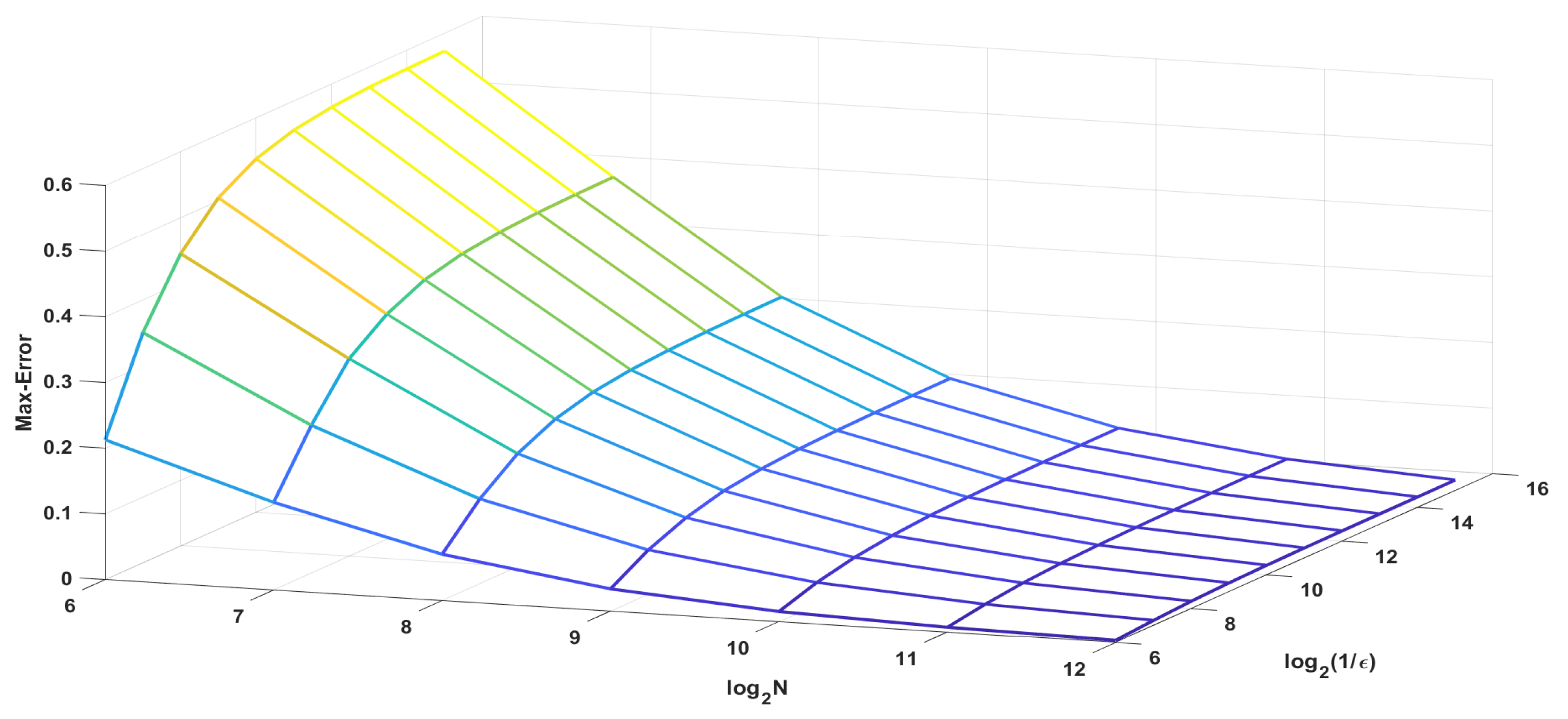
In Table 1, we list the order of convergence and the maximum point-wise error corresponding to Example 1. When M=50, the CPU run time for the error given in the table was 7.6844 × 10 2 s. Additionally, Figure 1 shows the spatial profile of the solution of the problem described in Example 1 at different times t, for a fixed value of ε and is a visual representation of the solution with a strong boundary layer at x = 1 , where the solution changed rapidly over a very small distance. This boundary layer arose due to the strong boundary condition u h n ˜ ( 1 , t ) = 0 , which forced the solution to approach the value zero very quickly. The figure also shows the location of a strong interior layer at x = 1 2 , which caused a localized increase in the solution, which arose due to the line source term at the line x = 1 2 . Figure 2 shows the corresponding point-wise maximum error, that is, the maximum error decreased as N increased, irrespective of ε .
Example 2.
We examined another one-dimensional parabolic partial differential equation with a line source, described by Equations (1)–(3). The given data for this problem were as follows:
u ( x , 0 ) = 0 , x Ω = ( 0 , 1 ) , u ( 0 , t ) = 0 , u ( 1 , t ) = 0 , t [ 0 , 1 ] , a ( x ) = 5 + x 5 + 3 x 2 + e 1 / x 2 ; b ( x ) = 1 ; f ( x , t ) = e 1 x + t ; g ( t ) = 1 ; z = 1 2 .
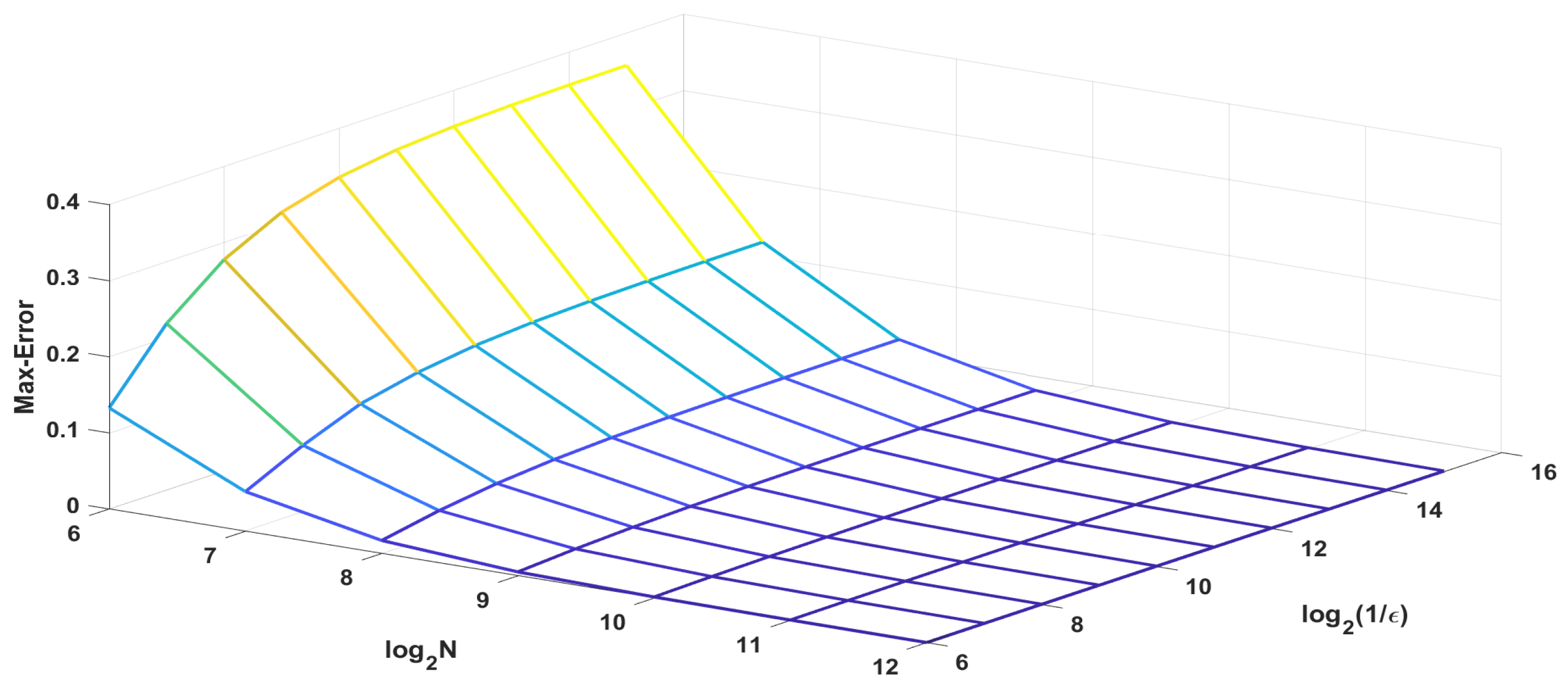
Table 2 presents the maximum point-wise error and the associated convergence rate for Example 2, when M = 50. The CPU run time for the error given in the table was 7.8426 × 10 2 s. Additionally, as illustrated in Example 1, the graphs of numerical solution and point-wise maximum error of the problem are illustrated in Figure 3 and Figure 4, respectively.
From the above two Examples, 1 and 2, we see that the solutions of the problems exhibited an interior layer at x = 1 2 and a boundary layer at x = 1 .
Note: For the numerical computation, a system with the following configuration i7 processor, 8.00 GB RAM was used.

7. Conclusions

In this study, we analyzed 1D parabolic equations that were singularly perturbed and contained a discontinuous source term on an interior line. Our objective was to discretize the time derivative using the Euler backward method and apply SDFEM to the locally one-dimensional stationary problems on Shishkin mesh. We aimed to determine the accuracy order of the spatial arrangement and evaluate test problems in terms of their maximum pointwise errors.
Our results showed that the accuracy order of the spatial arrangement was of second-order nature, but, due to the presence of the first-order term Δ t in the error bound, the overall accuracy order was limited to first-order accuracy. These findings are presented as Theorems 1 and 2. Examples 1 and 2 represent the test problems, and Figure 1 and Figure 3 depict their solutions. The layer occurred at the interior line x = z and boundary line x = 1 , which is evident from these figures. Figure 2 and Figure 4 represent the convergence of the numerical solutions, that is, they illustrate that a higher value of N corresponded to a lower maximum pointwise error.
We evaluated the test problems in terms of their maximum pointwise errors, presented in Table 1 and Table 2. From the tables we see that the computational order of convergence was almost one, but Theorem 2 showed second-order convergence in space and first-order convergence in time. This was due to the first-order term in the final result. Our results demonstrated that the maximum pointwise error stabilized as parameter ϵ decreased and decreased as parameter N increased.
It is worth noting that the results for SDFEM for ordinary differential equations, together with discontinuous source terms, are already available in the literature, as in, for example, [18], and, for the parabolic PDE without source line, in [3]. However, our results in this paper extend SDFEM to a parabolic PDE with a line source term, which is a significant contribution to the field. The error estimates are presented using the above-defined norm.
In summary, our study successfully achieved the objective of extending SDFEM to a parabolic PDE with a line source term. We determined the accuracy order of the spatial arrangement, evaluated the test problems in terms of their maximum pointwise errors, and demonstrated the stability of the maximum pointwise error as the parameter ϵ decreases.

Author Contributions

Methodology, R.S., V.S.; software, R.S., V.S.; formal analysis, R.S., V.S.; investigation, R.S., V.S.; writing—original draft preparation, R.S., V.S., P.J.Y.W.; writing—review and editing, R.S., V.S., P.J.Y.W. All authors have read and agreed to the published version of the manuscript.

Funding

This research received no external funding.

Data Availability Statement

Not applicable.

Conflicts of Interest

The authors declare no conflict of interest.

References

  1. Das, P. A higher order difference method for singularly perturbed parabolic partial differential equations. J. Differ. Equ. Appl. 2018, 24, 452–477. [Google Scholar] [CrossRef]
  2. Clavero, C.; Gracia, J.L.; Jorge, J.C. High-order numerical methods for one-dimensional parabolic singularly perturbed problems with regular layers. Numer. Methods Partial. Differ. Equ. 2005, 21, 149–169. [Google Scholar] [CrossRef]
  3. Avijit, D.; Natesan, S. SDFEM for singularly perturbed parabolic initial-boundary-value problems on equidistributed grids. Calcolo 2020, 57, 23. [Google Scholar] [CrossRef]
  4. Yuzbasi, S.; Sahin, N. Numerical solutions of singularly perturbed one-dimensional parabolic convection–diffusion problems by the Bessel collocation method. Appl. Math. Comput. 2013, 220, 305–315. [Google Scholar]
  5. Izadi, M.; Yuzbasi, S. A hybrid approximation scheme for 1-D singularly perturbed parabolic convection-diffusion problems. Math. Commun. 2022, 27, 47–62. [Google Scholar]
  6. O’Riordana, E.; Shishkin, G.I. Singularly perturbed parabolic problems with non-smooth data. J. Comput. Appl. Math. 2004, 166, 233–245. [Google Scholar] [CrossRef]
  7. Chandru, M.; Das, P.; Ramos, H. Numerical treatment of two-parameter singularly perturbed parabolic convection diffusion problems with non-smooth data. Math. Methods Appl. Sci. 2018, 41, 5359–5387. [Google Scholar] [CrossRef]
  8. Bullo, T.A.; Degla, G.A.; Duressa, G.F. Uniformly convergent higher-order finite difference scheme for singularly perturbed parabolic problems with non-smooth data. J. Appl. Math. Comput. Mech. 2021, 20, 5–16. [Google Scholar] [CrossRef]
  9. Clavero, C.; Gracia, J.L.; Shishkin, G.I.; Shishkina, L.P. An efficient numerical scheme for 1D parabolic singularly perturbed problems with an interior and boundary layers. J. Comput. Appl. Math. 2017, 318, 634–645. [Google Scholar] [CrossRef]
  10. Gracia, J.L.; O’Riordan, E. A singularly perturbed parabolic problem with a layer in the initial condition. Appl. Math. Comput. 2012, 219, 498–510. [Google Scholar] [CrossRef]
  11. Clavero, C.; Jorge, J.C. A splitting uniformly convergent method for one-dimensional parabolic singularly perturbed convection-diffusion systems. Appl. Numer. Math. 2023, 183, 317–332. [Google Scholar] [CrossRef]
  12. Cheng, Y.; Mei, Y.; Roos, H.-G. The local discontinuous Galerkin method on layer-adapted meshes for time-dependent singularly perturbed convection-diffusion problems. Comput. Math. Appl. 2022, 117, 245–256. [Google Scholar] [CrossRef]
  13. Mohammed, M. Well-Posedness for Nonlinear Parabolic Stochastic Differential Equations with Nonlinear Robin Conditions. Symmetry 2022, 18, 1722. [Google Scholar] [CrossRef]
  14. Roos, H.G.; Stynes, M.; Tobiska, L. Robust Numerical Methods for Singularly Perturbed Differential Equations, 2nd ed.; Springer: Berlin/Heidelberg, Germany, 2008. [Google Scholar]
  15. Mukherjee, K.; Natesan, S. Parameter-uniform hybrid numerical scheme for time-dependent convection-dominated initial-boundary-value problems. Computing 2009, 84, 209–230. [Google Scholar] [CrossRef]
  16. Das, A.; Natesan, S. Uniformly convergent numerical method for singularly perturbed 2D delay parabolic convection–difusion problems on Bakhvalov–Shishkin mesh. Int. J. Math. Model. Numer. Optim 2018, 8, 305–330. [Google Scholar]
  17. Hughes, T.J.R.; Brooks, A.N. A multidimensional upwind scheme with no crosswind difusion. Finite Elem. Methods Convect. Domin. Flows 1979, 34, 19–35. [Google Scholar]
  18. Roos, H.G.; Zarin, H. The streamline-difusion method for a convection–difusion problem with a point source. J. Comput. Appl. Math. 2003, 150, 109–128. [Google Scholar] [CrossRef]
  19. Ghiocel Groza, H.; Pop, N. A Numerical Method for Solving of the Boundary Value Problems for Ordinary Differential Equations. Result Math. 2009, 53, 295–302. [Google Scholar] [CrossRef]
  20. Brayanov, I.A. Numerical solution of a two-dimensional singularly perturbed reaction-diffusion problem with discontinuous coefficients. Appl. Math. Comput. 2006, 182, 631–643. [Google Scholar] [CrossRef]
  21. Farrell, P.A.; Hegarty, A.F.; Miller, J.J.H.; O’Riordan, E.; Shishkin, G.I. Global Maximum Norm Parameter-Uniform Numerical Method for a Singularly Perturbed Convection-Diffusion Problem with Discontinuous Convection Coefficient. Math. Comput. Model. 2004, 40, 1375–1392. [Google Scholar] [CrossRef]
  22. Miller, J.J.H.; O’Riordan, E.; Shishkin, G.I. Fitted Numerical Methods for Singularly Perturbation Problems, Revised ed.; World Scientific: Singapore, 1996. [Google Scholar]
  23. Roos, H.G.; Uzelac, Z. The SDFEM for a convection–difusion problem with two small parameters. Comput. Methods Appl. Math. 2003, 3, 443–458. [Google Scholar] [CrossRef]
  24. Andreev, V.B. The Green function and a priori estimates of solutions of monotone three-point singularly perturbed fnite-diference schemes. Differ. Equ. 2001, 37, 923–933. [Google Scholar] [CrossRef]
  25. Chen, L.; Xu, J. An optimal streamline difusion fnite element method for a singularly perturbed problem. Comput. Methods Am. Math. 2005, 383, 191–201. [Google Scholar]
  26. Liu, L.L.; Leng, H.; Long, G. Analysis of the SDFEM for singularly perturbed diferential-difference equations. Calcolo 2018, 55, 23. [Google Scholar] [CrossRef]
  27. Roos, H.G.; LinB, T. Sufficient conditions for uniform convergence on layer-adapted grids. Computing 1999, 63, 27–45. [Google Scholar] [CrossRef]
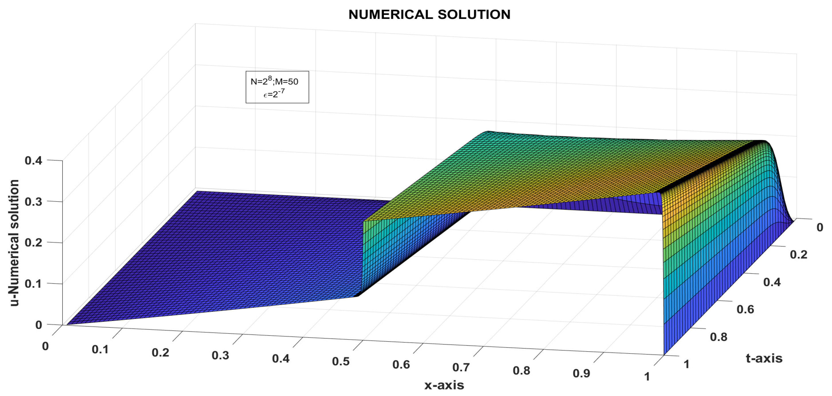
Figure 1. Numerical solution of Example 1.
Mathematics 11 02034 g001
Figure 2. Maximum error of Example 1, when M = 50 .
Mathematics 11 02034 g002
Figure 3. Numerical solution of Example 2.
Mathematics 11 02034 g003
Figure 4. Maximum error of Example 2, when M = 50 .
Mathematics 11 02034 g004
Table 1. Maximum error and order of convergence for Example 1 with the number M = 50,100.
ε MN (Number of Grid Points)
2 6 2 7 2 8 2 9 2 10 2 11 2 12
2 6 501.0843 × 10 1 3.1740 × 10 2 1.2410 × 10 2 4.0043 × 10 3 1.2979 × 10 3 3.6024 × 10 4 1.0865 × 10 4
1001.0286 × 10 1 2.6681 × 10 2 1.0315 × 10 2 3.7978 × 10 3 1.5062 × 10 3 6.2557 × 10 4 2.6478 × 10 4
2 7 501.1120 × 10 1 2.8842 × 10 2 1.1237 × 10 2 3.5721 × 10 3 1.1214 × 10 3 3.9296 × 10 4 1.6141 × 10 4
1001.0748 × 10 1 2.8066 × 10 2 1.1374 × 10 2 4.6676 × 10 3 1.8575 × 10 3 8.9909 × 10 4 4.2970 × 10 4
2 8 501.1289 × 10 1 2.7113 × 10 2 1.0495 × 10 2 3.2872 × 10 3 1.2105 × 10 3 4.5429 × 10 4 1.9634 × 10 4
1001.1002 × 10 1 2.9689 × 10 2 1.2033 × 10 2 5.0398 × 10 3 2.4171 × 10 3 1.1748 × 10 3 5.8837 × 10 4
2 9 501.1361 × 10 1 2.6175 × 10 2 1.0085 × 10 2 3.2652 × 10 3 1.2404 × 10 3 5.0069 × 10 4 2.1944 × 10 4
1001.1175 × 10 1 3.0602 × 10 2 1.2410 × 10 2 5.3361 × 10 3 2.5656 × 10 3 1.3340 × 10 3 6.5985 × 10 4
2 10 501.1395 × 10 1 2.5686 × 10 2 9.8700 × 10 3 3.3070 × 10 3 1.2620 × 10 3 5.1495 × 10 4 2.3576 × 10 4
1001.1263 × 10 1 3.1082 × 10 2 1.2609 × 10 2 5.5213 × 10 3 2.6932 × 10 3 1.3756 × 10 3 7.0938 × 10 4
2 11 501.1411 × 10 1 2.5438 × 10 2 9.7602 × 10 3 3.3285 × 10 3 1.2731 × 10 3 5.2436 × 10 4 2.4101 × 10 4
1001.1307 × 10 1 3.1327 × 10 2 1.2711 × 10 2 5.6167 × 10 3 2.7588 × 10 3 1.4141 × 10 3 7.2555 × 10 4
2 12 501.1418 × 10 1 2.5312 × 10 2 9.7046 × 10 3 3.3393 × 10 3 1.2787 × 10 3 5.2911 × 10 4 2.4429 × 10 4
1001.1329 × 10 1 3.1451 × 10 2 1.2763 × 10 2 5.6650 × 10 3 2.7921 × 10 3 1.4321 × 10 3 7.3508 × 10 4
2 13 501.1422 × 10 1 2.5249 × 10 2 9.6767 × 10 3 3.3448 × 10 3 1.2815 × 10 3 5.3150 × 10 4 2.4594 × 10 4
1001.1340 × 10 1 3.1514 × 10 2 1.2789 × 10 2 5.6894 × 10 3 2.8088 × 10 3 1.4416 × 10 3 7.3966 × 10 4
2 14 501.1424 × 10 1 2.5217 × 10 2 9.6627 × 10 3 3.3475 × 10 3 1.2829 × 10 3 5.3270 × 10 4 2.4679 × 10 4
1001.1345 × 10 1 3.1545 × 10 2 1.2803 × 10 2 5.7016 × 10 3 2.8172 × 10 3 1.4469 × 10 3 7.4190 × 10 4
2 15 501.1425 × 10 1 2.5201 × 10 2 9.6557 × 10 3 3.3489 × 10 3 1.2836 × 10 3 5.3330 × 10 4 2.4725 × 10 4
1001.1348 × 10 1 3.1561 × 10 2 1.2809 × 10 2 5.7077 × 10 3 2.8214 × 10 3 1.4496 × 10 3 7.4301 × 10 4
D x N , k 501.1425 × 10 1 3.1740 × 10 2 1.2410 × 10 2 4.0043 × 10 3 1.2979 × 10 3 5.3330 × 10 4 2.4725 × 10 4
1001.1348 × 10 1 3.1561 × 10 2 1.2809 × 10 2 5.7077 × 10 3 2.8214 × 10 3 1.4496 × 10 3 7.4301 × 10 4
r N , k 501.8478 × 10 0 1.3548 × 10 0 1.6319 × 10 0 1.6253 × 10 0 1.2832 × 10 0 1.1089 × 10 0 -
1001.8462 × 10 0 1.3010 × 10 0 1.1662 × 10 0 1.0165 × 10 0 9.6076 × 10 1 9.6419 × 10 1 -
Table 2. Maximum error and order of convergence for Example 2 with the number M = 50,100.
ε MN (Number of Grid Points)
2 6 2 7 2 8 2 9 2 10 2 11 2 12
2 6 502.1266 × 10 1 1.3349 × 10 1 7.0424 × 10 2 3.3712 × 10 2 1.5223 × 10 2 7.1724 × 10 3 3.4900 × 10 3
1002.8109 × 10 1 2.2380 × 10 1 1.3696 × 10 1 7.0987 × 10 2 3.3312 × 10 2 1.5960 × 10 2 7.8452 × 10 3
2 7 503.5020 × 10 1 2.2511 × 10 1 1.2890 × 10 1 6.7146 × 10 2 3.3507 × 10 2 1.6344 × 10 2 7.8856 × 10 3
1004.5196 × 10 1 3.8586 × 10 1 2.6099 × 10 1 1.4770 × 10 1 7.6575 × 10 2 3.8040 × 10 2 1.8516 × 10 2
2 8 504.4469 × 10 1 3.0061 × 10 1 1.7211 × 10 1 9.0480 × 10 2 4.6009 × 10 2 2.3068 × 10 2 1.1432 × 10 2
1005.8200 × 10 1 5.2658 × 10 1 3.6716 × 10 1 2.1077 × 10 1 1.1126 × 10 1 5.6420 × 10 2 2.8120 × 10 2
2 9 505.0400 × 10 1 3.4278 × 10 1 1.9902 × 10 1 1.0568 × 10 1 5.3720 × 10 2 2.7130 × 10 2 1.3529 × 10 2
1006.6504 × 10 1 6.0947 × 10 1 4.3599 × 10 1 2.5668 × 10 1 1.3564 × 10 1 6.9369 × 10 2 3.4832 × 10 2
2 10 505.3763 × 10 1 3.6934 × 10 1 2.1445 × 10 1 1.1366 × 10 1 5.8382 × 10 2 2.9379 × 10 2 1.4749 × 10 2
1007.1658 × 10 1 6.5915 × 10 1 4.7996 × 10 1 2.8410 × 10 1 1.5157 × 10 1 7.7503 × 10 2 3.8981 × 10 2
2 11 505.5558 × 10 1 3.8344 × 10 1 2.2246 × 10 1 1.1819 × 10 1 6.0637 × 10 2 3.0661 × 10 2 1.5383 × 10 2
1007.4477 × 10 1 6.8558 × 10 1 5.0407 × 10 1 3.0050 × 10 1 1.6044 × 10 1 8.2210 × 10 2 4.1429 × 10 2
2 12 505.6486 × 10 1 3.9071 × 10 1 2.2677 × 10 1 1.2054 × 10 1 6.1870 × 10 2 3.1290 × 10 2 1.5730 × 10 2
1007.6104 × 10 1 6.9976 × 10 1 5.1666 × 10 1 3.0910 × 10 1 1.6535 × 10 1 8.4716 × 10 2 4.2767 × 10 2
2 13 505.6958 × 10 1 3.9441 × 10 1 2.2904 × 10 1 1.2175 × 10 1 6.2500 × 10 2 3.1619 × 10 2 1.5897 × 10 2
1007.6927 × 10 1 7.0691 × 10 1 5.2310 × 10 1 3.1350 × 10 1 1.6788 × 10 1 8.6049 × 10 2 4.3442 × 10 2
2 14 505.7196 × 10 1 3.9627 × 10 1 2.3017 × 10 1 1.2236 × 10 1 6.2816 × 10 2 3.1785 × 10 2 1.5984 × 10 2
1007.7341 × 10 1 7.1050 × 10 1 5.2636 × 10 1 3.1573 × 10 1 1.6915 × 10 1 8.6729 × 10 2 4.3793 × 10 2
2 15 505.7315 × 10 1 3.9720 × 10 1 2.3074 × 10 1 1.2267 × 10 1 6.2975 × 10 2 3.1868 × 10 2 1.6027 × 10 2
1007.7548 × 10 1 7.1230 × 10 1 5.2803 × 10 1 3.1685 × 10 1 1.6980 × 10 1 8.7074 × 10 2 4.3971 × 10 2
D x N , k 505.7315 × 10 1 3.9720 × 10 1 2.3074 × 10 1 1.2267 × 10 1 6.2975 × 10 2 3.1868 × 10 2 1.6027 × 10 2
1007.7548 × 10 1 7.1230 × 10 1 5.2803 × 10 1 3.1685 × 10 1 1.6980 × 10 1 8.7074 × 10 2 4.3971 × 10 2
r N , k 505.2904 × 10 1 7.8358 × 10 1 9.1156 × 10 1 9.6189 × 10 1 9.8265 × 10 1 9.9160 × 10 1 -
1001.2260 × 10 1 4.3187 × 10 1 7.3683 × 10 1 8.9999 × 10 1 9.6349 × 10 1 9.8568 × 10 1 -
Disclaimer/Publisher’s Note: The statements, opinions and data contained in all publications are solely those of the individual author(s) and contributor(s) and not of MDPI and/or the editor(s). MDPI and/or the editor(s) disclaim responsibility for any injury to people or property resulting from any ideas, methods, instructions or products referred to in the content.