1. Introduction
A certain water lift station, receiving a continuous but variable and unknown flow of water, is equipped with three water pumps to release water and thus prevent the overflow of the tank. Activation and deactivation of the pumps depends on the water level (measured in meters), according to predefined thresholds, as given in
Table 1 and explained next. The tank is also equipped with sensors that read, at 5 min intervals, the water level and the number of active pumps. In order to better understand the scope of our objectives, a small sample of the database, which spans an entire year, is displayed in
Table 2.
We shall denote the thresholds , and using , and , respectively, and the thresholds , and using , and , respectively. We will refer to , and as the upward thresholds and to , and as the downward thresholds. We denote, using , the number of active pumps at time step n and refer to it as the status of the system at time n.
The system operates according to the following rules. In case no pump is active and an increasing water level reaches , the first pump is activated. Similarly, in case only one pump is (or, respectively, two pumps are) active and the water level reaches (or, respectively, ), a second (or, respectively, third) pump is activated. Analogously, in case all three pumps are working and the water level drops below , one pump is deactivated; if the level keeps lowering and reaches , another pump stops working, and if the level reaches the level , the remaining active pump is switched off. In other words:
When none of the pumps is working, the status of the system will not change unless the water level reaches ;
When only one pump is working, the status of the system will not change unless the water level reaches or drops below ;
When two pumps are working, the status of the system will not change unless the water level reaches or drops below ;
When all three pumps are working, the status of the system will not change unless the water level drops below .
Figure 1 shows, for 60 consecutive entries of the database (the first 20 of which constitute the data given in
Table 2), the water level and the corresponding number of active pumps as given in the data set.
Whereas the data relative to the water level can be considered accurate (apart from occasional typos, such as negative values and values significantly below
or above
), the data relative to the number of active pumps is easily seen to contain errors. For example, in Reading 3 from
Table 2, the correct number of active pumps must be at least 2, since the water level had already reached
, prompting a second pump to switch on (for a better visualization, we refer to Reading 4 on
Figure 1, where the threshold
is clearly attained). Another example is Reading 14, where the level
was already reached, so the number of active pumps is 3, and it should only decrease to 2 at Reading 16, when
is reached. Whenever detected, these values are replaced with one consistent with the remaining data, and we will make a thorough description in
Section 2 of the criteria to determine the correct value at each time step.
In order to estimate for how long the pumps have been working, we model the level of the water continuously, so that we may estimate at which instant a pump has been activated or deactivated. To do so, we first identify under which conditions one or more thresholds have been attained in the interval of time under analysis, according to the data for the near past and near future of the interval. We then design an algorithm that models the water level, taking into account the switching on and off of the pumps, as well as an associated delay.
Given that both the data and common sense suggest that the effect of a pump being activated or deactivated may not be immediate and that the influx of water is variable and unknown, we consider a minimum delay of 5 s and a maximum delay of 15 s. Although empirical, these values are sustained by the data. For example, there exist readings above an upward threshold which are followed by a decrease in water level, meaning that the water level did not start to decrease immediately after the threshold was attained. Further evidence of this fact is the existence of values below and above . Thus, let and (measured in time steps). Delays within and are called admissible.
Concerning the literature on this framework, several recent works used machine learning tools to address problems, and goals, similar to ours. For example, in [
1], the authors take an approach to fill gaps on a scarce data time series using the MissForest algorithm, and, in [
2], gap filling is achieved by means of automated evolutionary identification of the optimal structure for a composite data-driven model. Our data set, however, contains a large number of errors in the status time series and thus does not provide a reliable training set for the application of machine learning regression techniques to infer the status of the system. Therefore, even though the status inference (with errors) from the water-level time series has an accuracy of
by means of the application of a random forest algorithm (cf. the public GitHub repository indicated at the end of this work), this will not allow for acquisition of the real status values, since it accurately predicts the status with those errors.
In [
3], a multiple-point statistics algorithm suited for pattern reproduction is used. The main advantage of this method is its ability to provide probabilistic estimates of the missing values, which allows for uncertainty quantification. Although uncertainty is obviously also present in our problem, in our framework, pattern recognition benefits greatly from taking into account contextualized hands-on information about the system. For this reason, we favored an approach of a more deterministic nature, where uncertainty is addressed by providing criteria that establish which status change is most likely to have happened. The subsequent data gaps are then filled by means of several synchronized steps of linear interpolation.
A different, but related, possible approach to status inference would be an error-correction method, similar to those studied in [
4] in an econometrics environment. Our framework is not related, since the corrections that we are interested in are based on empirical information and not on any difficulty in finding a fit model that performs the regression between the two time series.
Regarding data completion, we note that, in our problem, the gaps are the time values between the 5 min time steps instead of the erratic and larger gaps often considered in the literature. Several regression methods for gap filling between regular time steps can be found easily in the literature. For example, in [
5], the author gives some insight on how to fit a discrete data time series into a continuous time function. Again, in our framework, the complexity arises from information outside the data set (threshold crossing and delays) and not with any difficulty in finding an appropriate regression model in particular. Other methods range from simple linear models to complex deterministic or stochastic techniques. Common approaches include, for example, the simple nearest neighbor method via data transfer [
6], interpolation techniques [
7], auto-regressive models [
8], and simple and multiple regressions [
9].
In short, to accomplish our goal, we first design an algorithm to predict the system status. Based on the previous and next water level readings of a given time step, this procedure identifies the thresholds, if any, that have been crossed between this and the following time step. Next, we define rules to model the water level, filling the gaps between the 5 min time steps continuously with piecewise linear functions. These rules follow these required principles:
Take the water level readings from the original data set as constraints, since these are considered to be correct;
Have the water level behave according to every previously identified change of status;
Take into consideration the fact that the effect of the activation and deactivation of a pump on water level is not immediate, but rather comes with a certain delay.
Combining the status inference—that is, the estimated number of active pumps at each reading—with the estimated water level, we are able to determine the moment when each pump has been activated or deactivated. This allows for fulfillment of the company’s ultimate objective, which is to estimate for how long each pump has been active.
This paper is organized in the following way: in the next section, we determine the conditions under which the status of the system changes; in the following section, we define how the gaps between readings should be filled for each type of transition; the fourth section is devoted to the implementation of
Section 2 and
Section 3 on a sample of the data set; and in the final section, we present an analysis of the results obtained.
2. Inferring the System Status
As stated before, we consider the water-level time series to be accurate, and so any incoherence between the water-level readings and the number of active pumps is due to an error in the latter.
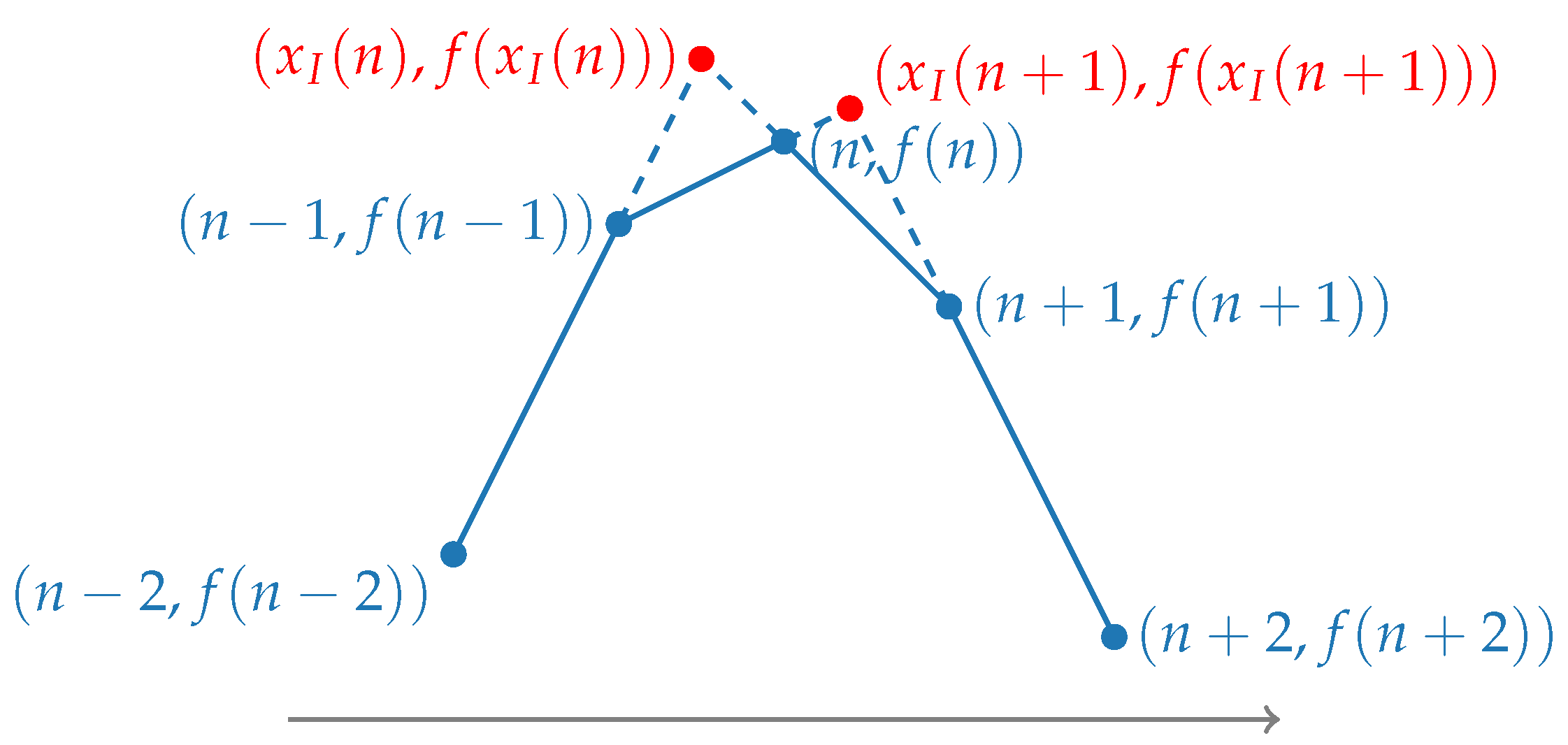
In this section we will describe a detailed procedure to obtain the correct status of the system at every time step n, and to do this we must consider what happens both before and after n. Moreover, the conclusions will be obtained using not only the water-level readings, but also the rate changes, in order to encompass the trend of the water level. The procedure not only addresses the reasons to infer changes in the status, but it also establishes prioritization criteria that allows us to settle which changes are the most likely to have occurred.
Let
denote the rate corresponding to the difference between the water level at time step
n and
. If the line that contains
and
and the line that contains
and
intersect within
, we denote the
x-coordinate of this point using
.
Figure 2 exemplifies the existence and non-existence of
.
An analysis of the data set allows us to infer some useful properties of the system, namely:
for the whole data set;
for the whole data set;
If , then (this means that whenever all the pumps are simultaneously active, the water level decreases);
If , then (this means that the minimum inflow of water into the system is of m per 5 min). As a consequence, since , the system is never fully turned off for more than three time steps;
If and , then some threshold must have been crossed within —if not within nor , then within ;
If , and , then the upward threshold was crossed;
Similarly, if , and , then the downward threshold was crossed;
If or , then the corresponding threshold was crossed.
Next, we establish the conditions under which the system status changes from a time step
to a time step
n. For simplicity and ease of reference, these conditions are listed in
Table 3,
Table 4,
Table 5 and
Table 6.
The main challenge is, of course, to identify which conditions imply that a certain status change takes place. Based on the analysis above, we consider four distinct conditions as evidence of a change from a status k to a neighbouring status and three distinct conditions as evidence of a change from a status k to a non-neighbouring status with . Moreover, due to the fact that the transition from a status k to a status and the transition from a status to a status , both being transitions between neighbouring statuses, share similarities between them, the four conditions are precisely of the same type in both cases. The same applies to transitions between non-neighbouring statuses. Thus, overall, will be different than if one of the following occurs:
- (a)
An explicit crossing of the relevant threshold;
- (b)
Evidence of the trend before and the trend after n meeting at a water level higher/lower than or close enough to the relevant threshold within more likely than later on;
- (c)
For changes between neighbouring statuses, evidence of a sharp change from a positive/negative to a negative/positive ;
- (d)
Evidence of a significant change from a positive/negative to a negative/positive coexisting in a reading close to the relevant threshold.
We shall detail the transition of to , with the remaining transitions following analogous reasoning. As shorthand to make our arguments more concise, in the remainder of this work, both the conditions and will always be considered satisfied if exists and does not exist.
For
to go from 2 to 3 between
and
n, the water level must have reached the upward threshold
during this interval. This is obviously the case if the water level is at least
at
n, that is, if
. Since this is a condition of type “a”, we shall denote it with (23a). Of course, it may also happen that, although
was attained during the interval
, the water level is no longer above
by the time reading
n takes place. One evidence of this fact is that the trend before
and the trend after
n meet at a water level higher than or close enough to
within
, that is,
, along with an extra condition,
, which ensures that the change is more likely to have happened in
than later on. Since this condition is of type “b”, we labeled it (23b). Given that 2 and 3 are neighbouring statuses, a sharp change from a positive
to a negative
is also indicative of the water level having attained
during
. Thus, having
and
, along with the same extra condition,
, which was included in (23b), is evidence of a status change from 2 to 3, and will be labeled (23c).
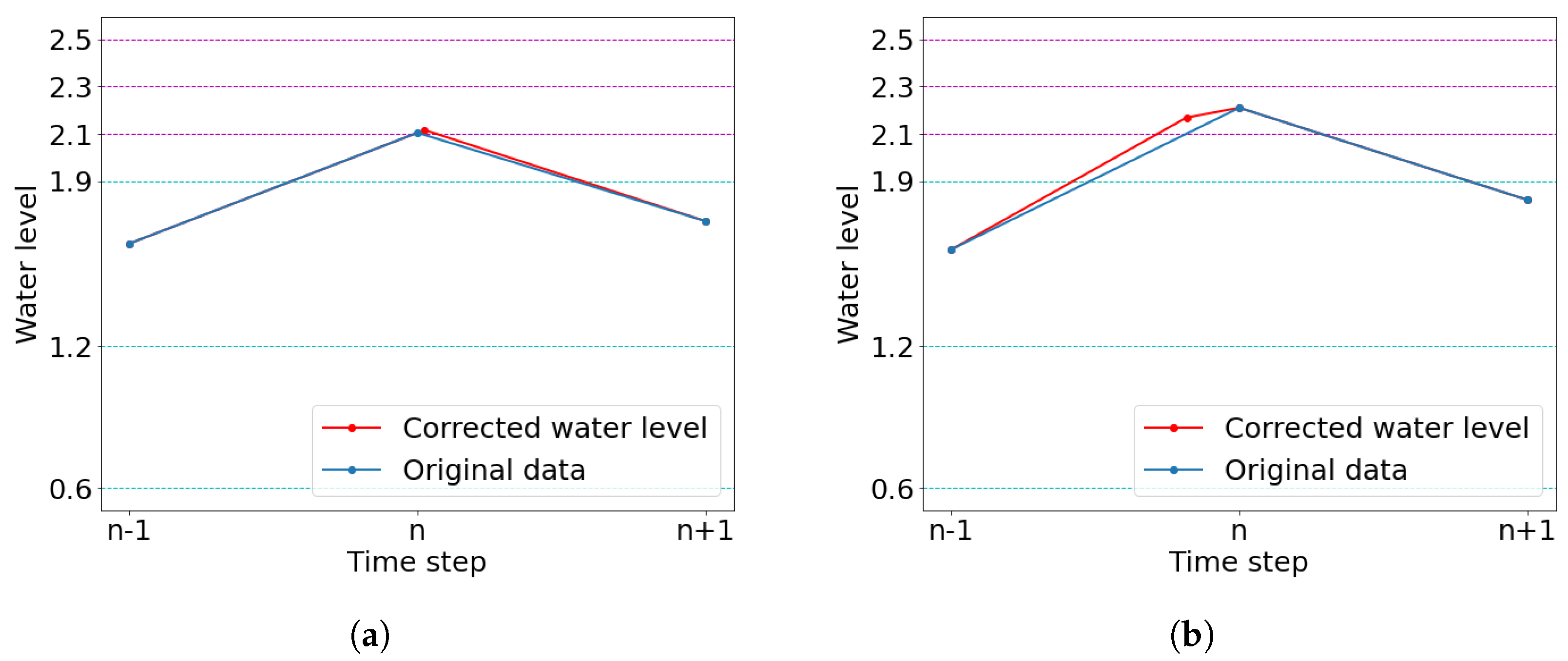
Figure 3 illustrates conditions (23b) and (23c), according to whether
sits below or above
, respectively. Finally, if a significant change from a positive
to a negative
coexists in a reading close to
, quantified as
,
, we also consider that the status changed from 2 to 3. This condition is labeled (23d). If none of the conditions (23a), (23b), (23c) or (23d) is met, we conclude that the status remains unchanged.
It is also important to note that the order in which these conditions should be verified, given a status , is not entirely random. To prevent the change from being underestimated, the status farthest possible from k must be checked first, the status second farthest from k must be checked next, and so on (but it makes no difference whether one first checks if or ).
3. Data Gap Completion
Having established that the status of the system will change from a time step to a time step n—along with exactly which change will take place and the reason such a change will occur, that is, the type of condition (“a”, “b”, “c” or “d”) that applies—we aim to continuously describe the water level, completing the information that the system does not convey regarding the water level. In this section, we establish how this completion should be accomplished for each of the status transition conditions identified in the previous section. We detail the procedure to follow for crossing the upward thresholds, since crossing the downward thresholds has entirely symmetrical consequences on the water level. Recall that we always allow for a delay, between and , from the instant when a pump is activated or deactivated to the instant when its effect on the water level takes place.
To ease the notation, the water level at time step n will be denoted as instead of , and the rate will be denoted as . If the line segment that joins and intersects or, in case this intersection does not exist, if the line segment that joins and intersects , we denote this point as .
In case there is no change of status between readings and n, the water level is given by the linear function that joins and . The task is thus to establish how to fill the gaps when it has been determined that the status changed between two consecutive readings. The procedure must ensure that the relevant threshold(s) was(were) indeed crossed, verify the existence of a delay within the given limits, and verify a change in the rate of the water level once this delay is fulfilled. This is accomplished with a piecewise linear function, with the smallest possible difference from the linear function connecting the readings.
The procedure also takes into account the type of condition that sustains the status change. In fact, if the condition is of type “a”, we have a reading above/below the relevant threshold, so that it is guaranteed that the water level will cross the threshold (and the adjustments to make, if any, have to do with ensuring an admissible delay), whereas in a condition of type “b”, this crossing must be accomplished between
and
n. Likewise, conditions of type “c” and “d” have their own specificity. On the other hand, the procedure functions differently accordingly to the number of thresholds crossed. Therefore, we consider the following cases (recall that conditions of type “c” only exist for transitions between neighbouring statuses):
| A1/A2/A3: | for transitions of type “a” in which 1/2/3 thresholds are crossed; |
| B1/B2/B3: | for transitions of type “b” in which 1/2/3 thresholds are crossed; |
| C1: | for transitions of type “c”; |
| D1/D2/D3: | for transitions of type “d” in which 1/2/3 thresholds are crossed. |
The remainder of this section is devoted to describing the procedure followed in each of these cases.
3.1. Case A1: Transitions of Type (01a), (12a) and (23a)
In this case, is given by the intersection of a line segment that joins and with . Notice that represents the delay by which the water level is affected following the crossing of (and consequent activation of the pump). There are three sub-cases to consider:
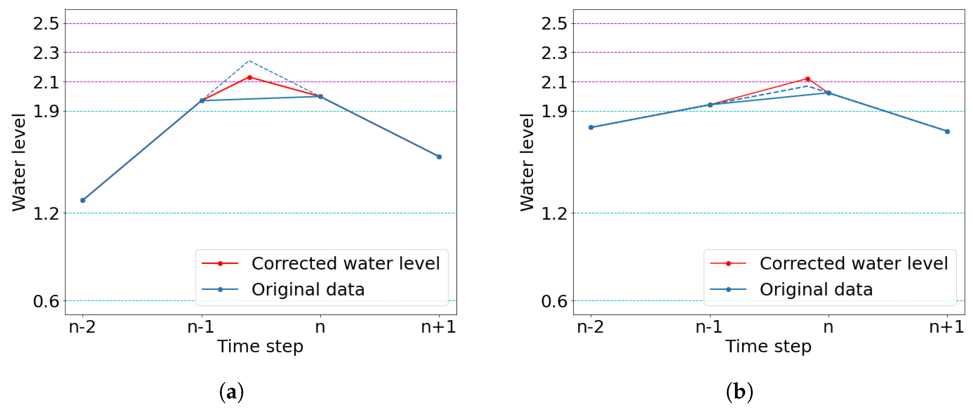
A1 (i). A1 (ii). A1 (iii). .
Case A1 (i) requires no intervention, since the delay is within the admissible values. If A1 (ii) occurs, we shift the maximum towards the right, along the line segment that joins
and
, in order to comply with the minimum delay, that is, a delay of
. Notice that the water level at the new maximum will not exceed
. In fact, since the maximum is attained at
, for the water level to reach the next threshold, we would have
which is impossible in this framework. Finally, in case A1 (iii), we split the the line segment that joins
and
into two line segments. If
and
, the break point will be at
along the line that contains
and
—since
sits
to the left of
, we thus ensure a delay of
; since
, the water level at
will be at most
, and so
is not reached. If
or
, the first line segment leaves
with a slope of
and halts at
—again, the delay of
is ensured, and, since
in this framework,
is guaranteed as well. In either case, the second line segment is the one that joins the break point and
.
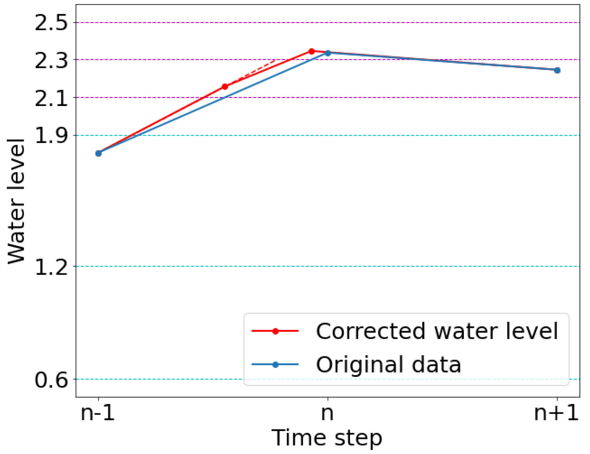
Figure 4 illustrates sub-cases A1 (ii) and A1 (iii). The blue dots represent actual data entries (and blue line segments represent the water level as given directly by the readings), and the red dots represent additional break points, as given by the rules adopted (and red line segments represent the corrected water level). The purple (respectively, light blue) dashed lines help to locate the upward (respectively, downward) thresholds. This color code will be adopted throughout the entire work.
3.2. Case B1: Transitions of Type (01b), (12b) and (23b)
This turn, is given by the intersection of a line segment that joins and with . We consider the following sub-cases:
B1 (i):
B1 (ii):
B1 (iii):
B1 (iv): .
Again, case B1 (i) requires no correction. In case B1 (ii), we proceed as in case A1 (ii), using
instead of
. In case B1 (iii), we lower
to
, so that the line segment that joins
and
intersects
in such a way that the delay equals
. To be precise, we have
Finally, in case B1 (iv), we proceed symmetrically to case B1 (iii), shifting the point
upwards to
, but this turn occurs in order to get a delay of
, namely,
Figure 5 illustrates sub-cases of (iii) and (iv) of case B1. The dotted line segments indicate the extension of the previous or future line segments, and so
is their intersection point.
3.3. Case C1: Transitions of Type (01c), (12c) and (23c)
In the case when exists, but case B1 does not apply (and so ) and the evidence of a threshold crossing comes from the sharp change from to (in this case, from a positive to a negative ) along with (or the non-existence of ), we nonetheless proceed as in case B1 (iv).
3.4. Case D1: Transitions of Type (01d), (12d) and (23d)
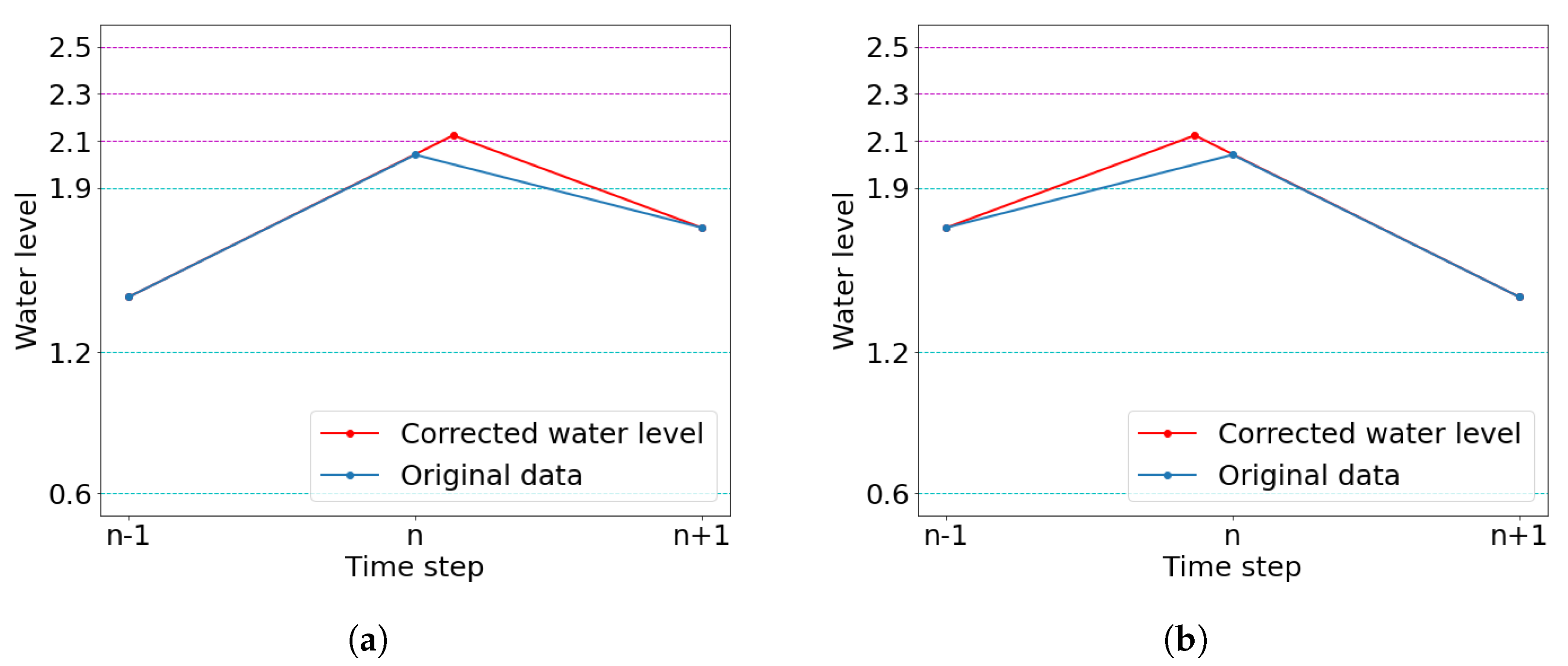
This turn, the evidence of a threshold crossing is given by a reading close to a threshold together with a significant change and opposite signs in
to
. We proceed similarly in the two sub-cases
considering we extend the line segment with the greatest incline, allowing for a minimum delay.
Figure 6 illustrates the sub-cases of (i) and (ii) of case D1, respectively.
3.5. Case A2: Transitions of Type (02a) and (13a)
In this case, one or two additional break points are defined, following the same principles that were adopted in case A1. Given that the uncorrected version yields an exaggerated delay after the first threshold has been reached, we first proceed as in case A1 (iii). Therefore, we split the line segment between
and
into two line segments, with a break point sitting
to the left of the point where the line segment that joins
and
meets the first threshold. Next, we consider the line segment that joins the first break point and
and again apply the appropriate the sub-case of A1.
Figure 7 illustrates an instance of case A2.
3.6. Case B2: Transitions of Type (02b) and (13b)
As in case B1,
is given by the intersection of a line segment that joins
and
with
. We set a first break point at
along the line that contains
and
. In case the line segment that joins the first break point and
yields an admissible delay when crossing the second threshold, we take
to be the local maximum; otherwise, we proceed as in cases B1 (ii), (iii) or (iv), adjusting the maximum value
in order of the corresponding delay to be within the interval
.
Figure 8 illustrates case B2.
3.7. Case D2: Transitions of Type (02d) and (13d)
Here, we determine a first break point using the procedure established for case A1 (iii) and then apply the appropriate sub-case of case D1, according to whose line segment has the greatest incline: the line segment joining the first break point and or the line segment joining and .
3.8. Case A3: Transitions of Type (03a)
This case is dealt with analogously to case A2, now with the introduction of an extra initial break point. In order to obtain a more natural decay in the rate of the water level, we consider that the water level reaches at (thus anticipating the crossing of the first threshold) and that the first break point occurs at .
3.9. Case B3: Transitions of Type (03b)
Analogous to case A3, we introduce the extra initial break point, as defined there, and then proceed as in case B2.
3.10. Case D3: Transitions of Type (03d)
Again, we introduce the extra initial break point and then proceed as in case D2.
4. Implementation on a Sample of the Data Set
In this section, we apply the algorithms from
Section 2 and
Section 3 to a sample of the data set and analyse the results obtained. For purposes of this exercise, and since the initial reading is
, we consider that the status for the first reading, as given in the data set, is correct. Thus,
.
We begin by inferring the status of the system as described in
Table 3,
Table 4,
Table 5 and
Table 6. The status change condition, if any, that applies to each row of the sample displayed in
Table 2, together with the corrected status of the system, is indicated in
Table 7.
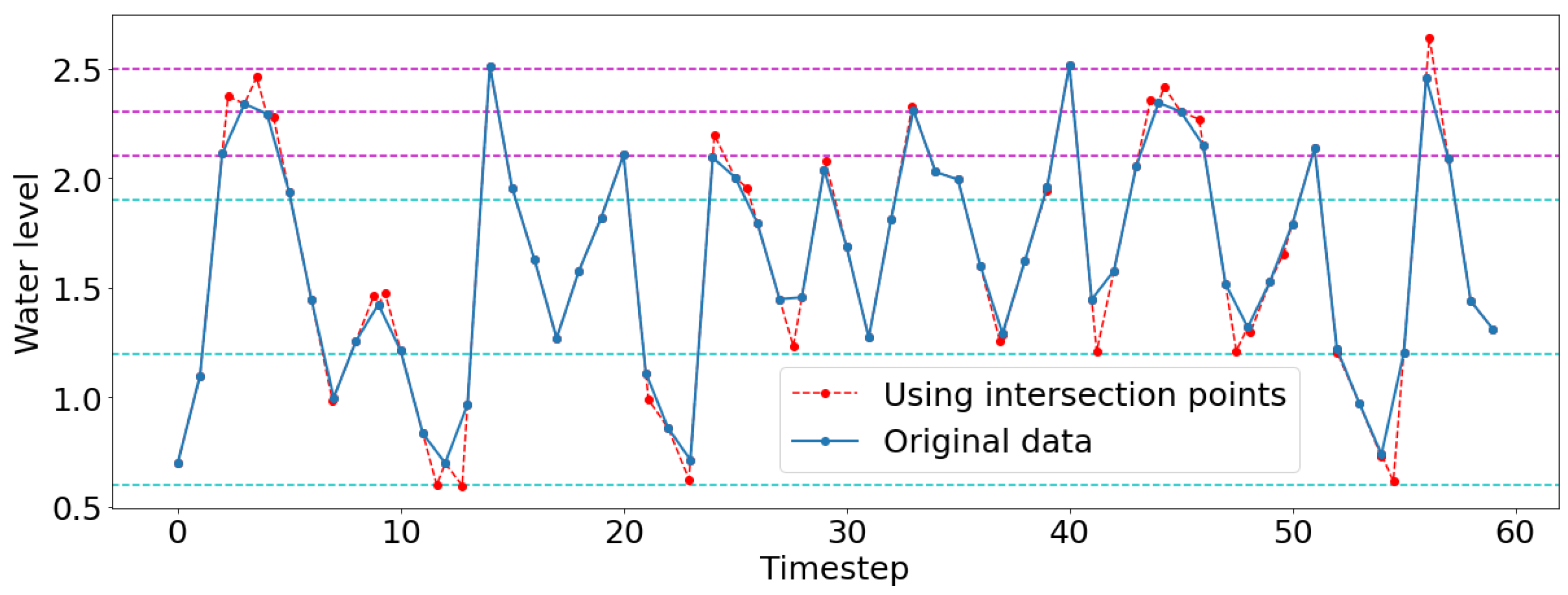
Figure 9 shows the water level as given by the data along with the points
, when they exist. As we saw in
Section 2, these points are instrumental when deciding the status transitions.
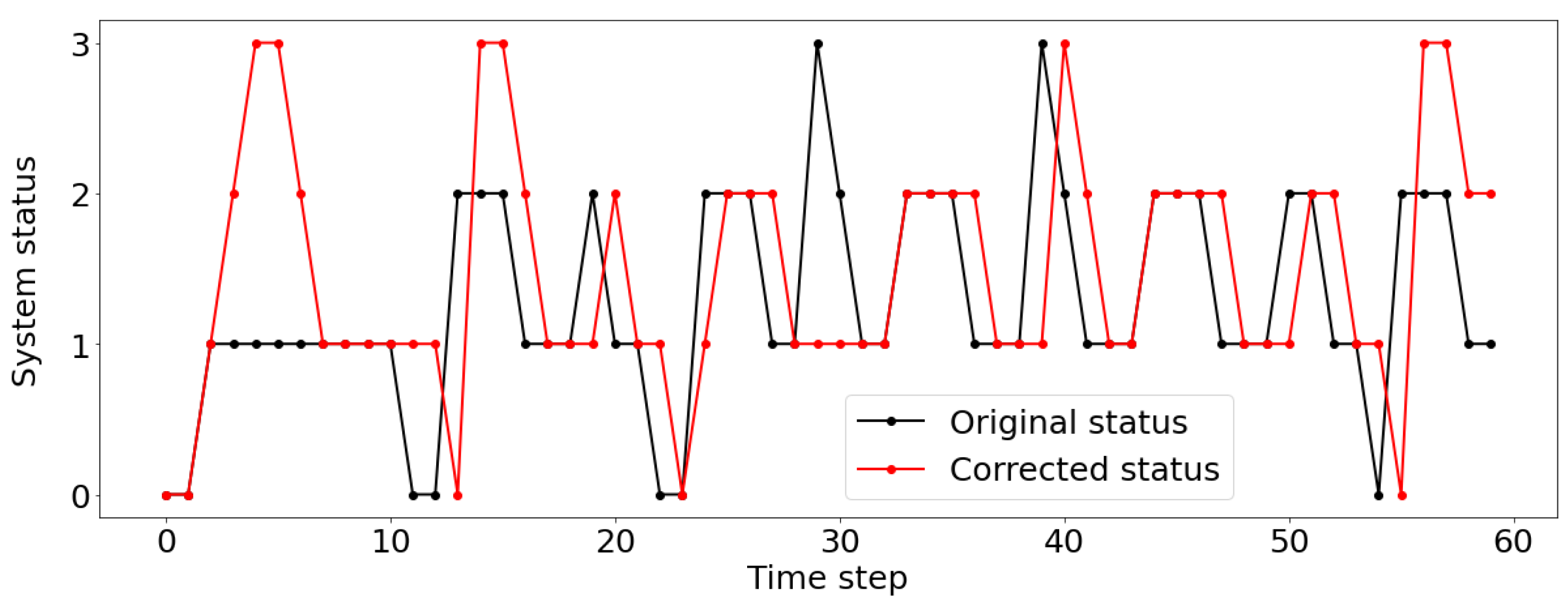
Figure 10 exhibits the comparison between the system status given in the data set and the corrected status at each time step (in black, as given by the data set, and in red, as given by the status inference set up in
Section 2). Overall, this sample of the original data set yields a total of 78 5-min “active intervals”, that is, 5-min intervals (some of which coincide in time) during which a pump was active, whereas the corrected version yields a total of 89 such intervals.
For comparison, we remark that, in the original (complete) data set, there were 7971 5-min intervals in which no pump was working, 53,107 5-min intervals in which one pump was working, 8924 5-min intervals in which two pumps were working and 41 5-min intervals in which all pumps were working. Applying the status inference algorithm to the whole data set, these figures become 9251, 39,531, 18,120 and 3141, respectively. It is particularly striking how the full operation of the pumps was being underestimated.
Detailing individually for each of the three pumps, the correction of the status determined by
Section 2 yields a total of 30 5-min active intervals for pump 1, 21 5-min active intervals for pump 2 and 38 5-min active intervals for pump 3. (This analysis, impossible to perform on the original data on account of its incoherence, uses the
modus operandi of the system: when activating a pump, the system chooses the one that has been switched off longest and similarly for deactivation.)
Taking into account the modeling of the water level set up in
Section 3, which always anticipates or delays the change of status, these values become
,
and
, respectively. Thus, comparing the un-modeled with the modeled version, pump 1 works approximately
less of the time, pump 2 works approximately
less of the time, pump 3 works roughly the same time, and the system works approximately
less of the time (the total having become
5-min units).
Figure 11 displays the comparison between the moment when each pump is activated and deactivated (in black, as given by the status inference algorithm from
Section 2, and in red, as given by the modeling established in
Section 3).
Finally,
Figure 12 displays the water level as given by the original data (blue dashed line) and the water level as modeled in
Section 3 (red continuous line). For a better visualization, we focus on the first 20 entries of the sample under analysis. These graphs show how the gap completion preserves the water level readings and the extra break points introduced by this algorithm, with the consequent anticipation/retardation of the crossing of the thresholds when compared with the original data. The crossing of every appropriate threshold(s) and the delayed effect of the activation and deactivation of the pumps after each threshold crossing on the water level can also be observed. The outcome is that the response of the system is always coherent with its operating mode.


