A Novel Fractional-Order RothC Model

Abstract

A new fractional q-order variation of the RothC model for the dynamics of soil organic carbon is introduced. A computational method based on the discretization of the analytic solution along with the finite-difference technique are suggested and the stability results for the latter are given. The accuracy of the scheme, in terms of the temporal step size h, is confirmed through numerical testing of a constructed analytic solution. The effectiveness of the proposed discrete method is compared with that of the classical discrete RothC model. Results from real-world experiments show that, by adjusting the fractional order q and the multiplier term $\zeta (t,q)$, a better match between simulated and actual data can be achieved compared to the traditional integer-order model.

1. Introduction

Soil carbon dynamics models describe the processes that govern the exchange of carbon between the soil and the atmosphere. They help in understanding the role of soils in the global carbon cycle and the impact of land use and management practices on soil carbon stocks [1]. One of the most widely used models in this field is the Rothamsted Carbon Model [2,3] (RothC), which is a process-based model that simulates soil organic matter dynamics in response to changes in land use and management. RothC considers a number of important factors, including the decomposition of organic matter, changes in soil moisture and temperature, and the effect of ploughing or other agricultural practices on soil carbon capture and storage. By providing a comprehensive representation of soil carbon dynamics, RothC has become a valuable tool in evaluating the impact of land use and management strategies on soil carbon sequestration and in making predictions about trends in soil carbon stocks under the effect of rising temperatures due to global climate change [4,5].

The RothC model analyzes the dynamics of soil carbon by splitting it into five compartments, four active with different chemical degradation characteristics, and one inactive that is resistant to decomposition. The original monthly time-stepping procedure was recently improved by the non-standard approaches proposed in [6]. As in real soil systems, the processes are continuous in time; the following formulation of the RothC model was given in [7]:

$${\displaystyle \frac{d\mathbf{c}}{dt}=\rho \left(t\right)A\mathbf{c}+\mathbf{b}\left(t\right)}$$

(1)

where $\mathbf{c}\left(t\right)={[c_{dpm}\left(t\right),c_{rpm}\left(t\right),c_{bio}\left(t\right),c_{hum}\left(t\right)]}^T$ indicates the concentration of different compartments: decomposable plant material (DPM), resistant plant material (RPM), microbial biomass (BIO) and humified organic matter (HUM). The rate modifier $\rho \left(t\right)$ depends on land cover, soil, and climatic variables. The model (1) is given in terms of the matrix A, defined as

$$A=\left(\begin{array}{cccc}-k_{dpm}& 0& 0& 0\\ 0& -k_{rpm}& 0& 0\\ \alpha k_{dpm}& \alpha k_{rpm}& (\alpha -1)k_{bio}& \alpha k_{hum}\\ \beta k_{dpm}& \beta k_{rpm}& \beta k_{bio}& (\beta -1)k_{hum}\end{array}\right).$$

where $\mathbf{k}=[k_{dpm},k_{rpm},k_{bio},k_{hum}]$ are the decomposition rate constants, while $\alpha$ and $\beta$ represent the fractions of metabolized carbon incorporated into the compartments $c_{bio}\left(t\right)$ and $c_{hum}\left(t\right)$; the remaining part $1-\alpha -\beta$ is the fraction of metabolized carbon lost by the system in the form of $C{O}_2$.

At time t, the carbon level entering the system is represented by the vector

$$\mathbf{b}\left(t\right):=g\left(t\right){\mathbf{h}}^{\left(g\right)}+f\left(t\right){\mathbf{h}}^{\left(f\right)}$$

where

$${\mathbf{h}}^{\left(g\right)}:={[\gamma ,1-\gamma ,0,0]}^T,{\mathbf{h}}^{\left(f\right)}:={[\eta ,\eta ,0,1-2\eta ]}^T.$$

The quantities $g\left(t\right){\mathbf{h}}^{\left(g\right)}$ and $f\left(t\right){\mathbf{h}}^{\left(f\right)}$ represent, respectively, the entry of plant residues and farmyard manure (FYM) with the fraction inputs $0\le \gamma \le 1$, $0\le \eta \le 1/2$, which sum up to 1. DPM and RPM are suitable compartments for the carbon produced by vegetable waste to penetrate the terrain, while DPM, RPM, and HUM are suitable compartments for the carbon quantity of FYM. To ensure the positivity of the RothC solution, we assume $0<\alpha +\beta \le 1$ and $\rho \left(t\right)>0$, when g and f are both positive [6].

Soils, as was previously supposed in, e.g., [8,9], can be considered as media of fractal structure. Their properties under such an assumption are dependent on scale, and memory effects can be pronounced in the behavior of the processes within them. One such class of processes are chemical reaction processes, to which the decomposition of carbon compounds belongs. To increase the accuracy of such processes’ description, integro-differential models of fractional order are applied in, e.g., [10,11]. They include the so-called fractional-order derivatives that generalize the concept of derivatives and can describe non-local interactions [12]. Regarding the considered RothC model that simulates the dynamics of four species’ concentrations without taking spatial effects into account, memory effects, which can be caused, e.g., by the transition of carbon compounds into and out of the forms that do not exhibit decomposition, similarly to the case of adsorption processes [13], are usually modeled by fractional-order derivatives with respect to the time variable. From another point of view, as the RothC model describes decomposition processes in a generalized manner, some not considered additional influences can lower the accuracy of simulation. Generalization of the model to the fractional-order case can be considered as a procedure that adds degrees of freedom to it, allowing better compliance with measurements through the fitting of such additional parameters and orders of derivatives. As a case of the application of such an approach, see, e.g., [14].

Thus, compared to the classical integer-order RothC model, we propose its generalization that takes into account the fractal properties of soil. In this context, considering that, to the best of our knowledge, the behavior of solutions for fractional-order generalizations of the RothC model is by now an open problem, we propose the statement of such a model with the Caputo fractional derivative with respect to the time variable and a numerical technique for the solution of an initial value problem for such a model; we study the peculiarities of such a problem’s solutions and apply the proposed technique to real-world data. The usage of the Caputo fractional derivative is here substantiated by the need to describe known initial values of SOC compartments. Other Caputo-type derivatives with singular kernels could also be used.

The paper is organized as follows. An introduction to fractional derivatives and their components is provided in Section 2, along with theoretical results about the existence, uniqueness, and positivity of the solution. Section 3 provides discretizations of the fractional-order model for numerical simulations and performs a stability analysis of the numerical scheme. Section 4 gives real-world examples of how the fractional-order continuous RothC model can be used to solve classical and novel scenarios including two case studies in Ukraine and Poland. The results show the effectiveness of the fractional model compared to the classical integer-order model. In Section 5, the paper concludes with a summary of the advantages of the fractional-order approach with respect to the integer-order one and with a brief discussion of the implications of our findings.

2. The Novel Fractional-Order Continuous RothC Model

Fractional differential generalization of the RothC model (1) can be obtained by replacing the integer-order derivatives in its left-hand side with one of the fractional-order derivatives. Introducing the Caputo derivative [15,16] for a scalar function $y:[0,\infty )\to \mathbb{R}$ in the form

$${}_{t_0}{D}_t^{q}y\left(t\right)=\frac{1}{\mathrm{\Gamma }(1-q)}{\displaystyle \underset{t_0}{\overset{t}{\int }}}\frac{y^{\prime }\left(t\right)}{{(t-\tau )}^q}d\tau ,0<q\le 1$$

(2)

where ${\displaystyle \mathrm{\Gamma }\left(x\right):={\int }_0^{+\infty }{t}^{x-1}{e}^{-t}dt}$ is the Euler Gamma function, we make use of the fact that the continuous RothC model can be deduced from the mass conservation law and the equations of chemical reaction kinetics. Considering the fractional differential form of the mass conservation law [17], we obtain the fractional RothC model

$$\begin{array}{c}{}_{t_0}{D}_t^q\mathbf{c}\left(t\right)=\overline{\rho }\left(t\right)A\mathbf{c}\left(t\right)+\overline{\mathbf{b}}\left(t\right),t\ge t_0\mathbf{c}\left(t_0\right)={\mathbf{c}}_0\end{array}$$

(3)

where ${\mathbf{c}}_0\ge 0$ denotes the vector of the initial concentrations and

$$\begin{array}{c}{}_{t_0}{D}_t^q\mathbf{c}\left(t\right):={\left[{}_{t_0}{D}_t^q{c}_{dpm}\left(t\right),{}_{t_0}{D}_t^q{c}_{rpm}\left(t\right),{}_{t_0}{D}_t^q{c}_{bio}\left(t\right),{}_{t_0}{D}_t^q{c}_{hum}\left(t\right)\right]}^T.\end{array}$$

As the processes described by the model (3) occur in a single medium, we consider the orders of fractional derivatives in each equation to be equal to q. The novel functions $\overline{\rho }\left(t\right)$ and $\overline{\mathbf{b}}\left(t\right)$ appearing in (3) are necessary to transform the ordinary media dimensions into the fractal media one (for an example of such approaches’ application, see, e.g., [18]). They are obtained by dividing the rate modifier $\rho \left(t\right)$ and the input functions $f\left(t\right)$, $g\left(t\right)$ by the term $\zeta (t,q)$, which has dimension $tim{e}^{q-1}$ to ensure the dimensional correctness of Equation (3):

$$\overline{\rho }\left(t\right):=\rho \left(t\right)/\zeta (t,q),\overline{\mathbf{b}}\left(t\right):=\mathbf{b}\left(t\right)/\zeta (t,q).$$

Accordingly, for $q=1$, we recover the classical-order derivative by setting $\zeta (t,1)$ equal to the dimensionless value 1. Examples of $\zeta$ functions are given in [18]. The simplest choice $\zeta (t,q)=1$ means that the rates in a medium, where memory effects are observed, are equal to the rates in an ordinary medium. Another choice that can be used for the fractional-order RothC model is $\zeta (t,q)=t^{q-1}$, $t\ge t_0>0$.

2.1. Existence, Uniqueness, Positively Invariant Set, Equilibria

To prove the existence and uniqueness of the system in (3)’s solution, we use the results for the general system of fractional ordinary differential equations (FODE) presented in [19]. Application of Theorem 3.1 in [19] to the system (3) yields that its solution $\mathbf{c}\left(t\right)$ exists if $\mathbf{f}(t,\mathbf{c}\left(t\right)):=\overline{\rho }\left(t\right)A\mathbf{c}\left(t\right)+\overline{\mathbf{b}}\left(t\right)$, with $\mathbf{f}:[0,\infty )\times {\mathbb{R}}^4\to {\mathbb{R}}^4$, is Lebesgue measurable with respect to t, continuous with respect to $\mathbf{c}\left(t\right)$, and there exist two positive constants $\overline{\omega },\overline{\lambda }>0$ such that

$$\parallel \mathbf{f}(t,\mathbf{c}\left(t\right)\parallel \le \overline{\omega }+\overline{\lambda }\parallel \mathbf{c}\left(t\right)\parallel$$

where $\parallel ·\parallel$ is the supremum norm. The latest inequality holds as

$$\begin{array}{ccc}\hfill \parallel \mathbf{f}(t,\mathbf{c}(t)\parallel & =& \left|\right|\overline{\mathbf{b}}\left(t\right)+\overline{\rho }\left(t\right)A\mathbf{c}\left(t\right)\parallel \le \parallel \overline{\mathbf{b}}\left(t\right)\parallel +\parallel \overline{\rho }\left(t\right)\parallel \parallel A\parallel \parallel \mathbf{c}\left(t\right)\parallel \hfill \\ \hfill & =& \overline{\omega }+\overline{\lambda }\parallel \mathbf{c}\left(t\right)\parallel ,\overline{\omega }:=\parallel \overline{\mathbf{b}}\left(t\right)\parallel ,\overline{\lambda }:=\parallel \overline{\rho }\left(t\right)\parallel \parallel A\parallel .\hfill \end{array}$$

According to Remark 3.2 in [19], the solution is also unique if the Jacobian ${\displaystyle \frac{\partial \mathbf{f}(t,\mathbf{c}(t\left)\right)}{\partial \mathbf{c}}}$ is continuous. The model (3) has the same positively invariant and globally attractive set as the set for the integer-order model given in Proposition 1 and Theorem 1 in [6]. The equilibrium state of the model (3) is obviously the same as given in Proposition 2 and Theorem 3 in [6] for the case of the integer-order RothC model.

2.2. Analytic Solution

Applying in a straightforward manner Theorem 5 in [20] to the FODE (3) itself, we have its analytic solution in the form

$$\begin{array}{c}{\displaystyle \mathbf{c}\left(t\right)=\mathrm{\Psi }(t,t_0){\mathbf{c}}_0+{\displaystyle \underset{t_0}{\overset{t}{\int }}}\mathrm{\Phi }(t,\tau )\overline{\mathbf{b}}\left(\tau \right)d\tau ,}\\ \mathrm{\Phi }(t,\tau ):={\displaystyle \sum _{m\in \mathbb{N}}}{}_{\tau }{J}_t^{m\circ q}\left[\overline{\rho }\left(t\right)A\right],\mathrm{\Psi }(t,t_0):={\displaystyle \sum _{m\in \mathbb{N}}}{}_{t_0}{\overline{J}}_t^{m\circ q}\left[\overline{\rho }\left(t\right)A\right],\end{array}$$

(4)

where, for all the continuous matrix functions $M\left(t\right)$, the Riemann–Liouville fractional integral is defined as

$${}_s{J}_t^q\left[M\left(t\right)\right]:=\frac{1}{\mathrm{\Gamma }\left(q\right)}{\displaystyle \underset{s}{\overset{t}{\int }}}{(t-\tau )}^{q-1}M\left(\tau \right)d\tau ,s<t$$

while both ${}_s{J}_t^{m\circ q}\left[M\left(t\right)\right]$ and ${}_s{\overline{J}}_t^{m\circ q}\left[M\left(t\right)\right]$ are recursively defined as

$$\begin{array}{c}{}_s{J}_t^{0\circ q}\left[M\left(t\right)\right]:=\frac{{(t-s)}^{q-1}}{\mathrm{\Gamma }\left(q\right)}I,\hfill \\ {}_s{J}_t^{(m+1)\circ q}\left[M\left(t\right)\right]:={}_s{J}_t^q\left[M\left(t\right){}_s{J}_t^{m\circ q}\left[M\left(t\right)\right]\right],m=0,1,\dots ,\hfill \end{array}$$

and

$$\begin{array}{c}{}_s{\overline{J}}_t^{0\circ q}\left[M\left(t\right)\right]:=I,\hfill \\ {}_s{\overline{J}}_t^{(m+1)\circ q}\left[M\left(t\right)\right]:={}_s{J}_t^q\left[M\left(t\right){}_s{\overline{J}}_t^{m\circ q}\left[M\left(t\right)\right]\right],m=0,1,\dots ,\hfill \end{array}$$

with I the identity matrix. Let us also note that, for $q=1$,

$${}_s{\overline{J}}_t^{m\circ 1}\left[M\left(t\right)\right]={}_s{J}_t^{m\circ 1}\left[M\left(t\right)\right]=\frac{1}{m!}{\left({\displaystyle \underset{s}{\overset{t}{\int }}}M\left(\tau \right)d\tau \right)}^m,$$

therefore, $\mathrm{\Phi }(t,t_0)\left[\overline{\rho }\left(t\right)A\right]=\mathrm{\Psi }(t,t_0)\left[\overline{\rho }\left(t\right)A\right]=e^{\xi \left(t\right)A}$, and Equation (4) transforms into the well-known solution of the integer-order model.

2.3. Soil Organic Carbon Content

Following the definition in [6], let us consider the SOC indicator as $soc\left(t\right):={\mathbf{e}}^T\mathbf{c}\left(t\right)$, with $\mathbf{e}={[1,1,1,1]}^T$. Then, from (3), in the case of $\zeta (t,q)>0$, we have

$${}_{t_0}{D}_t^{q}soc\left(t\right)=\overline{g}\left(t\right)+\overline{f}\left(t\right)-\overline{\rho }\left(t\right)\delta {\mathbf{k}}^T\mathbf{c}\left(t\right)\le B-\mu \delta k_{min}soc\left(t\right),$$

(5)

where $\overline{g}=g/\zeta (t,q)$, $\overline{f}=f/\zeta (t,q)$ and $k_{min}=min\left\{k_{dpm},k_{rpm},k_{bio},k_{hum}\right\}$. Using the solution given in Theorem 2 in [20] of the equation ${}_{t_0}{D}_t^{q}f\left(t\right)=B-A·f\left(t\right)$ that corresponds to the inequality (5), we have

$$soc\left(t\right)\le \frac{B}{\mu \delta k_{min}}-\left(\frac{B}{\mu \delta k_{min}}-soc\left(t_0\right)\right)E_q(-\mu \delta k_{min}{(t-t_0)}^q)$$

(6)

where $E_q\left(z\right):={\displaystyle \sum _{n=0}^{+\infty }}\frac{z^n}{\mathrm{\Gamma }(qn+1)}$ is the Mittag–Leffler function. By noticing that the Mittag–Leffler function generalizes the exponential function being equal to it when $q=1$, the above-mentioned statement about the positively invariant and globally attractive set of the model (3) follows.

In the case of no $C{O}_2$ release ($\alpha +\beta =1$), the soil carbon content dynamics have the form

$$\begin{array}{c}\hfill {\displaystyle soc\left(t\right)=soc\left(t_0\right)+\frac{1}{\mathrm{\Gamma }\left(q\right)}{\displaystyle \underset{t_0}{\overset{t}{\int }}}\frac{{(t-\tau )}^{q-1}}{\zeta (t,q)}(f\left(t\right)+g\left(t\right))d\tau .}\end{array}$$

These dynamics are equal to the dynamics in the integer-order case when $q=1$.

When ${\displaystyle \frac{f\left(t\right)+g\left(t\right)}{\zeta (t,q)}}$ is constant, $soc\left(t\right)$ grows non-linearly as ${(t-t_0)}^q$ in the fractional-order model, compared with linear growth in the integer-order one. Such behavior is similar to the inverse power of the time dynamics of water content in unsaturated soil considered as a fractal medium, as reported in [8].

3. Discretizations of the Fractional-Order Model

Let us consider a computational procedure based on the discretization of the analytic solution (4). In the case of a constant $\overline{\rho }\left(t\right)$, according to [20],

$$\mathrm{\Phi }(t,\tau )\left[\overline{\rho }A\right]={(t-\tau )}^{q-1}{E}_{q,q}\left(\overline{\rho }A{(t-\tau )}^q\right)$$

where ${\displaystyle E_{a,b}M={\displaystyle \sum _{i=0}^{\infty }}\frac{M^i}{\mathrm{\Gamma }(a·i+b)}}$ is the matrix two-parameter Mittag–Leffler function. For $\mathrm{\Psi }(t,\tau )$, we have $\mathrm{\Psi }(t,\tau )=E_{q,1}\left(\overline{\rho }A{(t-\tau )}^q\right)$. Thus, for constant $\overline{\rho }\left(t\right)$, the solution (4) can be expressed as

$$\mathbf{c}\left(t\right)=E_{q,1}\left(\overline{\rho }A{(t-t_0)}^q\right){\mathbf{c}}_0+{\displaystyle \underset{t_0}{\overset{t}{\int }}}{(t-\tau )}^{q-1}{E}_{q,q}\left(\overline{\rho }A{(t-\tau )}^q\right)\overline{\mathbf{b}}\left(\tau \right)d\tau .$$

(7)

Introducing a grid ${\omega }_h=\{t_n=t_0+nh;n=0,...,N\}$ and considering $\overline{\mathbf{b}}\left(t\right)=\overline{\mathbf{b}}\left(t_{n+1}\right),t_n\le t<t_{n+1}$, we obtain

$$\mathbf{c}\left(t_N\right)\approx E_{q,1}\left(\overline{\rho }A{\left(Nh\right)}^q\right){\mathbf{c}}_0+{\displaystyle \sum _{n=0}^{N-1}}\overline{\mathbf{b}}\left(t_{n+1}\right){\displaystyle \underset{t_n}{\overset{t_{n+1}}{\int }}}{(t_N-\tau )}^{q-1}{E}_{q,q}\left(\overline{\rho }A{(t_N-\tau )}^q\right)d\tau .$$

As an indefinite integral

$${\displaystyle \int {(t-\tau )}^{q-1}{E}_{q,q}\left(\overline{\rho }A{(t-\tau )}^q\right)d\tau =-{(t-\tau )}^q{E}_{q,q+1}\left(\overline{\rho }A{(t-\tau )}^q\right)}$$

we have

$$\begin{array}{ccc}\mathbf{c}\left(t_N\right)\hfill & \approx & {\displaystyle E_{q,1}\left(\overline{\rho }A{\left(Nh\right)}^q\right){\mathbf{c}}_0+{\displaystyle \sum _{n=0}^{N-1}}\overline{\mathbf{b}}\left(t_{n+1}\right)\left[{(t_N-t_n)}^{q-1}{E}_{q,q}\left(\overline{\rho }A{(t_N-t_n)}^q\right)\right.}\hfill \\ & & \left.-{(t_N-t_{n+1})}^{q-1}{E}_{q,q}\left(\overline{\rho }A{(t_N-t_{n+1})}^q\right)\right]\hfill \end{array}$$

(8)

Computation according to (8) is complicated by the need to compute the matrix Mittag–Leffler function with a growing argument value, which leads to fast data type overflow [21]. This fact, accompanying large truncation errors, and the increasing number of terms in the Mittag–Leffler function’s representation needed to compute it with acceptable accuracy, lead to the high computational complexity of this scheme, making it problematic when used for long-term simulations that are needed for SOC level predictions. For non-constant $\overline{\rho }\left(t\right)$, the operators $\mathrm{\Phi }(t,\tau )$ and $\mathrm{\Psi }(t,\tau )$ cannot be simplified. This introduces additional computational complexities.

These computational problems are grounded in the exact solution’s discretization procedure itself, so we consider the methods that, instead, approximate a system of equations producing less difficulties in their application. Such methods include numerous finite difference (see, e.g., [22,23]) and spectral (see, e.g., [24]) ones.

Thus, solely for the purpose of obtaining and studying numerical solutions and not considering the issue of the methods’ performance comparison, we further use the Crank–Nicholson finite difference scheme with L1 approximation of the fractional derivatives of $O\left(h^{2-q}\right)$[25] accuracy order in approximating the fractional-order RothC model (3). Denoting with ${\mathbf{c}}^{(n,q)}$ the approximation of $\overline{\mathbf{c}}\left(t_n\right)$ at $t_n=t_0+nh$ for $n=0,...,N_h:=(t_N-t_0)/h$, the scheme starts with ${\mathbf{c}}^{(0,q)}=\overline{\mathbf{c}}\left(t_0\right)$ and advances at $t_{n+1}$ according to

$$\begin{array}{c}\left({\displaystyle \frac{1}{\mathrm{\Gamma }(2-q)h^q}}I-\frac{1}{2}\overline{\rho }\left(t_{n+1}\right)A\right){\mathbf{c}}^{(n+1,q)}={\displaystyle \frac{1}{2}}\left(\overline{\rho }\left(t_n\right)A{\mathbf{c}}^{(n,q)}+\overline{\mathbf{b}}\left(t_{n+1}\right)+\overline{\mathbf{b}}\left(t_n\right)\right)+\hfill \\ +{\displaystyle \frac{1}{\mathrm{\Gamma }(2-q)h^q}}\left({\mathbf{c}}^{(n,q)}-{\displaystyle \sum _{k=0}^{n-1}}({\mathbf{c}}^{(k+1,q)}-{\mathbf{c}}^{(k,q)})\left({(n-k+1)}^{1-q}-{(n-k)}^{1-q}\right)\right).\hfill \end{array}$$

(9)

Let us denote

$$\begin{array}{c}{\mathrm{\Delta }}_q={\displaystyle \frac{1}{\mathrm{\Gamma }(2-q)h^q}},\mathrm{\Delta }I={\mathrm{\Delta }}_{q}I,d_{kn}={\mathrm{\Delta }}_q\left({(n-k+1)}^{1-q}-{(n-k)}^{1-q}\right),\hfill \\ M_n^{\left(1\right)}=\mathrm{\Delta }I-\frac{1}{2}\overline{\rho }\left(t_{n+1/2}\right)A,M_n^{\left(2\right)}=\mathrm{\Delta }I+\frac{1}{2}\overline{\rho }\left(t_{n+1/2}\right)A.\hfill \end{array}$$

(10)

Then, the scheme (9) in the notations (10) can be written in a more compact form:

$$\begin{array}{ccc}{\mathbf{c}}^{(n+1,q)}\hfill & =& {\left(M_n^{\left(1\right)}\right)}^{-1}\left(M_n^{\left(2\right)}{\mathbf{c}}^{(n,q)}+\frac{1}{2}\left(\overline{\mathbf{b}}\left(t_{n+1}\right)+\overline{\mathbf{b}}\left(t_n\right)\right)\right)\hfill \\ \hfill & +& {\displaystyle {\displaystyle \sum _{k=0}^{n-1}}{\mathrm{\Delta }}_q{d}_{kn}{\left(M_n^{\left(1\right)}\right)}^{-1}\left({\mathbf{c}}^{(k+1,q)}-{\mathbf{c}}^{(k,q)}\right).}\hfill \end{array}$$

(11)

Finally, let us note that the scheme (9) reduces to the classical Crank–Nicholson implicit scheme [26] when $q=1$:

$$\left({\displaystyle \frac{1}{h}}I-\frac{1}{2}\rho \left(t_{n+1}\right)A\right){\mathbf{c}}^{(n+1,1)}={\displaystyle \frac{1}{2}}\left(\rho \left(t_n\right)A{\mathbf{c}}^{(n,1)}+\mathbf{b}\left(t_{n+1}\right)+\mathbf{b}\left(t_n\right)\right)+{\displaystyle \frac{{\mathbf{c}}^{(n,1)}}{h}}.$$

3.1. Stability Analysis of the Numerical Scheme

Let $\mathbf{c}\left(t_n\right)$ be the exact solution of the problem at $t=t_n$ with unperturbed initial condition ${\mathbf{c}}_0$ and let ${\tilde{\mathbf{c}}}^{(n,q)}$ be the numerical solution of the problem at $t_n$ corresponding to the perturbed initial conditions ${\tilde{\mathbf{c}}}_0={\mathbf{c}}_0+{\mathbf{e}}_0$ induced by the error ${\mathbf{e}}_0$. We consider the scheme stable on the step n with respect to the initial conditions if the 2-norm of the error ${\mathbf{e}}_n=\mathbf{c}\left(t_n\right)-{\tilde{\mathbf{c}}}^{(n,q)}$ satisfies $\left|\right|{\mathbf{e}}_n{\left|\right|}_2\le C\left|\right|{\mathbf{e}}_0{\left|\right|}_2$, where C is a constant independent of n.

Considering all inputs bounded, from the linearity of (11), the error ${\mathbf{e}}_n$ satisfies

$${\mathbf{e}}_{n+1}={\left(M_n^{\left(1\right)}\right)}^{-1}{M}_n^{\left(2\right)}{\mathbf{e}}_n+{\displaystyle \sum _{k=0}^{n-1}}\left({\mathrm{\Delta }}_q{d}_{kn}{\left(M_n^{\left(1\right)}\right)}^{-1}\left({\mathbf{e}}_{k+1}-{\mathbf{e}}_k\right)\right).$$

(12)

Let us first consider the case of $n=0$. Here, we have

$${\mathbf{e}}_1={\left(M_n^{\left(1\right)}\right)}^{-1}{M}_n^{\left(2\right)}{\mathbf{e}}_0,\left|\right|{\mathbf{e}}_1{\left|\right|}_2=\left|\right|{\left(M_n^{\left(1\right)}\right)}^{-1}{M}_n^{\left(2\right)}{\mathbf{e}}_0{\left|\right|}_2,$$

$$\left|\right|{\mathbf{e}}_1{\parallel }_2\le \parallel {\left(M_n^{\left(1\right)}\right)}^{-1}{\parallel }_2\parallel M_n^{\left(2\right)}{\parallel }_2{\parallel {\mathbf{e}}_0\parallel }_2.$$

The values of $\parallel {\left(M_n^{\left(1\right)}\right)}^{-1}{\parallel }_2$ and $\left|\right|M_n^{\left(2\right)}{\left|\right|}_2$ can be obtained from the eigenvalues ${\lambda }_n^{\left(1\right)}$ of the matrix $M_n^{\left(1\right)}$ given by

$$\begin{array}{cccccc}{\lambda }_{n,1}^{\left(1\right)}\hfill & =\hfill & {\mathrm{\Delta }}_q+\frac{1}{2}\overline{\rho }\left(t_{n+1/2}\right)k_{dpm},\hfill & {\lambda }_{n,2}^{\left(1\right)}\hfill & =\hfill & {\mathrm{\Delta }}_q+\frac{1}{2}\overline{\rho }\left(t_{n+1/2}\right)k_{rpm},\hfill \\ {\lambda }_{n,3}^{\left(1\right)}\hfill & =\hfill & {\mathrm{\Delta }}_q+\frac{1}{4}\overline{\rho }\left(t_{n+1/2}\right)\left(K_1^{1/2}+K_2\right),\hfill & {\lambda }_{n,4}^{\left(1\right)}\hfill & =\hfill & {\mathrm{\Delta }}_q+\frac{1}{4}\overline{\rho }\left(t_{n+1/2}\right)\left(-K_1^{1/2}+K_2\right),\hfill \end{array}$$

and the eigenvalues ${\lambda }_n^{\left(2\right)}$ of the matrices $M_n^{\left(2\right)}$ that have the form

$$\begin{array}{cccccc}{\lambda }_{n,1}^{\left(2\right)}\hfill & =\hfill & {\mathrm{\Delta }}_q-\frac{1}{2}\overline{\rho }\left(t_{n+1/2}\right)k_{dpm},\hfill & {\lambda }_{n,2}^{\left(2\right)}\hfill & =\hfill & {\mathrm{\Delta }}_q-\frac{1}{2}\overline{\rho }\left(t_{n+1/2}\right)k_{rpm},\hfill \\ {\lambda }_{n,3}^{\left(2\right)}\hfill & =\hfill & {\mathrm{\Delta }}_q-\frac{1}{4}\overline{\rho }\left(t_{n+1/2}\right)\left(K_1^{1/2}+K_2\right),\hfill & {\lambda }_{n,4}^{\left(2\right)}\hfill & =\hfill & {\mathrm{\Delta }}_q-\frac{1}{4}\overline{\rho }\left(t_{n+1/2}\right)\left(-K_1^{1/2}+K_2\right)\hfill \end{array}$$

where $K_1={(k_{bio}-k_{hum})}^2{(\alpha -1)}^2+4\alpha \beta k_{bio}{k}_{hum}$, $K_2=(k_{bio}+k_{hum})(1-\alpha )$.

From the definition and the properties of the 2-norm, we have, for $K_1^{1/2}\le K_2$,

$$\begin{array}{c}\parallel M_n^{\left(2\right)}{\parallel }_2={\displaystyle \underset{i}{max}}{\lambda }_{n,i}^{\left(2\right)}\le {\mathrm{\Delta }}_q,\parallel {\left(M_n^{\left(1\right)}\right)}^{-1}{\parallel }_2={\displaystyle \frac{1}{{min}_i{\lambda }_{n,i}^{\left(1\right)}}}\le {\displaystyle \frac{1}{{\mathrm{\Delta }}_q}}.\hfill \end{array}$$

(13)

Inequalities (13) yield $\parallel {\mathbf{e}}_1{\parallel }_2\le C_1\parallel {\mathbf{e}}_0{\left|\right|}_2$ with $C_1\le 1$.

Proceeding with the induction, suppose that $\parallel {\mathbf{e}}_n{\parallel }_2\le C_n{\parallel {\mathbf{e}}_0\parallel }_2,$ with $C_n\le 1$. Then,

$$\begin{array}{ccc}\hfill \parallel {\mathbf{e}}_{n+1}{\parallel }_2& \le & {\displaystyle \frac{{max}_i{\lambda }_{n,i}^{\left(2\right)}}{{min}_i{\lambda }_{n,i}^{\left(1\right)}}}{C}_n{\parallel {\mathbf{e}}_0\parallel }_2+{∥{\displaystyle \sum _{k=0}^{n-1}}{\mathrm{\Delta }}_q{d}_{kn}{\left(M_n^{\left(1\right)}\right)}^{-1}\left({\mathbf{e}}_{k+1}-{\mathbf{e}}_k\right)∥}_2.\hfill \end{array}$$

The maximal value of $d_{kn}$ is achieved for $k=n-1$, $d_{kn}\le 2^{1-q}-1$. Thus, we have

$$\begin{array}{ccc}\hfill {∥{\displaystyle \sum _{k=0}^{n-1}}{\mathrm{\Delta }}_q{d}_{kn}{\left(M_n^{\left(1\right)}\right)}^{-1}\left({\mathbf{e}}_{k+1}-{\mathbf{e}}_k\right)∥}_2& \le & {\mathrm{\Delta }}_q\left(2^{1-q}-1\right)\parallel {\left(M_n^{\left(1\right)}\right)}^{-1}{\parallel }_2{\parallel {\mathbf{e}}_n-{\mathbf{e}}_0\parallel }_2\hfill \\ & \le & \left(2^{1-q}-1\right)\left(1-C_n\right){\parallel {\mathbf{e}}_0\parallel }_2\hfill \end{array}$$

and further

$$\parallel {\mathbf{e}}_{n+1}{\parallel }_2\le C_{n+1}{\parallel {\mathbf{e}}_0\parallel }_2,C_{n+1}=\frac{{max}_i{\lambda }_{n,i}^{\left(2\right)}}{{min}_i{\lambda }_{n,i}^{\left(1\right)}}{C}_n+\left(2^{1-q}-1\right)\left(1-C_n\right)\le 1.$$

The inequalities (13) hold for $K_1^{1/2}\le K_2$ that yields $\alpha \beta \le {(1-\alpha )}^2$. Combining the latter inequality with the restriction $0<\alpha +\beta \le 1$, we obtain $\alpha \le \frac{1}{2}$. Thus, the considered scheme is stable with respect to the initial conditions when $\alpha \le \frac{1}{2}$.

3.2. Convergence Testing on a Constructed Analytical Solution

Computational experiments to test the accuracy and convergence of the finite difference scheme were conducted on a constructed analytical solution

$$\mathbf{c}\left(t\right)={\mathbf{c}}_0+(t-t_0)\mathbf{r}+{(t-t_0)}^2\mathbf{s}$$

(14)

that satisfies Equation (3) for

$$\overline{\mathbf{b}}\left(t\right)=\frac{{(t-t_0)}^{1-q}}{\mathrm{\Gamma }(2-q)}\mathbf{r}+2\frac{{(t-t_0)}^{2-q}}{\mathrm{\Gamma }(3-q)}\mathbf{s}-\overline{\rho }\left(t\right)A\mathbf{c}\left(t\right),\overline{\rho }\left(t\right)=\rho \left(t\right)/\zeta (t,q).$$

In our experiments, we choose the parameters $\alpha$, $\beta$, $\gamma$, $\eta$ and the decomposition rates $\mathbf{k}$ as reported in [6]. We choose $\zeta (t,q)=t^{q-1}$ and $\rho \left(t\right)=\sin ({\rho }_0(t-t_0)+{\rho }_1)+{\rho }_2$ with ${\rho }_0=0.1$, ${\rho }_1=0.5$, ${\rho }_2=1.5$. The initial value is set at ${\mathbf{c}}_0={[0.1533,4.4852,0.6671,25.857]}^T,$ with $\mathbf{r}=-{10}^{-3}·{[1,-2,1,40]}^T$, $\mathbf{s}={10}^{-4}·{[0.1,-1,0.05,2]}^T$, $t_0=1852$, and the ending time $t_N=2000$.

Denote with $c_i\left(t_n\right)$ the i-th entry of the theoretical solution $\mathbf{c}\left(t_n\right)$ and with $c_i^{(n,q)}$ the corresponding entry of its numerical approximated solution ${\mathbf{c}}^{(n,q)}\approx \mathbf{c}\left(t_n\right)$ at $t_n=t_0+nh$ for $n=0,...,N_h:=(t_N-t_0)/h$, obtained with the fractional $q-$order scheme (9). The obtained values of average absolute errors

$${\displaystyle E(h,q)={\left({\displaystyle \frac{1}{N_h}}{\displaystyle \sum _{n=0}^{N_h}}{\displaystyle \sum _{i=1}^4}{\left(c_i^{(n,q)}-c_i\left(t_n\right)\right)}^2\right)}^{\frac{1}{2}}}$$

(15)

are given in

Table 1. Average absolute errors for the problem with a constructed analytical solution.

h	$\mathit{q}=0.99$	0.8	0.6	0.4	0.2	0.01
0.08	0.00127	0.000717	0.000577	0.000413	0.000266	0.000176
0.04	0.000634	0.000356	0.000288	0.000206	0.000133	$8.82·{10}^{-5}$
0.02	0.000315	0.000177	0.000144	0.000103	$6.66·{10}^{-5}$	$4.41·{10}^{-5}$
0.01	0.000157	$8.82·{10}^{-5}$	$7.21·{10}^{-5}$	$5.16·{10}^{-5}$	$3.33·{10}^{-5}$	$2.20·{10}^{-5}$

. The obtained data confirm the $O\left(h^{2-q}\right)$-order accuracy of the scheme.

In all presented cases, the solutions of the fractional-order model are qualitatively asymptotic periodical (the theoretical proof of this statement in a quantitative case is beyond the scope of this study), with peaks shifted to the lower values of t when compared with the integer-order local behavior (see Figure 1). These shifts are more pronounced with the change in the form of the curves for $\zeta (t,q)=t^{q-1}$ (Figure 2). The peak values decrease with the decrease in q for $\zeta (t,q)=1$ and, on the contrary, increase for $\zeta (t,q)=t^{q-1}$.

The influence of the fractional derivatives’ order on $c_{dpm}$ is here slight, with less than 1% difference between the solutions with $q=1$ and $q=0.4$ for $t-t_0>6$. More pronounced peak shifts and scalings are observed for $c_{rpm}$ and $c_{bio}$, with a higher level of changes for $\zeta (t,q)=1$. The highest level of changes is observed for $c_{hum}$.

The average values of concentrations decrease with the decrease in q for $\zeta (t,q)=1$ and, on the contrary, increase for $\zeta (t,q)=t^{q-1}$ (see Figure 1 and Figure 2).

The above-described qualitative behavior of the fractional-order model’s solutions can be taken into account while studying real-world datasets for the purpose of selecting the proper form of the factor $\zeta (t,q)$ and the range of the changes in the order q used for fitting.

4. Real-World Applications

4.1. The Case of “Hoosfield Spring Barley”

To test the new fractional-order model and perform a comparison with the classical model, we consider the data of the well-known case of “Hoosfield spring barley” [3,27]. The Hoosfield experiment took place between 1852 and 2000. Throughout the period, spring barley was cultivated, with an interruption in the years 1912, 1933, 1943, and 1967, due to the control of weeds. The initial SOC content (in $tC$${\mathrm{ha}}^{-1}$ units) in the soil at $t_0=1852$ was measured as $c_{dpm}\left(t_0\right)=0.1533,$$c_{rpm}\left(t_0\right)=4.4852,$$c_{bio}\left(t_0\right)=0.6671$, and $c_{hum}\left(t_0\right)=25.857$. The values of the function $\rho$ calculated for each month are listed in

Table 2. Hoosfield spring barley experiment. Values of $\rho$ per month, in crop and fallow years, estimated from clay content of 23.4%, water-related data in [3], and soil cover factors.

Months	1	2	3	4	5	6	7	8	9	10	11	12
$\rho \left(t_n\right)$ Crop years	0.3561	0.3723	0.5068	0.4471	0.7473	0.7779	0.2491	0.4151	0.6570	1.1277	0.6092	0.4594
$\rho \left(t_n\right)$ Fallow years	0.3561	0.3723	0.5068	0.7451	1.2454	1.2965	0.4151	0.4151	0.6570	1.1277	0.6092	0.4594

, while the other parameters $\alpha$, $\beta$, $\gamma$, $\eta$, and $\mathbf{k}$ have been set as in [6].

Three different scenarios are simulated with the fractional-order RothC model discretized with the first-order scheme—in particular, Scenario 1, named Unmanured Treatment; Scenario 2, named Farmyard Manure, and Scenario 3, named Mixed Treatment, as described in [6]. Six annual real observed SOC values in the soil (1882, 1913, 1946, 1975, 1982, 1987) are compared with the results obtained for several values of the order $0<q<1$ and with the classical RothC model corresponding to $q=1$: the above-described three scenarios were modeled using the model (3) for $q=1$ (classical case) and $q=0.98,0.96,0.94,0.92$ with $\zeta (t,q)=1$, and $\zeta (t,q)=t^{q-1}$ discretized by the scheme (9).

The average absolute errors of modeling with a time step equal to 1 month computed similarly to (15) are given in

Table 3. Average absolute errors of modeling the data of the Hoosfield spring barley experiment.

Scenario	Integer-Order Model	Fractional-Order Model ($\mathit{q}=0.98$)
		$\mathit{\zeta }(\mathit{t},\mathit{q})=\mathbf{1}$	$\mathit{\zeta }(\mathit{t},\mathit{q})={\mathit{t}}^{\mathit{q}-\mathbf{1}}$
1	6.84	7.26	6.98
2	95.32	159	76.97
3	185	192	197

. The only case wherein the fractional-order model gave a lower error compared with the integer-order one was the case of $q=0.98$ and $\zeta (t,q)=t^{q-1}$—here, for Scenario 1, the error did not change significantly; for Scenario 2, it was 19% lower, and for Scenario 3, it was 6% higher. The dynamics of SOC indicator $soc\left(t\right)$ in this case are shown in Figure 3. From the obtained solutions, it can be seen that for $\zeta (t,q)=t^{q-1}$ and small deviations of q from 1, the fractional-order model changes primarily the form of the curves within yearly cycles, with little influence on the long-term dynamics. Thus, more observations are needed to benefit from the usage of such a model in this case.

4.2. Solution Scheme Comparison

To compare the performance of the considered Crank–Nicholson scheme with the ones used in the literature, we model Scenario 1 in the integer-order case using the scheme (9) for $q=1$ with a monthly time step, the non-standard scheme presented in [6], and the basic scheme described in [2].

We study the average absolute differences between the solutions computed similarly to (15) for the whole period and changes in their accumulated values during the simulation (

Table 4. Average absolute differences in percent of average indicator values and execution times, s, for integer- and fractional-order schemes. C-N(1)—Crank–Nicholson scheme; NS—non-standard scheme; S—standard scheme; F(1)—Crank–Nicholson scheme for the fractional-order model ($q=0.98$).

Comparison between		SOC	DRM	DPM	BIO	HUM	Time, s
C-N(1)	S	1.98	211.87	7.68	5.09	0.16	0.23
C-N(1)	NS	2.04	229.89	7.71	5.66	0.17
S	NS	0.18	25.97	0.44	1.11	0.02	0.37
NS							0.37
F(1) ($\zeta =1$)	NS	2.06	211.19	7.81	5.14	0.76	4.9
F(1) ($\zeta =t^{q-1}$)	NS	8.17	232.49	18.22	16.97	7.66

).

The monthly stepping Crank–Nicholson scheme produced a solution that differed from the other solutions by 2% of the average value of $SOC$. The greatest differences in terms of the percentage of the average value were observed for the DPM (decomposable plant material) indicator. The average absolute difference between the solutions by the basic and the non-standard models comprised 26% of the average DPM value. It is 9-times more than in the Crank–Nicholson scheme. Let us also note that with the increase in the simulation time, the accumulated average absolute difference in the $SOC$ indicator increases when comparing the basic and the non-standard schemes. A less pronounced increase was observed when comparing the non-standard scheme with the Crank–Nicholson scheme. This means that, despite being close, the solutions produced by these three methods have a tendency to yield an increase in differences with the increase in the simulation period.

The simulation times for the basic and the non-standard schemes implemented in Python were close and equal to $0.37$s (AMD Ryzen 3 5300U CPU was used). In the case of the Crank–Nicholson scheme, it was $0.23$s. In the case of the fractional-order model for $q=0.98$, the differences with the integer-order case (non-standard scheme) comprised 8% of the average $SOC$ value for $\zeta (t,q)=t^{q-1}$ and 2% for $\zeta (t,q)=1$. The execution time in this case significantly increased to $4.9$s. Such a significant execution time makes it efficient to use multi-threading and compiled instead of interpreted languages to implement fractional-order simulation procedures.

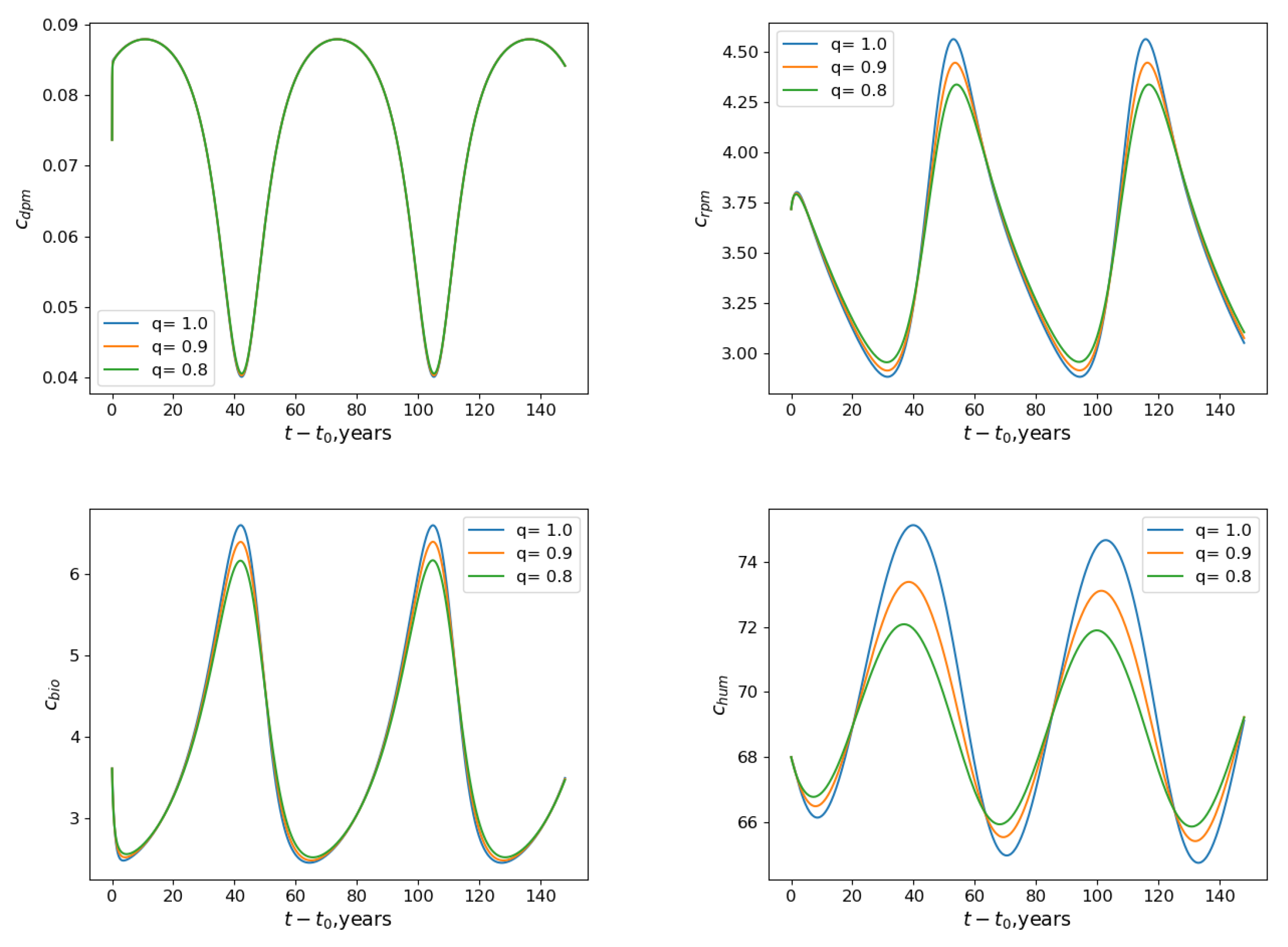
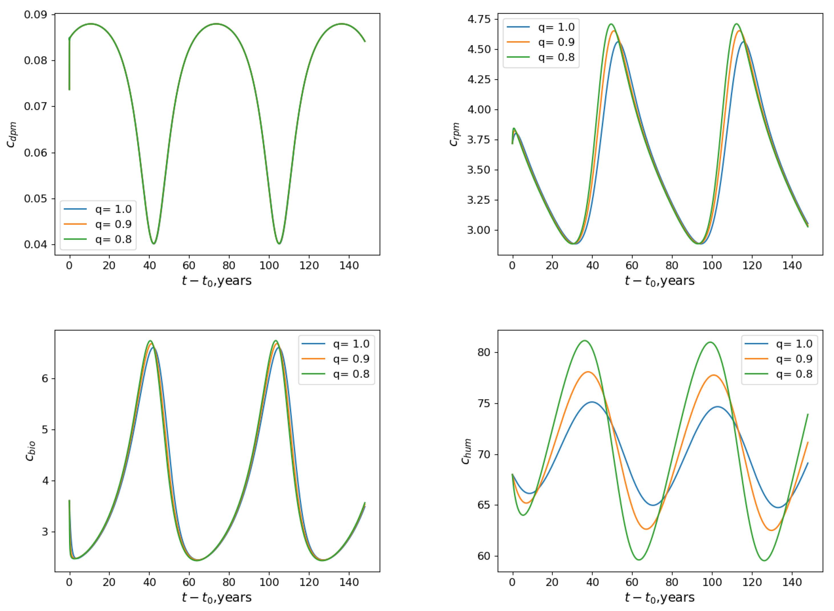
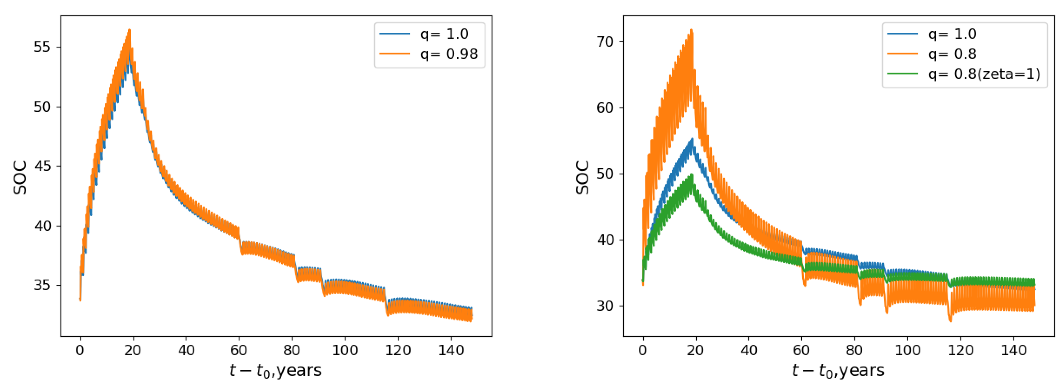
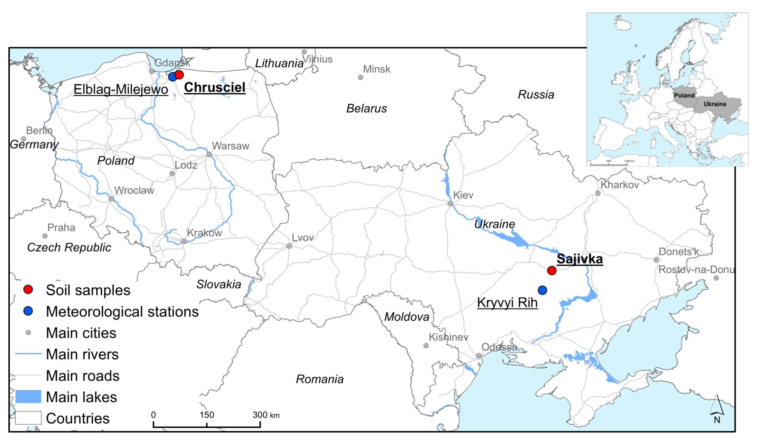
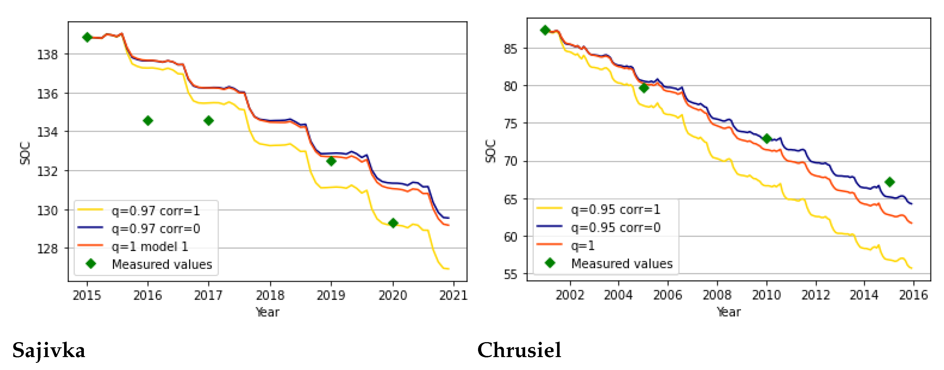
4.3. Ukrainian and Polish Scenarios

The proposed model was also applied to simulate SOC dynamics on the basis of data on the agrochemical and physical parameters of the soils in Ukraine and Poland. We selected two sites. For Ukraine, we chose the space point called “Sajivka”, located within an agricultural field. This field is characterized by Chernozem soil formed on loess with high content of carbonates under steppe vegetation. Chernozems are very fertile soils and very high agricultural yields can be obtained. A humid continental climate zone characterizes the site for which data on humus content, clay content, and soil density are available for the years from 2015 to 2020 (https://ismld.com.ua/ (accessed on 27 November 2022)). A weather dataset containing daily maximal, minimal, and average temperatures along with the amount of precipitation was obtained from ftp://ftp.ncdc.noaa.gov (accessed on 27 November 2022) for the weather station located in Kryvyi Rih city.

For Poland, the control point was selected from the database of the Polish Chief Inspectorate for Environmental Protection, which contains measurements of soil properties on a regular basis, every 5 years, since 1995, for a network of 216 control points located on arable land throughout the country (https://www.gios.gov.pl/chemizm_gleb/index.php?mod=monit (accessed on 20 December 2022.)). The site, called “Chrusciel”, is characterized by a fertile Luvisol (IUSS Working Group WRB (2022). “World Reference Base for Soil Resources, 4th edition”. IUSS, Vienna) originating from sandy loam. It is considered of high agricultural usefulness, with complexes (Saturnin Zawadzki (red): Gleboznawstwo. PWRiL, 1999. ISBN 83-09-01703-0.) suitable for the cultivation of sugar beet, wheat, red clover, alfalfa, winter rape, and faba bean. The point is under the climatic influence of the Baltic sea and is characterized by the following conditions: annual mean temperature $8.5{}^{\circ }$C, mean annual precipitation 710 mm, and growing season length 215 days. The choice of the site was based on its proximity to a meteorological station, Elblag-Milejewo (http://www.meteomanz.com (accessed on 20 December 2022)). Figure 4 presents the spatial distribution of the two points and

Table 5. Summary of the datasets from Ukraine.

Point	Clay Content, %	Humified Layer Depth, cm	Mean Temperature, °C	$\mathit{P}\left({\mathit{t}}_{\mathbf{0}}\right)$	Initial SOC, $\mathit{t}\mathit{C}/\mathit{ha}$
Sajivka	55.0	40	10.57	1.6296	138.8
Chrusciel	11.83	30	8.46	1.11616	87.36

contains their main characteristics.

4.4. Ukrainian and Polish Numerical Experiments

For both scenarios, as only data on humus content are available, we assume that in the initial moment of time, the SOC concentrations of all other compartments but the humidified one are equal to 0. Moreover, as the introduction of manure is not common in large-scale crop production, we consider $f\left(t\right)=0$. The representation of the density function $g\left(t\right)$ is given according to [4] in the form $g\left(t\right)=P\left(t\right)\widehat{g}\left(t\right)$, where $P\left(t\right)$ is the integral yearly value of $g\left(t\right)$ and $\widehat{g}\left(t\right)$ represents the distribution of $g\left(t\right)$ within the year. The value of $\widehat{g}\left(t\right)$, due to the lack of actual data, was taken equal to ${\widehat{g}}_{r\left(a\right)}\left(t\right)$ from Table 1 in [4] ($1/6$ for April, May, June; $1/2$ for July; 0 for other months). Net Primary Production (NPP) estimates (from the MOD17A3HGF.006 database of the NASA Earth Observation System (EOS) program; temporal range from 2015 to 2020. Application for Extracting and Exploring Analysis Ready Samples (AppEEARS)) in the considered points have been used to evaluate the annual values of $P\left(t\right)$ from the initial value $P\left(t_0\right)$, according to the formula $P\left(t_{n+1}\right)=P\left(t_0\right)NPP\left(t_{n+1}\right)/NPP\left(t_0\right)$ as in [4]. Given the hypothesis that, at the initial moment of time, the observed values of SOC compounds correspond to their values at a stable equilibrium [4], the value of $P\left(t_0\right)$ reported in Table 5 was calculated according to Equation (11) in [4], taking into account the considered assumptions

$$P\left(t_0\right)=12{\rho }^{\left(0\right)}\left(r\right)\delta k_{hum}{c}_{hum}\left(t_0\right)$$

(16)

The value of ${\rho }^{\left(0\right)}\left(r\right)=k_c\left(r\right)$ with $k_c\left(r\right)$ calculated as in [4]

$$k_c\left(r\right)=0.6\frac{N_p}{30}{\displaystyle \frac{e^{x\left(r\right)}}{1+e^{x\left(r\right)}}},x\left(r\right)=30{\displaystyle \frac{r-1}{r}}$$

with the number of months per year of bare soil set at $N_b=4$ for the Ukraine point from April to July, while $N_b=3$ for the Polish site, from August to October. The value of the DPM/RPM ratio r was equal to $1.44$, which corresponds to agricultural crops.

We assume a sufficient moisture supply for the site “Sajivka” as it is located within the lands of irrigation systems, and we assume the respective field to be irrigated. The irrigation system is not taken into account by the RothC model; therefore, it is necessary to add the amount of water due to the irrigation of the crops to the count of the monthly rainfall that occurred during the irrigation period. Therefore, we assume as a soil water deficit the amount of water added with irrigation, as in [28]. Consequently, the soil moisture deficit there should not be significant. For the “Crushiel” scenario, potential evapotranspiration (PET) assessments obtained using GLEAM remote sensing PET products (actual evaporation) [29] were used to evaluate the accumulated soil moisture function.

To assess the performance of different models and the errors between the real observed and predicted values, we use the modeling efficiency index (EF) and the root-mean-square error (RMSE) defined as

$$EF={\displaystyle \frac{{\sum }_{i=1}^n{\left(R_i-\overline{R}\right)}^2-{\sum }_{i=1}^n{\left(R_i-P_i\right)}^2}{{\sum }_{i=1}^n{\left(R_i-\overline{R}\right)}^2}}RMSE=\sqrt{{\displaystyle \frac{1}{n}}{\sum }_{i=1}^n{\left(R_i-P_i\right)}^2}$$

where R are the real SOC field observations and P are the SOC model simulations, n is the number of observations, and $\overline{R}$ is the mean. The EF values from 0 to 1 indicate that the model results are better than those using the mean values of observations and values below 0 are worse. The best-performing models are those with EF close to 1. For the RMSE, the values close to zero indicate that the simulated solution describes the data well. Some of the obtained numerical results are shown in Figure 5 and statistical performance is given in

Table 6. Statistical model indicators RMSE and EF, evaluated for the comparison of the fractional-order and RothC models in the Sajivka and Chrusciel sites.

	Sajivka			Chrusiel
	$q=0.97$, $corr=1$	$q=0.97$, $corr=0$	$q=1$	$q=0.99$, $corr=1$	$q=0.99$, $corr=0$	$q=1$
EF	0.851173	0.798365	0.808609	0.836487	0.922287	0.900954
RMSE	1.201889	1.398968	1.362967	3.044274	2.098715	2.369329

.

For the point "Sajivka", the solution that best matches the observed dynamics was obtained using the fractional-order model for $q=0.97$ and $\zeta (t,q)=t^{q-1}$, which reaches the best EF value $0.851173$ and RMSE value $1.201889$. We point out that the evaluation of the statistical indices in this case was carried out taking into consideration all the observed measured values of SOC, excluding the year 2018 as it represents an outlier. The use of the fractional-order model with $\zeta (t,q)=1$ yields slight but worse changes compared with the integer-order model in the studied cases with a 5-year simulation period.

For the point “Chrusciel”, the solution that best matches the observed dynamics was obtained using the fractional-order model for $q=0.95$ and $\zeta (t,q)=1$. Here, the use of the fractional-order model with $\zeta (t,q)=t^{q-1}$ yields worse changes compared with the integer-order model.

Simulation of the SOC dynamics for the Poland and Ukraine sites showed that the use of the fractional-order model with $\zeta (t,q)=t^{q-1}$ seems to correct the simulation dynamics in the cases when, with the best-known values of models’ parameters, the SOC content is overestimated by the integer-order model. Conversely, the choice of a fractional model with $\zeta (t,q)=1$ corrects the simulation dynamics in the cases when the SOC content is underestimated by the model predictions. In general, the use of fractional-order models introduces two added degrees of freedom, the q parameter and function $\zeta (t,q)$, which allows us to correct the SOC trend predicted by the classical model. The obtained results in terms of the statistical indicators EF and RMSE confirm the improved performance of the fractional model when compared with the integer-order model.

5. Conclusions

In this study, we formulated the fractional-order generalization of the continuous RothC model and studied the qualitative properties of its numerical solutions. The introduction of the Caputo derivative with respect to the time variable into the model reflects the case of fractal-structured soils in which carbon compartment-related reactions occur. As such an introduction requires the agreement of coefficients’ dimensions, we consider two possible forms of corresponding correction multipliers, obtaining two models with different behavior of the solutions.

The respective solutions were obtained by a finite difference scheme whose conditional stability was investigated. Because of the non-constant coefficients of the model, the usage of a fully numerical method is here justified by the high computational complexity of the exact solution’s discretization, which is the scheme that is widely and effectively applied for integer-order models and fractional-order models with constant coefficients.

The results of the fractional-order model’s application to several real-world scenarios with once-per-year measured SOC values show that it can be used to increase the accuracy of simulation by fitting the order of the fractional derivative. In the case of the simplest correction multiplier $\zeta (t,q)=1$, significant differences compared to the integer-order model were observed for the carbon compartments’ dynamics within the year. Thus, further studies with a higher frequency of SOC measurements are needed to identify the limits of such a fractional-order model’s usability.

For the Ukranian and Polish real-world scenarios, in the case of the multiplier in the form $\zeta (t,q)=t^{q-1}$, a decrease in SOC content compared with the integer-order model was observed. Conversely, an increase in SOC content compared with the integer-order model was obtained for $\zeta (t,q)=1$. As such a decrease can also be simulated by the changes in other models’ parameters, particularly the rate modifier $\rho \left(t\right)$, additional studies should be performed to distinguish real-world cases in which the influence of each of these parameters prevails.

As a future application, we will investigate the benefits of introducing the fractional-order derivatives for those compartmental models that explicitly consider the microbes’ influence on soil organic matter decomposition and on the long-term stabilization of carbon in soils [30].

References

1. Diele, F.; Luiso, I.; Marangi, C.; Martiradonna, A. SOC-reactivity analysis for a newly defined class of two-dimensional soil organic carbon dynamics. Appl. Math. Model. 2023, 118, 1–21. [Google Scholar] [CrossRef]
2. Coleman, K.; Jenkinson, D.; Crocker, G.; Grace, P.; Klir, J.; Körschens, M.; Poulton, P.; Richter, D. Simulating trends in soil organic carbon in long-term experiments using RothC-26.3. Geoderma 1997, 81, 29–44. [Google Scholar] [CrossRef]
3. Coleman, K.; Jenkinson, D.S. ROTHC-26.3: A Model for the Turnover of Carbon in Soil: Model Description and Users Guide: K. Coleman and DS Jenkinson; IACR: Santa Barbara, CA, USA, 1995. [Google Scholar]
4. Diele, F.; Luiso, I.; Marangi, C.; Martiradonna, A.; Woźniak, E. Evaluating the impact of increasing temperatures on changes in Soil Organic Carbon stocks: Sensitivity analysis and non-standard discrete approximation. Comput. Geosci. 2022, 26, 1345–1366. [Google Scholar] [CrossRef]
5. Marangi, C.; Diele, F.; Luiso, I.; Martiradonna, A.; Wozniak, E. SOC indicator of land-degradation: Responses of continuous and non-standard discrete RothC models to environmental changes. In Proceedings of the EGU General Assembly Conference Abstracts, Vienna, Austria, 23–27 May 2022; p. EGU22-5894. [Google Scholar]
6. Diele, F.; Marangi, C.; Martiradonna, A. Non-standard discrete RothC models for soil carbon dynamics. Axioms 2021, 10, 56. [Google Scholar] [CrossRef]
7. Parshotam, A. The Rothamsted soil-carbon turnover model—Discrete to continuous form. Ecol. Model. 1996, 86, 283–289. [Google Scholar] [CrossRef]
8. Pachepsky, Y.; Timlin, D. Water transport in soils as in fractal media. J. Hydrol. 1998, 204, 98–107. [Google Scholar] [CrossRef] [Green Version]
9. Kong, B.; Dai, C.X.; Hu, H.; Xia, J.; He, S.H. The Fractal Characteristics of Soft Soil under Cyclic Loading Based on SEM. Fractal Fract. 2022, 6, 423. [Google Scholar] [CrossRef]
10. Singh, A.; Das, S.; Ong, S. Study and analysis of nonlinear (2+1)-dimensional solute transport equation in porous media. Math. Comput. Simul. 2022, 192, 491–500. [Google Scholar] [CrossRef]
11. Priya, P.; Sabarmathi, A. Caputo Fractal Fractional Order Derivative of Soil Pollution Model Due to Industrial and Agrochemical. Int. J. Appl. Comput. Math 2022, 8, 250. [Google Scholar] [CrossRef]
12. Tanriverdi, T.; Baskonus, H.M.; Mahmud, A.A.; Muhamad, K.A. Explicit solution of fractional order atmosphere-soil-land plant carbon cycle system. Ecol. Complex. 2021, 48, 100966. [Google Scholar] [CrossRef]
13. Vieru, D.; Fetecau, C.; Ahmed, N.; Ali Shah, N. A generalized kinetic model of the advection-dispersion process in a sorbing medium. Math. Model. Nat. Phenom. 2021, 16, 39. [Google Scholar] [CrossRef]
14. Krasnoschok, M.; Pereverzyev, S.; Siryk, S.; Vasylyeva, N. Determination of the fractional order in quasilinear subdiffusion equations. Fract. Calc. Appl. Anal. 2020, 23, 695–722. [Google Scholar] [CrossRef]
15. Podlubny, I. Fractional Differential Equations; Academic Press: New York, NY, USA, 1999. [Google Scholar]
16. Samko, S.; Kilbas, A.; Marichev, O. Fractional Integrals and Derivatives; Gordon and Breach Science Publishers: New York, NY, USA, 1993. [Google Scholar]
17. Wheatcraft, S.; Meerschaert, M. Fractional conservation of mass. Adv. Water Resour. 2008, 31, 1377–1381. [Google Scholar] [CrossRef]
18. Gomez-Aguilar, J.; Miranda-Hernandez, M.; Lopez-Lopez, M.; Alvarado-Martinez, V.; Baleanu, D. Modeling and simulation of the fractional space-time diffusion equation. Commun. Nonlinear Sci. Numer. Simul. 2016, 30, 115–127. [Google Scholar] [CrossRef]
19. Wei, L. Global existence theory and chaos control of fractional differential equations. J. Math. Anal. Appl. 2007, 332, 709–726. [Google Scholar]
20. Matychyn, I. Analytical Solution of Linear Fractional Systems with Variable Coefficients Involving Riemann–Liouville and Caputo Derivatives. Symmetry 2019, 11, 1366. [Google Scholar] [CrossRef] [Green Version]
21. Garrappa, R.; Popolizio, M. Computing the matrix Mittag-Leffler function with applications to fractional calculus. J. Sci. Comput. 2018, 77, 129–153. [Google Scholar] [CrossRef] [Green Version]
22. Li, C.; Zeng, F. The Finite Difference Methods for Fractional Ordinary Differential Equations. Numer. Funct. Anal. Optim. 2013, 34, 149–179. [Google Scholar] [CrossRef]
23. Garrappa, R. Numerical solution of fractional differential equations: A survey and a software tutorial. Mathematics 2018, 6, 16. [Google Scholar] [CrossRef] [Green Version]
24. Zayernouri, M.; Karniadakis, G. Exponentially accurate spectral and spectral element methods for fractional ODEs. J. Comput. Phys. 2014, 257, 460–480. [Google Scholar] [CrossRef]
25. Langlands, T.; Henry, B. The accuracy and stability of an implicit solution method for the fractional diffusion equation. J. Comput. Phys. 2005, 205, 719–736. [Google Scholar] [CrossRef]
26. Hundsdorfer, W. Unconditional convergence of some Crank-Nicolson LOD methods for initial-boundary value problems. Math. Comput. 1992, 58, 35–53. [Google Scholar]
27. Rothamsted Experimental Station, Great Britain. Rothamsted: Guide to the Classical Field Experiments; AFRC Institute of Arable Crops Research: Harpenden, UK, 1991. [Google Scholar]
28. Di Bene, C.; Marchetti, A.; Francaviglia, R.; Farina, R. Soil organic carbon dynamics in typical durum wheat-based crop rotations of Southern Italy. Ital. J. Agron. 2016, 11, 209–216. [Google Scholar] [CrossRef] [Green Version]
29. Martens, B.; Miralles, D.; Lievens, H.; van der Schalie, R.; de Jeu, R.; Fernández-Prieto, D.; Beck, H.; Dorigo, W.; Verhoest, N. GLEAM v3: Satellite-based land evaporation and root-zone soil moisture. Geosci. Model Dev. 2017, 10, 1903–1925. [Google Scholar] [CrossRef] [Green Version]
30. Wieder, W.R.; Allison, S.D.; Davidson, E.A.; Georgiou, K.; Hararuk, O.; He, Y.; Hopkins, F.; Luo, Y.; Smith, M.J.; Sulman, B.; et al. Explicitly representing soil microbial processes in Earth system models. Glob. Biogeochem. Cycles 2015, 29, 1782–1800. [Google Scholar] [CrossRef] [Green Version]
Figure 1. From the top-left cell following the left-to-right direction: the numerical solutions c d p m , c r p m , c b i o , c h u m with respect to t t 0 for h = 0.02 in the case of periodic inputs ( ζ ( t , q ) = 1 ).
Mathematics 11 01677 g001
Figure 2. From the top-left cell following the left-to-right direction: the numerical solutions c d p m , c r p m , c b i o , c h u m with respect to t t 0 for h = 0.02 in the case of periodic inputs ( ζ ( t , q ) = t q 1 ).
Mathematics 11 01677 g002
Figure 3. Dynamics of SOC indicator in Scenario 3 for q = 1 and q = 0.98 . On the left: ζ ( t , q ) = t q 1 . On the right: ζ ( t , q ) = t q 1 (default), ζ ( t , q ) = 1 .
Mathematics 11 01677 g003
Figure 4. Locations of points with SOC data in Poland and Ukraine.
Mathematics 11 01677 g004
Figure 5. The values of SOC obtained for the integer-order and the fractional-order models (“corr = 0” means ζ ( t , q ) = 1 , “corr = 1” means ζ ( t , q ) = t q 1 ): left for the point “Sajivka”, right for the point “Chrusciel”.
Mathematics 11 01677 g005