Abstract
Despite achieving success in many domains, deep learning models remain mostly black boxes, especially in electroencephalogram (EEG)-related tasks. Meanwhile, understanding the reasons behind model predictions is quite crucial in assessing trust and performance promotion in EEG-related tasks. In this work, we explore the use of representative interpretable models to analyze the learning behavior of convolutional neural networks (CNN) in EEG-based emotion recognition. According to the interpretable analysis, we find that similar features captured by our model and state-of-the-art model are consistent with previous brain science findings. Next, we propose a new model by integrating brain science knowledge with the interpretability analysis results in the learning process. Our knowledge-integrated model achieves better recognition accuracy on standard EEG-based recognition datasets.
MSC:
68T07
1. Introduction
Electroencephalogram data are used to measure oscillations in the brain and can reflect the synchronized activity of neurons. These oscillatory changes are thought to be related to cognitive processes, including perception, attention, learning, memory, and emotion. Out of the many EEG-related tasks, emotional identification is the most popular. Emotion identification is the act of identifying the emotional state of individuals by obtaining physiological or non-physiological signals, which is an important part of emotion computing. Through emotion identification, we can obtain individual emotional states relatively accurately without subjective interference in some practical scenes, such as judicial, medical, etc. As a physiological signal, EEG has the advantage of being difficult to hide and disguise compared with intuitive facial recognition. Therefore, using EEG to recognize emotions can help us better understand emotions from the physiological perspective and establish the cognitive connection between EEG physiological signals and emotions.
In the past decade, machine learning models, especially deep learning methods, have achieved an exciting breakthrough in EEG-based emotion recognition. Unfortunately, although existing work improved the recognition accuracy greatly, there is still growing concern about their black-box nature. Simply speaking, these methods cannot provide sufficient clues on their internal learning actions. There are still many unanswered questions surrounding their models, including but not limited to: Why these models can be successful? Which features are most effective?
To our knowledge, increasing the interpretability is especially important to EEG-related tasks as to the following aspects [1]: (i) understand which features better discriminate the investigated classes and check that the learning system does not rely on artifactual sources; (ii) increase the insight into the neural correlates of the model that underlies learned behaviors; (iii) interpretability analysis can also shed some light on model design, driving us to design novel learning models. Despite its many advantages, interpretability analysis for EEG-related tasks is still in its infancy [2]. The biggest reason behind it is the complexity of EEG data, which brings the difficulty of EEG tasks based on these data. First, as a non-invasive signal obtained along the scalp, EEG suffers from a low signal-to-noise ratio (SNR) [3]. Second, EEG is generally recorded using tens to hundreds of electrodes simultaneously, and the sampling time usually exceeds a few seconds in each trial. Thus, the original feature dimension of an EEG sample is high. However, the number of samples in the EEG-related task is not high, which would lead to a very low initial ratio of samples to features. Third, the inherent variabilities in brain anatomy, head size, and dynamics across trials/subjects considerably limit the generalizability of EEG analyses across subjects and even across trials within a single subject performing a single task. All of these lead to problems such as over-fitting and poor generalization when building a deep learning model on EEG data and also increase the difficulty of studying the interpretability of learned models. To the best of our knowledge, although some recent efforts have been dedicated to explaining the behaviors and decisions of deep networks in other fields, few existing works attempt to provide an overview of the representative interpretable models used for analyzing underlying behaviors of deep learning models on EEG data. In the conference version of our work [4], we tried to use two interpretability methods, Local Interpretable Model-agnostic Explanations (LIME) [5] and Gradient-weighted Class Activation Mapping (Grad-CAM) [6], to study the learning behaviors of a CNN model. However, experiments were only carried out on one dataset, and there was no attempt to integrate brain science knowledge to obtain a better recognition model.
To sum up, the contribution of this work is three-fold: (i) we propose to use two representative interpretability approaches to study the EEG-based emotion recognition models; (ii) according to the interpretability analysis, we increase the understanding of which features better discriminate the target classes. We also find that the features learned by the model are consistent with previous brain science findings; (iii) by integrating the knowledge from brain science, our model achieves better recognition accuracy.
The rest of the article is organized as follows: Section 2 briefly reviews the typical studies about interpretability methods and knowledge-integrated EEG models; Section 3 details the structure of the proposed model and interpretability algorithms conducted; Section 4 describes all the experimental settings and processes; including dataset, parameters, comparative methods and comprehensive analysis of results, and Section 5 concludes by outlining the key contents and contributions overall.
2. Related Works
To date, no studies have systematically used interpretability approaches to study the deep learning models on EEG data and integrate neuroscience knowledge into the learning process of their model. Therefore, in this section, we will first present the current state of research on interpretability methods, then we will present some work on designing models using theories related to neuroscience.
2.1. Interpretability Methods for Deep Learning
Deep neural networks are often considered black boxes. In many research studies, despite the fact that the proposed model shows great performance, the author is usually unable to accurately interpret the internal behaviors of the model. Therefore, the ability to interpret deep learning models is essential for further research of specific tasks. It can help researchers understand the model, thereby better optimizing the model and improving the theoretical support of the proposed method. Generally, there are two types of interpretable methods based on the timing of interpretation, passive methods, and active methods. The task of the passive method is to explain a model that has been trained and generally does not affect the main structure of the interpreted model; for the active method, the task has changed from explaining a black box model with already good performance to building both interpretable and well-performed model, which means the balance between interpretability and target task performance must be considered before modeling, so as to significantly increase the difficulty of modeling compared with building a regular convolutional neural network (CNN). Thus, most of the studies consider the passive methods at first, where the most common ones are visualization-related methods [7]. Ribeiro et al. [5] proposed an algorithm, LIME, that interprets the prediction of the target classifier or regressor by approximating it locally with a naturally interpretable model. Class Activation Mapping (CAM) [8] is a general technique that can be utilized to visualize the predicted class scores on any given image, highlighting the discriminative object parts detected by the CNN. As a generalization of CAM, Grad-CAM [6] allows the CNN of any structure to be visualized without modifying the network structure or retraining. Different from gradient-based CAM and Grad-CAM, Deep Learning Important Features (DeepLIFT) [9] is a method for decomposing the output prediction of a neural network on a specific input by backpropagating the contributions of all neurons in the network to every feature of the input. For active methods, they usually add extra components in the interpreted model beforehand or extend the training framework to synchronously intervene in the training of the target model. Li et al. [10] and Chen et al. [11] added a prototype layer to the model to explain a prediction by the learned prototypes. Weinberger et al. [12] and Plumb et al. [13] utilized an interpretability regularizer to regularize the prediction model, and the latter additionally implements prior knowledge and a feature learning model for alternate training with the predictive model. Similarly, Wojtas et al. [14] proposed a dual-net architecture composed of an operator and a selector, both of which are Multilayer Perceptrons (MLPs) for predicting and feature selecting, respectively. After alternate training, the optimal feature subset and the importance order of the features are learned, and the operator can predict the test data according to the optimal feature subset.
Before us, there were some other EEG-related tasks that used interpretability methods to test and verify their proposed models that are good enough. In their approach, the interpretability part is just an embellishment. The application of a deep neural network (DNN) with layer-wise relevance propagation (LRP) on EEG data was first proposed by Sturm et al. [15], in which the LRP-derived scalp topography maps reveal the relevance between single test data and the decision of DNN. Vilamala et al. [16] resorted to multitaper spectral analysis to create visually interpretable images of sleep patterns from EEG signals as inputs to a deep convolutional network trained to solve visual recognition tasks. Qing et al. [17] proposed a coefficient-based method based on machine learning using EEG signals to solve the problem of insufficient understanding of emotional stimulation mechanisms in traditional research. This method not only outperforms the benchmark algorithm in accuracy but can also better explain the emotion activation process. Some works implemented visualization heatmaps to highlight the importance of EEG channels, for example, Li et al. [18] used Grad-CAM to select channels before training their model, and the interpretability part in TSception [19] shows that the saliency maps [20] drew from the network match the existent cognitive neuroscience theory. More recently, Ludwig et al. [21] put forward a new EEG decoding pipeline (EEGminer) with learnable filters, which can discover interpretable features of brain activity. Using the parameters of trainable generalized Gaussian filters as an interpretable tool, they effectively revealed the features of channel connectivity and the magnitude behind brain activity. Although the above works involve interpretability, their main purpose is to propose a model with better performance, in which interpretability is merely used as a supplementary part to support the model, lacking systematicness and comprehensiveness.
2.2. Knowledge-Integrated EEG Model
Hemispheric lateralization refers to the phenomenon of specialization or asymmetry in the division of labor between the left and right hemispheres of the brain. Jiang et al. exploited the hemispheric lateralization of the human brain in the proposed deep framework to extract more compact and class-dependent brain features [22], and the experiment results of the model on Object Category-EEG and ImageNet-EEG dataset were better than those of the state-of-the-art. Zhong et al. proposed a network called RA-BiLSTM that extracted additional information at the regional level to strengthen and emphasize the differences between the two hemispheres [23]; it achieved the best results on the classification of ImageNet-EEG. Ding et al. proposed a multi-scale convolutional neural network and learned discriminative global and hemispherical representations using asymmetric spatial layers [19]; the classification accuracy on DEAP and MAHNOB-HCI exceeded most traditional machine learning and deep models. In 2022, Zhong et al. proposed a novel bi-hemispheric asymmetric attention network combining a transformer structure with the asymmetric property of the brain’s emotional response [24]; the results of this model were better than both classical machine learning and state-of-the-art deep learning methods on the DEAP. Although these works tried to incorporate some prior knowledge into model training, we found that all of these existing works are based on hemispheric lateralization, while none of the other knowledge was integrated into the models.
3. Methods
We first build a simple convolutional neural network Simple Asynchronous Convolutional Neural Network (SACNN), then we use interpretability methods to analyze the trained SACNN. Finally, as shown in Figure 1, we propose a new method by integrating neuroscience knowledge into EEG emotion classification.
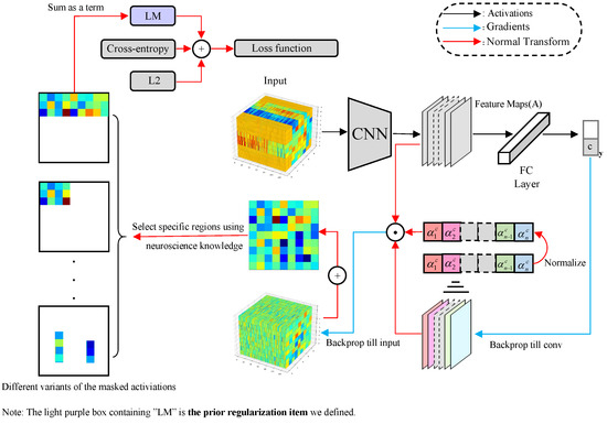
Figure 1.
Knowledge-Integrated Region-wise Loss Construction.
3.1. A Simple Model
In this section, we construct a simple CNN-based model SACNN. SACNN consists of four convolutional layers, two dropout layers, and three fully connected layers. Among them, the convolution kernel size of the four convolution layers is , the padding is 1, the convolution kernel step of the first and third convolution layers is 1, and the kernel step of the second and fourth convolution layers is 2. The details of the model are given in Table 1.

Table 1.
The structure of SACNN.
In order to extract the spatial information of EEG, we map the one-dimensional EEG channel onto the two-dimensional grid to get the input of SACNN. For a sample , n denotes the number of electrodes, and t is the sampling points of the EEG sample; in our method, t is 128. By following existing work [25], as shown in Figure 2, we map the EEG channels onto a grid according to the international 10–20 system. Finally, the size of the SACNN input is .
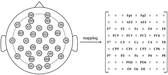
Figure 2.
Electrodes are mapped onto a matrix according to their relative spatial positions.
3.2. Interpretability Algorithm
3.2.1. LIME
We try to use LIME to explore the region-level importance of EEG data extracted and strengthened by the CNN model. For the image classification task, LIME assumes an interpretable representation as a binary vector indicating the “presence” or “absence” of a contiguous patch of similar pixels. In detail, it sets each segmented region as a super-pixel and inputs every possible combination of super-pixels into the learned model to obtain the probability of each combination. The obtained probability is used as a label for the explanation model. Finally, the contributed value of each super-pixel is learned as the weights of a sparse linear model via least squares by Lasso [26].
For our problem, we simply use two types of segmentations in our experiment. The first one is the top, middle, and bottom regions, and another is the left, middle, and right regions. We adopt these two regional divisions because they are consistent with the natural divisions of the brain cortex and are commonly used in the existing EEG studies [27,28]. Each of the regions is set as an instance being explained; its original representation is denoted as . We use to denote a binary vector for its interpretable representation where d is three because there exists three regions/super-pixels in each regional division. The possible combination of super-pixels is denoted as , and it includes eight cases: {1, 1, 1}, {1, 1, 0}, {1, 0, 1}, {0, 1, 1}, {1, 0, 0}, {0, 1, 0}, {0, 0, 1}, {0, 0, 0}. One means the corresponding region is present, while zero means it is absent.
Given a sample , we recover the sample in the original representation and input it into the trained model and obtain the probability of the predicted label for the current EEG data, which is used as the label for the explanation model. The contributed value is the weight of a sparse linear model , which is learned via least squares by Lasso. We use the locally weighted square loss as , as defined in Equation (1). We let be an exponential kernel defined on the distance function with width, which is used as the complexity measure for each combination. Here, is equal to 0.25, and is defined as {1, 1, 1}.
3.2.2. Grad-CAM
Given an EEG sample , we feed into the trained convolutional network to find its emotion category . We first derive the value of corresponding to the label c, then get the k-th activation map of the convolutional layer, and calculate the derivative of to derived from the k-th feature map of a convolutional layer. Finally, we globally sum the flowing back gradients over which the width is m and height is n to obtain the feature map local importance weights: :
Using as the weight of , through Equation (4), we get the weighted sum of the feature maps. Then, is up-sampled to the same spatial resolution as the input.
3.3. Knowledge-Integrated Region-Wise Loss
As shown in Figure 1, we first input the samples into SACNN, then use the interpretability algorithm to extract the decision basis of the model, and finally, according to the chain derivation rule, we force the optimization direction of the neural network to match the neuroscience knowledge.
Following Grad-CAM, we first derive the of the feature map from the last convolutional layer; here, we input to the untrained model f instead of , and c is the ground truth label of , and we obtain the normalized weight .
According to current research in neuroscience, different brain regions have different effects on emotions. Therefore, we design a term in loss function to enforce that the input contribution to the model matches the widely accepted neuroscience knowledge.
For the feature map , we first obtain the derivative of with respect to , and then obtain the derivative of with respect to . Since the importance of different feature maps to is inconsistent, we multiply with the above two items to locate the input . In order to obtain the importance of different spatial locations, after the sigmoid, we average the value along the sampling point dimension to get :
We define a matrix as a mask matrix, where , when is 1, it means that the electrode information at the corresponding position is selected, and vice versa. Using this mask, we design several different variants to strengthen different locations of the EEG signal, e.g., the left frontal lobe is associated with positive emotions. Finally, we get the regularization terms :
Finally, put , cross-entropy loss function , and regularization together as the new loss function of SACNN, the coefficient of the parameter is p, and q is the parameter of the prior regularization item .
4. Experimental Results
We first train SACNN on multiple datasets and then analyze the model with interpretability methods. For each dataset, we obtain ten models with ten-fold validation and select the model with the median accuracy on the test set for interpretability analysis. It is worth mentioning that we also compare the explanations result of the selected one with the others, and we find they are consistent with each other.
4.1. Experimental Setting
Here are the main experiments we design and conduct for interpretability analysis. First, we use LIME to obtain the contributed values of each region in two manually determined divisions based on two different CNNs on two datasets. With the same models and divisions above, we additionally calculate the accuracy of each region for validation. Second, we implement Grad-CAM on SACNN on all three datasets. We select the channels with high or low average values in the heatmaps derived from Grad-CAM and compute their accuracies. Finally, we train and test six variants of our proposed knowledge-integrated model on two datasets. For comparison, an active method is adopted with the same datasets.
4.2. Dataset
In this paper, we use three datasets for experiments, namely DEAP, MAHNOB-HCI, and SEED.
DEAP describes the recordings of EEG for 32 participants while they watched 40 one-minute-long excerpts of selected videos [29]. Each experiment included a stimulation of 60 s and a pretrial baseline of 3 s, and the preprocessed data have been downsampled to 128 Hz by the DEAP team [30]. After watching each video, the arousal and valence of subjects were measured using the self-reported Self-Assessment Model (SAM) scale; here, arousal is defined as the degree to which an individual is excited (e.g., high and low) while valence is defined as the polarity of emotion [31]. For arousal, the subjects would rate the video on a scale of 1–9, with 1 being boring and 9 being exciting. Regarding valence, the subjects would again rate the video on a scale of 1–9, with 1 being unpleasant and 9 being pleasant.
MAHNOB-HCI is a database for the automatic analysis of human emotions, including EEG and peripheral signals from 30 participants while watching 20 videos [32]. Three subjects lost data records, and two subjects had incomplete data records. Each video clip lasts 34–117 s, and the EEG sampling frequency is 512 Hz; in addition, the beginning and end of each video clip has 30 s as the baseline. After watching videos, participants were asked to report their felt arousal and valence using the SAM scale.
The SEED dataset includes EEG signals from 15 subjects during watching 15 movie clips. The sampling frequency is 200 Hz, and the duration of each film clip is approximately 4 min. The 15 movie clips are divided into three types according to the emotion expected to trigger, which are negative, neutral, and positive. Each type of clip accounts for one-third of the total number of clips. The participants were told to report their emotional reactions to each film clip by completing the questionnaire immediately after watching each clip [33,34]. Unlike DEAP and MAHNOB, the SEED dataset does not provide arousal and valence labels but only provides one label named emotion and divides the data into three categories.
4.3. Data Preprocessing and Parameter Setting
First, we apply baseline removal to eliminate the interference of the EEG signals in a relaxed state, according to the experiment [35]. For different datasets, the duration of a trial varies. Consistent with most existing works, we partition each trial of EEG signal flow into a set of samples, where each sample contains 128 sampling points so that different databases can work on the same model. For a sample, we convert the recorded EEG signals into a matrix with a shape of , where the n of DEAP, MAHNOB, and SEED is 32, 32, and 62, respectively. Finally, through Figure 2, we get the input of the model with the size . For DEAP and MAHNOB, the subject‘s self-reported arousal and valence values are divided into two categories as the labels according to the threshold value 5; those below 5 are 0, and others are 1. As we described before, the SEED dataset only has labels corresponding to the polarity of emotion, which is the valence dimension. However, it includes three categories, negative, neutral, and positive. In order to make its experimental results comparable with those of other datasets, we only use the data with negative and positive labels to train and test models.
In our model, cross-entropy is used as the loss function, and stochastic gradient descent (SGD) is applied for backpropagation; the momentum factor of SGD is 0.9. We use SELU as the activation function, the learning rate value is initialed to , and multiplied by 0.1 every 30 epochs. The training time of the network is 80 epochs. For each dataset, we divide the subsets in the trial dimension and divide all the trials of each person into ten folds according to the time order and combine, and finally, ten-fold cross-validation is used to train and test the constructed model. We use the L2 penalty and dropout layer to reduce the overfitting of the model; the L2 weight of dataset DEAP, SEED, and MAHNOB-HCI are , , and , respectively, and the drop rate is 0.3.
4.4. Comparative Methods
In our experiments, we use two comparative methods that are TSception [19] and a dual-net model [14]. TSception is one of the state-of-the-art (SOTA) EEG models, for which we conduct interpretability analysis on it for comparison with our proposed SACNN. The dual-net model is an active interpretability model, and we take it to compare the classification accuracy with SACNN so as to find out whether it is able to promote the classification performance in an active way.
TSception [19] is a novel multi-scale temporal-spatial convolutional neural network for EEG emotion recognition, which has achieved good performance in several public datasets. TSception consists of dynamic temporal, asymmetric spatial, and high-level fusion layers. The dynamic temporal layer consists of multi-scale 1D convolutional kernels whose lengths are 1/2, 1/4, and 1/8 of the sampling rate of EEG, respectively, and the asymmetric spatial layer takes advantage of the asymmetric EEG patterns for emotion, learning the discriminative global, and hemisphere representations. The learned spatial representations are finally input into a high-level fusion layer. In order to maintain the basic structure of TSception well and analyze the individual contribution of each region explicitly, we reconstruct the spatial layer and divide it into two modes, vertical (top/middle/bottom) and horizontal (left/middle/right), as shown in Figure 3. For each mode and its corresponding division, the spatial layer consists of multi-scale 1D convolutional kernels whose lengths are the number of EEG channels in each region. For every single input, we reorder the EEG channels separately by their spatial location in each division so as to keep the electrodes in a region adjacent. The updated version of TSception with both structures can achieve similar results with the original version of TSception (93% vs. 95% in DEAP and 97% vs. 99% in MAHNOB-HCI). In both versions, cross-entropy is used as the loss function, and stochastic gradient descent (SGD) is applied for backpropagation. The initial learning rate is set to , and the drop rate of the dropout layer is 0.5. The number of training epochs is 200 in DEAP and 100 in MAHNOB-HCI.
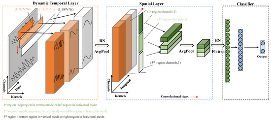
Figure 3.
Diagram of the updated version of TSception.
The novel dual-net architecture is proposed by Wojtas et al. [14], consisting of an operator and selector for the discovery of an optimal feature subset of a fixed size and ranking the importance of those features in the optimal subset simultaneously. It is an active interpretability method. In deployment, the selector generates an optimal feature subset and ranks feature importance, while the operator makes predictions based on the optimal subset for test data. In their experiment, MLPs (CNNs) of the sigmoid (ReLU) neurons are employed to carry out the operator net, and MLPs with the sigmoid neurons are employed for the selector net in the dual-net architecture. For training MLPs (CNNs), the Adam optimizer (Adam with Nestrov momentum for the operator net) is adopted via the stochastic gradient descent (SGD) procedure. At first, we try to implement the given dual-net on DEAP and SEED datasets with the same preprocessed procedure as our experiments above, which is using raw data as input and splitting the training and test sets by 10-fold cross-validation. We use the optimal hyperparameters on Binary Classification [36] for the MLP operator and those on the Yale dataset [37] for the CNN operator. However, it turns out that both of the two kinds of models did not work, they did not fit, and all the predictions tended to a single label. We deduce that it is not appropriate to directly use MLP as the classifier for raw EEG signals because of their high signal-to-noise ratio (SNR). As for the CNN operator, it is not suitable to use a two-dimensional spatial kernel for EEG series as well. In addition, the random batch sampling method cannot guarantee that the large training set is traversed enough for learning. Therefore, in order to maintain the basic structure of the dual-net, we change our input from raw EEG to extracted differential entropy (DE) and conduct the experiment only on the MLP operator with SELU.
4.5. Results
4.5.1. Analysis with LIME
For each dataset, we report the average contributed value of each region obtained from the test data for our proposed simple model (SACNN) and TSception [19] in both valence and arousal dimensions, e.g., Figure 4. The horizontal coordinate corresponds to the video list and the vertical coordinate is the contributed value. The first two columns correspond to the results in the top/middle/bottom division, and the last two correspond to those in the left/middle/right division, each of which contains the results of our model in the left and those of TSception in the right. The first row shows the results whose ground truth labels are 0; the second row shows those labels that are 1; and the third row gives the results without distinguishing which label the sample belongs to. In other words, it contains both cases.
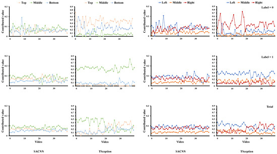
Figure 4.
The average contributed value of each region obtained from the test data of the DEAP dataset in the valence dimension.
We also provide classification accuracy when the information of specific regions is kept and others are masked out on the test data of each dataset for our model and TSception in both valence and arousal dimensions, e.g., Figure 5. Simply speaking, we only keep the information of a certain region in each sample and set the others to zero. Then we input all samples from the test data into the learned model and obtain accuracy. We first conduct experiments on the DEAP dataset. From Figure 4, we can find that although the structure of SACNN and TSception are different, the LIME analysis results in similar contributions of each region across them. For the valence dimension in Figure 4, we can find that the middle part in the top/middle/bottom division has a greater contribution to the high valence (label = 1) in both models. This is due to the fact that T7 and T8 of the temporal lobe are located in this region. The left part in the left/middle/right division has more contribution to high valence in both models as well. As we know, asymmetry between the hemispheres of the brain is related to emotions. A relative right frontal activation is associated with withdrawal stimuli or negative emotions; and a relatively greater left frontal activation is associated with positive emotions, such as joy or happiness [27]. These results are consistent with our observation in the LIME analysis. If we simply compare the classification accuracy of each region in the two models, it is seen that there is a difference between them, which is mainly caused by the different infrastructures of the two models. However, when we focus on the areas significantly relevant to emotion, they are similar though. In Figure 5, we can find the middle part in the top/middle/bottom division achieves better accuracy than other parts on high valence in both models. The left part in the left/middle/right division obtains the highest accuracy on high valence, while the right part obtains the highest accuracy on low valence in both models as well, which are all consistent with the contributed value obtained by LIME.
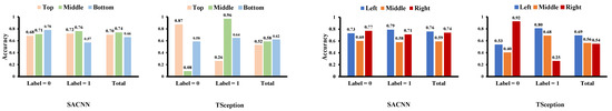
Figure 5.
The classification accuracy of each region on the test data of the DEAP dataset in valence dimension.
In Figure 6, we report the average contributed value of each region obtained from the test data of the DEAP dataset in the arousal dimension. From the existing research, the right hemisphere, especially the parietal lobe, is important in activating arousal systems, right dominance on P3, and late positive potentials over the parietal lobes appear during high arousal [38]. In our results, in the arousal dimension, it is observable that the right part in the left/middle/right division in SACNN and the bottom part in the top/middle/bottom division in TSception contribute more to high arousal. This is also consistent with the existing conclusions of brain science. The accuracy of each region is shown in Figure 7. Although the regional accuracies in the two models are not exactly the same due to the different structures of the models, we can still find out that the classification accuracies of different regions of the two models are basically the same in total. For example, the middle region is the highest in the top/middle/bottom division, while the middle is the lowest in the left/middle/right division in both models.
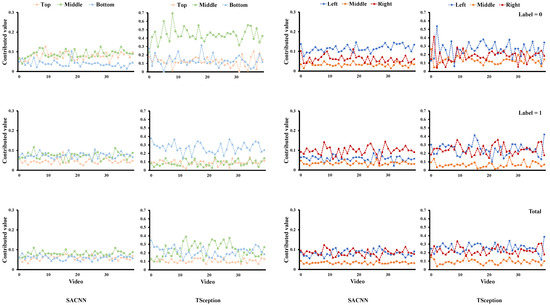
Figure 6.
The average contributed value of each region obtained from the test data of the DEAP dataset in the arousal dimension.
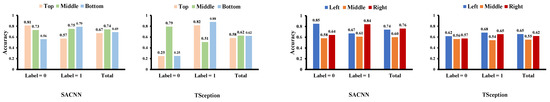
Figure 7.
The classification accuracy of each region on the test data of the DEAP dataset in the arousal dimension.
In Figure 8, we display the average contributed value of each region obtained from the test data of the MAHNOB-HCI dataset in the valence dimension. The horizontal coordinate corresponds to the video list in MAHNOB-HCI, which is different from the list in DEAP. Consistent with the results in the DEAP dataset, we can find the middle part in the top/middle/bottom division has a greater contribution to the high valence in both models, corresponding to which the middle part in the top/middle/bottom division achieves better accuracy than the other parts on high valence in both models in Figure 9. Although in SACNN, the line of left and right intertwine together, the left part and the right part in the left/middle/right division have overwhelmingly more contributions to high valence and low valence in TSception, respectively. Additionally, in Figure 9, the left part in the left/middle/right division obtains the highest accuracy on high valence, and the right part obtains the highest accuracy on low valence in both models. Thus, these results can be considered in line with the results in the DEAP dataset.
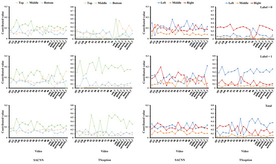
Figure 8.
The average contributed value of each region obtained from the test data of the MAHOB-HCI dataset in the valence dimension.
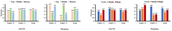
Figure 9.
The classification accuracy of each region on the test data of the MAHNOB-HCI dataset in the valence dimension.
For the arousal dimension in Figure 10, it is clear that the middle part in the top/middle/right division contributes the most to low arousal in both models. In Figure 11, the middle part in the top/middle/bottom division obtains higher accuracy than the other two on low arousal in both models as well. Additionally, we can find that there are many other similarities in the regional accuracies across the two models. In the top/middle/bottom division, apparently, the orders of the accuracies of the three regions in the two models are identical when arousal is low (label = 0), showing that the top part is the highest, then the bottom, and the middle is the last. In the left/middle/right division, the orders are the same as well when label = 0 and in total, where the right part reaches the highest and the middle is the lowest.
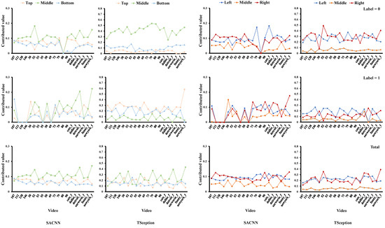
Figure 10.
The average contributed value of each region obtained from the test data of the MAHNOB-HCI dataset in the arousal dimension.
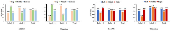
Figure 11.
The classification accuracy of each region on the test data of the MAHNOB-HCI dataset in the arousal dimension.
4.5.2. Using Grad-CAM to Select Channels
We use Grad-CAM to select channels with SACNN on all three datasets. For each sample in the training set, we set the Grad-CAM value of each channel as the importance value of this channel and then sort them. Then we separately sum all the ranking results on each label to get the final ranking of each channel, respectively. We provide the classification accuracy on the test data when the specific channels (top 10 vs. last 10) are kept, and the others are masked out in Table 2. From the results, we can find that Grad-CAM could help us select those important channels leading to higher classification accuracy in all three datasets.
Table 2.
The classification accuracy of the top/last 10 important channels on the test data obtained by Grad-CAM of the three datasets with different labels.
4.5.3. Results of Knowledge-Integrated Model
As we described before, we propose a knowledge-integrated method by integrating brain science knowledge into the interpretability analysis of our simple convolutional neural network. In our method, we define a mask , which helps us to strengthen the corresponding contribution from a particular brain region to emotion recognition. Specifically, in our experiment, we consider six versions of masks, as shown in Figure 12, including the left frontal lobe, the left hemisphere, the right frontal lobe, the right hemisphere, the frontal lobe, and seven important electrode sites for positive emotion. The seven important locations include the channels of FC3, C3, CP3, P3, C4, CP4, and P4. The parameter q of the prior regularization item is 1.
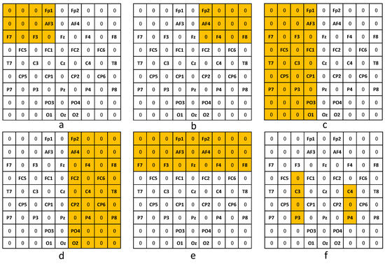
Figure 12.
Different variants of the mask . Here, the yellow means the channels are selected in the corresponding variant mask, (a) left frontal lobe, (b) right frontal lobe, (c) left hemisphere, (d) right hemisphere, (e) frontal lobe, and (f) seven important electrode sites.
As shown in Table 3, we give the average results for the 10-fold experiment of the proposed baseline model, its six variants, and the active model. From the results, we could find our proposed model shows better classification accuracy compared with the active model. More than that, we can also find the results are also in line with our expectations. The left frontal lobe and the left hemisphere are associated with positive emotions; and the right frontal lobe and the right hemisphere are associated with negative emotions. Thus, the first and second variant models show better recognition performance on high valence, while the third and fourth variant models show better recognition performance on low valence. If the frontal lobe is strengthened, the model will show better recognition performance in both cases. Zhao [39] performed the ERC algorithm using LSTM as the base regressor on EEG features with feature selection and ranking and found that the seven electrode sites, CP4, C4, P3, C3, P4, FC3, and CP3, are associated with positive emotion. Through the sixth variant models, we find that after strengthening these seven channels, the model really achieves better results on positive emotions.
Table 3.
The results of the experiment.
4.6. Discussion
In this section, we implement LIME to analyze the regional-level importance of EEG data on emotion-recognition CNNs, from which we discover that despite different structures of the models, the discriminative features learned for classification become similar. They also show consistency with the findings of emotion recognition in brain science, such as the well-acknowledged theory of brain asymmetry: a relative right frontal activation is associated with withdrawal stimuli or negative emotions; and a relatively greater left frontal activation is associated with positive emotions, such as joy or happiness. In addition, we try to use Grad-CAM to select the significant channels that contribute to specific emotion labels. It shows that the top-ranked channels with high-importance values outperform the last-ranked ones. We also propose a new model by integrating brain science knowledge with the interpretability analysis of SACNN, which achieves better accuracy than SACNN and the comparative active model. Overall, our results strengthen and validate the acknowledgments of emotion-recognition CNN models’ learning behaviors and enhance the credibility of the predictions provided by them.
5. Conclusions
Over the years, deep learning has broken records in many fields in a black-box manner. It also includes the field of EEG-based emotion recognition. However, now, more and more people realize that breaking records with increasingly complex models is not enough. We need to explore the potential reasons why the model is effective. On the one hand, it can avoid the model from just fitting to some noise that has nothing to do with emotion. On the other hand, it can give us useful inspiration for designing models. In this paper, we conduct a series of experiments with two generally used interpretable models on three datasets. Although the learning processes are not completely identical for the classification models with different structures, both models capture similar features that are also consistent with previous brain science findings. Moreover, by integrating the knowledge from brain science with the interpretability analysis results in the learning process, we propose a new model that achieves better recognition accuracy than the compared active model. In the future, we will seek to propose a more effective emotion classification model based on the interpretability method.
Author Contributions
Conceptualization, S.Z.; Methodology, S.Z.; Software, Y.Z. and C.C.; Writing—original draft, Y.Z. and C.C.; Writing—review & editing, Y.Z. and S.Z.; Supervision, S.Z. All authors have read and agreed to the published version of the manuscript.
Funding
This research was funded by Natural Science Foundation of Guangdong Province (2019A1515011181), Science and Technology Innovation Commission of Shenzhen under Grant (JCYJ20190808162613130) and National Natural Science Foundation of China (62002230).
Institutional Review Board Statement
Not applicable.
Informed Consent Statement
Not applicable.
Data Availability Statement
Publicly available datasets were analyzed in this study. DEAP, MAHNOB and SEED can be found here respectively: https://www.eecs.qmul.ac.uk/mmv/datasets/deap/download.html, accessed on 10 January 2023; https://mahnob-db.eu/hci-tagging/; https://bcmi.sjtu.edu.cn/home/seed/index.html, accessed on 10 January 2023.
Conflicts of Interest
The authors declare no conflict of interest.
References
- Borra, D.; Fantozzi, S.; Magosso, E. Interpretable and lightweight convolutional neural network for EEG decoding: Application to movement execution and imagination. Neural Netw. 2020, 129, 55–74. [Google Scholar] [CrossRef] [PubMed]
- Shahroudnejad, A. A survey on understanding, visualizations, and explanation of deep neural networks. arXiv 2021, arXiv:2102.01792. [Google Scholar]
- Roy, Y.; Banville, H.; Albuquerque, I.; Gramfort, A.; Falk, T.H.; Faubert, J. Deep learning-based electroencephalography analysis: A systematic review. J. Neural Eng. 2019, 16, 051001. [Google Scholar] [CrossRef] [PubMed]
- Cui, C.; Zhang, Y.; Zhong, S. Explanations of Deep Networks on EEG Data via Interpretable Approaches. In Proceedings of the 2022 IEEE 35th International Symposium on Computer-Based Medical Systems (CBMS), Shenzhen, China, 21–22 July 2022; pp. 171–176. [Google Scholar]
- Ribeiro, M.T.; Singh, S.; Guestrin, C. “Why should I trust you?” Explaining the predictions of any classifier. In Proceedings of the 22nd ACM SIGKDD International Conference on Knowledge Discovery and Data Mining, San Francisco, CA, USA, 13–17 August 2016; pp. 1135–1144. [Google Scholar]
- Selvaraju, R.R.; Cogswell, M.; Das, A.; Vedantam, R.; Parikh, D.; Batra, D. Grad-cam: Visual explanations from deep networks via gradient-based localization. In Proceedings of the IEEE International Conference on Computer Vision, Venice, Italy, 22–29 October 2017; pp. 618–626. [Google Scholar]
- Zhang, Y.; Tiňo, P.; Leonardis, A.; Tang, K. A survey on neural network interpretability. IEEE Trans. Emerg. Top. Comput. Intell. 2021, 5, 726–742. [Google Scholar] [CrossRef]
- Zhou, B.; Khosla, A.; Lapedriza, A.; Oliva, A.; Torralba, A. Learning deep features for discriminative localization. In Proceedings of the IEEE Conference on Computer Vision and Pattern Recognition (CVPR), Las Vegas, NV, USA, 27–30 June 2016; pp. 2921–2929. [Google Scholar]
- Shrikumar, A.; Greenside, P.; Kundaje, A. Learning important features through propagating activation differences. In Proceedings of the 34th International Conference on Machine Learning. PMLR, Sydney, Australia, 6–11 August 2017; pp. 3145–3153. [Google Scholar]
- Li, O.; Liu, H.; Chen, C.; Rudin, C. Deep learning for case-based reasoning through prototypes: A neural network that explains its predictions. In Proceedings of the 32nd AAAI Conference on Artificial Intelligence and Thirtieth Innovative Applications of Artificial Intelligence Conference and 8th AAAI Symposium on Educational Advances in Artificial Intelligence, New Orleans, LA, USA, 2–7 February 2018; pp. 3530–3537. [Google Scholar]
- Chen, C.; Li, O.; Tao, D.; Barnett, A.; Rudin, C.; Su, J.K. This looks like that: Deep learning for interpretable image recognition. In Proceedings of the 33rd Conference on Neural Information Processing Systems (NeurIPS 2019), Vancouver, BC, Canada, 8–14 December 2019; pp. 8930–8941. [Google Scholar]
- Weinberger, E.; Janizek, J.; Lee, S.I. Learning Deep Attribution Priors Based On Prior Knowledge. In Proceedings of the 34th Conference on Neural Information Processing Systems (NeurIPS 2020), Online Conference, 6–12 December 2020; pp. 14034–14045. [Google Scholar]
- Plumb, G.; Al-Shedivat, M.; Cabrera, Á.A.; Perer, A.; Xing, E.; Talwalkar, A. Regularizing black-box models for improved interpretability. In Proceedings of the 34th Conference on Neural Information Processing Systems (NeurIPS 2020), Online Conference, 6–12 December 2020; pp. 10526–10536. [Google Scholar]
- Wojtas, M.; Chen, K. Feature importance ranking for deep learning. In Proceedings of the 34th Conference on Neural Information Processing Systems (NeurIPS 2020), Online Conference, 6–12 December 2020; pp. 5105–5114. [Google Scholar]
- Sturm, I.; Lapuschkin, S.; Samek, W.; Müller, K.R. Interpretable deep neural networks for single-trial EEG classification. J. Neurosci. Methods 2016, 274, 141–145. [Google Scholar] [CrossRef] [PubMed]
- Vilamala, A.; Madsen, K.H.; Hansen, L.K. Deep convolutional neural networks for interpretable analysis of EEG sleep stage scoring. In Proceedings of the 2017 IEEE 27th international workshop on machine learning for signal processing (MLSP), Tokyo, Japan, 25–28 September 2017; pp. 1–6. [Google Scholar]
- Qing, C.; Qiao, R.; Xu, X.; Cheng, Y. Interpretable emotion recognition using EEG signals. IEEE Access 2019, 7, 94160–94170. [Google Scholar] [CrossRef]
- Li, Y.; Yang, H.; Li, J.; Chen, D.; Du, M. EEG-based intention recognition with deep recurrent-convolution neural network: Performance and channel selection by Grad-CAM. Neurocomputing 2020, 415, 225–233. [Google Scholar] [CrossRef]
- Ding, Y.; Robinson, N.; Zhang, S.; Zeng, Q.; Guan, C. TSception: Capturing Temporal Dynamics and Spatial Asymmetry from EEG for Emotion Recognition. IEEE Trans. Affect. Comput. 2022. [Google Scholar] [CrossRef]
- Simonyan, K.; Vedaldi, A.; Zisserman, A. Deep inside convolutional networks: Visualising image classification models and saliency maps. In Proceedings of the Workshop at International Conference on Learning Representations, Citeseer, Banff, AB, Canada, 14–16 April 2014. [Google Scholar]
- Ludwig, S.; Bakas, S.; Adamos, D.A.; Laskaris, N.; Panagakis, Y.; Zafeiriou, S. EEGminer: Discovering Interpretable Features of Brain Activity with Learnable Filters. arXiv 2021, arXiv:2110.10009. [Google Scholar]
- Jiang, J.; Fares, A.; Zhong, S.H. A brain-media deep framework towards seeing imaginations inside brains. IEEE Trans. Multimed. 2020, 23, 1454–1465. [Google Scholar] [CrossRef]
- Zhong, S.H.; Fares, A.; Jiang, J. An attentional-LSTM for improved classification of brain activities evoked by images. In Proceedings of the 27th ACM International Conference on Multimedia (ACM MM), Nice, France, 21–25 October 2019; pp. 1295–1303. [Google Scholar]
- Zhong, X.; Gu, Y.; Luo, Y.; Zeng, X.; Liu, G. Bi-hemisphere asymmetric attention network: Recognizing emotion from EEG signals based on the transformer. Appl. Intell. 2022, 1–17. [Google Scholar] [CrossRef]
- Zhang, Z.; Zhong, S.H.; Liu, Y. GANSER: A Self-supervised Data Augmentation Framework for EEG-based Emotion Recognition. IEEE Trans. Affect. Comput. 2022. [Google Scholar] [CrossRef]
- Efron, B.; Hastie, T.; Johnstone, I.; Tibshirani, R. Least angle regression. Ann. Stat. 2004, 32, 407–499. [Google Scholar] [CrossRef]
- Alarcao, S.M.; Fonseca, M.J. Emotions recognition using EEG signals: A survey. IEEE Trans. Affect. Comput. 2017, 10, 374–393. [Google Scholar] [CrossRef]
- Fares, A.; Zhong, S.; Jiang, J. Region level bi-directional deep learning framework for eeg-based image classification. In Proceedings of the 2018 IEEE International Conference on Bioinformatics and Biomedicine (BIBM), Madrid, Spain, 3–6 December 2018; pp. 368–373. [Google Scholar]
- Nath, D.; Singh, M.; Sethia, D.; Kalra, D.; Indu, S. A comparative study of subject-dependent and subject-independent strategies for EEG-based emotion recognition using LSTM network. In Proceedings of the 2020 the 4th International Conference on Compute and Data Analysis, San Jose, CA, USA, 9–12 March 2020; pp. 142–147. [Google Scholar]
- Bhat, S.; Hortal, E. GAN-Based Data Augmentation for Improving the Classification of EEG Signals. In Proceedings of the 14th PErvasive Technologies Related to Assistive Environments Conference (PETRA 2021), Corfu, Greece, 29 June–2 July 2021; pp. 453–458. [Google Scholar]
- Kim, H.N.; Sutharson, S.J. Emotional valence and arousal induced by auditory stimuli among individuals with visual impairment. Br. J. Vis. Impair. 2021. [Google Scholar] [CrossRef]
- Soleymani, M.; Lichtenauer, J.; Pun, T.; Pantic, M. A multimodal database for affect recognition and implicit tagging. IEEE Trans. Affect. Comput. 2011, 3, 42–55. [Google Scholar] [CrossRef]
- Zheng, W.L.; Lu, B.L. Investigating critical frequency bands and channels for EEG-based emotion recognition with deep neural networks. IEEE Trans. Auton. Ment. Dev. 2015, 7, 162–175. [Google Scholar] [CrossRef]
- Duan, R.N.; Zhu, J.Y.; Lu, B.L. Differential entropy feature for EEG-based emotion classification. In Proceedings of the 2013 6th International IEEE/EMBS Conference on Neural Engineering (NER), San Diego, CA, USA, 6–8 November 2013; pp. 81–84. [Google Scholar]
- Yang, Y.; Wu, Q.; Qiu, M.; Wang, Y.; Chen, X. Emotion Recognition from Multi-Channel EEG through Parallel Convolutional Recurrent Neural Network. In Proceedings of the 2018 International Joint Conference on Neural Networks (IJCNN), Rio de Janeiro, Brazil, 8–13 July 2018; pp. 1–7. [Google Scholar]
- Song, L.; Smola, A.; Gretton, A.; Borgwardt, K.M.; Bedo, J. Supervised feature selection via dependence estimation. In Proceedings of the ICML ’07: Proceedings of the 24th international conference on Machine learning, Buenos Aires, Argentina, 25–31 July 2007; pp. 823–830.
- Piao, Y.; Piao, M.; Ryu, K.H. Multiclass cancer classification using a feature subset-based ensemble from microRNA expression profiles. Comput. Biol. Med. 2017, 80, 39–44. [Google Scholar] [CrossRef] [PubMed]
- Gainotti, G. The role of the right hemisphere in emotional and behavioral disorders of patients with frontotemporal lobar degeneration: An updated review. Front. Aging Neurosci. 2019, 11, 55. [Google Scholar] [CrossRef] [PubMed]
- Zhao, G.; Zhang, Y.; Zhang, G.; Zhang, D.; Liu, Y.J. Multi-target positive emotion recognition from EEG signals. IEEE Trans. Affect. Comput. 2020, 14, 370–381. [Google Scholar] [CrossRef]
Disclaimer/Publisher’s Note: The statements, opinions and data contained in all publications are solely those of the individual author(s) and contributor(s) and not of MDPI and/or the editor(s). MDPI and/or the editor(s) disclaim responsibility for any injury to people or property resulting from any ideas, methods, instructions or products referred to in the content. |
© 2023 by the authors. Licensee MDPI, Basel, Switzerland. This article is an open access article distributed under the terms and conditions of the Creative Commons Attribution (CC BY) license (https://creativecommons.org/licenses/by/4.0/).