Abstract
In line with current developments, biometrics is becoming an important technology that enables safer identification of individuals and more secure access to sensitive information and assets. Researchers have recently started exploring electroencephalography (EEG) as a biometric modality thanks to the uniqueness of EEG signals. A new architecture for a convolutional neural network (CNN) that uses EEG signals is suggested in this paper for biometric identification. A CNN does not need complex signal pre-processing, feature extraction, and feature selection stages. The EEG datasets utilized in this research are the resting state eyes open (REO) and the resting state eyes closed (REC) EEG. Extensive experiments were performed to design this deep CNN architecture. These experiments showed that a CNN architecture with eleven layers (eight convolutional layers, one average pooling layer, and two fully connected layers) with an Adam optimizer resulted in the highest accuracy. The CNN architecture proposed here was compared to existing models for biometrics using the same dataset. The results show that the proposed method outperforms the other task-free paradigm CNN biometric identification models, with an identification accuracy of 98.54%.
MSC:
68-04; 68T10; 92-08; 92C55
1. Introduction
A biometric system can be explained as a system with pattern recognition abilities which is able to verify or recognize a person by utilizing biological features. Biometric-based approaches utilize a person’s behavioural and physiological characteristics as features for this purpose. Examples of behavioural characteristics are the voice and gait, while physiological characteristics include palm prints, iris scans, fingerprints, and deoxyribonucleic acid (DNA). Biometrics can be further classified into two categories, namely, conventional biometrics [1] and cognitive biometrics [2]. Conventional biometrics use a person’s physiological and behavioural properties [3], while cognitive biometrics perform identification based on signals from the human brain indicating their cognitive and emotional condition. Features can be extracted from the brain signals and used as traits for biometric identification.
Studies have shown that electrical signals from the human brain have unique properties in different individuals [4,5,6]. Therefore, electroencephalography (EEG) is a biometrics trait suitable for personal identification [7,8]. The brain’s EEG signals are captured by placing electrodes on the scalp. Implementing EEG as a trait for biometrics offers several advantages. EEG is highly confidential, as it is generated based on the individual human brain’s activity during recording. It is difficult to imitate or duplicate. A literature review by Mohammed Abo-Zahhad et al. regarding the usability of EEG for biometrics applications [9] has indicated that, according to their analysis, there is solid proof that EEG signals possess extremely distinctive qualities that make them suited for biometric identification.
There are two types of EEG recordings that are commonly used for biometric applications, namely, active paradigm EEG and task-free paradigm EEG. A subject is required to perform specific tasks or be exposed to external stimulants, known as event-related potentials (ERP) or visually-evoked potentials (VEP), during the recording of active paradigm EEG signals. Several biometric applications have been developed previously. In the work of Hema et al. [10], an artificial neural network (ANN) was trained using features extracted from EEG signals that were recorded during the performance of mental tasks. A Welch algorithm was used to extract the power spectral density (PSD) from the EEG beta waves. Ferreira et al. [11] proposed an EEG-based biometric approach that trained a support vector machine (SVM); spectral power was extracted from the gamma frequency band of the VEP-EEG and used as the input for the SVM.
While active paradigm EEG can provide a specific signal segment when the brain responds to stimulants, it can be time-consuming to set up and to perform specific guidelines. Therefore, to provide more accessible application of EEG biometrics, task-free paradigm represents a better option. Task-free paradigm EEG is a continuous method of EEG recording that does not require external stimulants or the performance of tasks by the subject. These paradigms can be divided into an eyes-closed resting state (REC) and an eyes-open resting state (REO). For task-free paradigm EEG acquisition, the subject is only required to close or open their eyes in a resting state. Therefore, it is suitable for all individuals, including those who are severely injured or bedridden. Based on the literature, studies have shown that both REC and REO can differentiate between individuals, thereby strengthening the usability of resting-state EEG as a biometric measure [12,13,14,15,16].
Several state-of-art works have made use of REC or the REO for biometric identification. For example, both REC and REO were utilized as attributes by Choi et al. [12] in their biometric system. Alpha activity in the EEG was extracted as a feature, as it has been shown that alpha power becomes stronger during the eyes-closed resting state [17,18,19]. Leave-one-out cross-validation with cross-correlation (CC) was implemented to estimate the identification accuracy. It was discovered that individuals’ spatio-spectral patterns of alterations in alpha activity differ from one another. Thus, EEG can be employed for biometric identification. The entropy features from gamma, beta, alpha, and theta of both REC and REO EEG signals were used by Thomas and Vinod [13] for individual identification by loading these features into a Mahalanobis distance-based classifier. According to their findings, beta-band entropy had the greatest inter-subject heterogeneity. This work is further enhanced by concatenating power PSD with the entropy features. In the identification system proposed by Suppiah and Vinod [14], PSD features were taken from both REC and REO EEG signals to train a Fischer linear discriminant classifier. De Vico Fallani et al. [20] utilized PSD from REC and REO EEG signals to train a Bayes classifier for personal identification. Fraschini et al. [16] proposed an EEG-based biometric identification system incorporating both REC and REO using eigenvector centrality. They observed that the resting-state functional brain network provides better classification than the usual functional brain network. Di et al. [21] conducted a study using REO and REC. Their approach recorded two sets of REO and REC EEG recordings taken in two week intervals. Spectral and statistical analysis were used to extract features from the recordings. The extracted features were used to train three separate classifiers: SVM, linear discriminant analysis (LDA), and Euclidean distance. Their work shows that cross-time resting-state EEG can provide robust EEG identification.
The conventional design of a resting-state biometrics system requires feature extraction for the training of classifiers [5]. Feature extraction is a crucial yet challenging task, as vital data must be carefully chosen in order to characterize persons for robust identification. Furthermore, because resting-state EEG signals contain fewer indicators than signals with external stimulants, deriving discriminative features from them is even more complicated. Therefore, it is desirable to automate the search for important features. To overcome the complex feature extraction process, CNN is one of the most common approaches utilized in works that require automated feature extraction and classification [22,23,24].
CNN is a machine learning approaches inspired by biological topology [25,26]. CNN was originally developed for image classification tasks, and presented promising results in pixel by pixel analysis. Therefore, it is suitable for be use with EEG signals, as their data points can be organized in matrix form similar to an image [27]. Multilayer perceptrons (MLP) with several hidden layers make up the foundation of a CNN, while convolutional layers, pooling layers, and the standard back-propagation neural network dense layer make up the hidden layers. For an explanation of CNN architecture, the work by Ma et al. [28] provides a good example. This CNN architecture has five layers. The first convolutional layer uses weighted learnable kernels to generate the feature map from the input [29]. The output of each convolutional layer is a feature map. When characteristics of interest are found in the input, the convolutional layers adapt to trigger the feature maps. The features are pooled in the first pooling layer, then fed forward to the second convolutional layer. The second convolutional layer extracts the attributes from the first pooling layer’s output, producing a feature map. Next, the second pooling layer pools the features from this map. The generated feature map is flattened before being passed along into the fully connected layer. Similar to the standard ANN [30], the fully connected layer classifies and categorizes the features into corresponding labelled classes. Each hidden layer has learnable parameters that must undergo numerous learning and validation iterations in order to arrive at the ideal value [31].
Current interest in implementing CNN for EEG-based biometric applications is high, as shown in [28,32,33,34,35,36,37,38,39]. Recent works are summarized in Table 1. It can be seen that the CNN architectures in these studies are relatively shallow (not more than ten layers). However, a shallower architecture with limited convolutional layers might not be effective in extracting finer features. Fine features can support the training of CNNs with more information, making them more robust against different individuals. Furthermore, several works do not present the application of batch normalization, even though it has proven effective in improving the performance of CNN architectures. In addition, task-free paradigm EEG signals are under-explored with respect to the use of CNNs, even though they are was easier and more convenient to implement.

Table 1.
EEG biometric applications using CNN.
Therefore, the main objective of this paper is to design a task-free EEG biometric identification approach using a deep CNN architecture. Four experiments have been carried out to ensure that the design of the deep CNN architecture presents high identification accuracy. The proposed method is further compared with existing CNN approaches in order to investigate its identification performance. This paper is organized into four sections. The proposed CNN architecture is explained in detail in Section 2, including the dataset, pre-processing, and parameters used. The same section includes experiments that were used to designt the deep CNN architecture for biometric identification. Results from the experiments are discussed in Section 3. Finally, Section 4 concludes the paper with the findings of this study.
2. Methodology
In this section, the methodology to design a biometric identification system using CNN is explained in four subsections. The dataset used in this study is explained in Section 2.1, followed by an explanation of the data preparation as the input for the CNN in Section 2.2. In this work, only minimal data preparation is needed, where the EEG signals are segmented and arranged into a matrix form. Section 2.3 explains the experiments carried out to design a deep CNN architecture for biometric identification. Lastly, Section 2.4 explains the performance measures used in this study.
2.1. Dataset
The dataset used in this study was from the PhysioBank database, which is available on the website [40]. This dataset has been used in many studies of EEG biometrics. Both REC and the REO EEG signals were used in this study. The signals from the dataset are acquired using a 64-channel BCI2000 system with a sampling rate of 160 Hz, with EEG signals of 109 participants used in both REC and REO settings. Each recording uses the recording signal from the first minute (60 s), as the more distinct EEG features are present relatively early in the recording [41].
2.2. Data Preparation
Following the work of Ma et al. [28], the one-minute recordings of the signals were then segmented into 60 subsets (i.e., each subset has a length of 1 s). The dataset was then split into training, testing, and validation sets. Therefore, there were 60 subsets per subject. Forty-two subsets were used for training, nine for validation, and nine for testing. After this division, there were 4578 training samples (i.e., 42 samples/subject × 109 subjects), 981 validation samples (i.e., 9 samples/subject × 109 subjects), and 981 testing samples for the total of 109 subjects (i.e., 9 samples/subject × 109 subjects). In this study, only subjects included in the dataset were considered for classification, as this work is limited to close-set identification and impostor subjects are not considered.
The EEG signals were set up as the CNN’s input in matrix form (i.e., the channel amplitude versus the time). The EEG channels were arranged based on the standard arrangement defined by the dataset [40]. Studies have shown that the form of a matrix with the amplitude of the channel versus time has better performance compared to a matrix with other inputs, such as power and channel rearrangement [42]. The signal was arranged as matrix X [43]:
where s is the number of data samples and c is the number of EEG channels. In this study, c is 64 and s is 160 (i.e., 1 s × 160 samples/s), therefore, a 2D matrix of size is used to represent each subject’s EEG.
2.3. Experimental Design
Four experiments were carried out based on the hill-climbing approach, as shown in Figure 1, to ensure a high-performance deep CNN architecture design. Sequential optimization was performed on the initial CNN architecture based on the experimental results. All the experiments were done using Matlab 2019 on a desktop with an Intel I7 core and NVIDIA GT 1050. Three-fold cross-validation was used to obtain the identification accuracy for all experiments conducted in this study. Five runs were performed for each fold and the mean and standard deviation of the identification accuracy was determined.
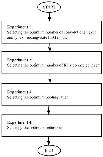
Figure 1.
General methodology used in this paper.
2.3.1. Experiment 1: Selecting the Optimum Number of Convolutional Layers and Type of Resting-State EEG Input
In this experiment, the initial CNN architecture is made up of k convolutional layers (i.e., k is the number of convolutional layers). These k layers are then succeeded by one average pooling layer and one fully connected layer. The number of convolutional layers k is then increased from one layer to twelve layers, each trained and tested using REC, REO, and REC + REO separately, with the mini-batch size and learning rate set at 128 and 0.001, respectively. The optimizer used for the initial CNN architecture was the stochastic gradient descent (SGD). In this experiment, each convolutional layer is made up of six 5 × 5 filters. A filter size of 5 × 5 was selected, as smaller filter sizes such as 3 × 3 can extract features that are too fine, which considered a lower-level feature map. This can result in supplying excessive information to the network and confused the learning progress. On the other hand, large filter sizes such as 7 × 7 can extract feature maps that describe the information too generally. Selecting a moderately sized filter can benefit the feature extraction process. One average pooling layer was placed before the fully connected layer. The smaller filter size of the pooling layer was selected to downsample the resulting feature maps. As the dimension is reduced, the required computational load decreases, resulting in faster processing times. There is a limitation of the resulting feature map that requires features to be extracted at the exact position in the input. Even minor changes in the position of the features can result in a different feature map, which can cause the learning of the architecture to be ineffective. The pooling layer can overcome this issue by performing downsampling on the feature map, generating a lower resolution version of the feature map while at the same time maintaining an important structural element of the input. Any fine detail that may not be useful can be eliminated in this way.
2.3.2. Experiment 2: Selecting the Optimal Number of Fully Connected Layers
This experiment was conducted using the CNN architecture and dataset with the highest identification accuracy from Experiment 1. Using the CNN architecture with the selected number of convolutional layers and type of resting-state input from Experiment 1, Experiment 2 was conducted to select the most suitable number of fully connected layers. The number of fully connected layers was tested for a range of one to four layers with different numbers of neurons, as shown in Table 2.
Table 2.
Different combinations of FC layers and numbers of neurons.
2.3.3. Experiment 3: Selecting the Optimal Pooling Layer
Using the architecture with the highest identification accuracy from Experiment 2, training and testing were carried out using different numbers of average pooling layers with various placement locations. The size of the filter used in the average pooling layer was . Training and testing were repeated using the max-pooling layer to select the optimal type of pooling layer.
2.3.4. Experiment 4: Selecting the Optimal Optimizer
The optimized CNN architecture from Experiment 3 was used to select the optimizer which performed the best for biometrics applications, with both the stochastic gradient descent (SGD) and Adam optimizers considered.
2.4. Performance Measurements
Identification accuracy in terms of percentage was used to gauge the performance of the proposed CNN. Utilizing a one-versus-all strategy, three-fold cross-validation was used to determine the identification accuracy. Subject 1 was labeled as a positive class, while the rest of the 108 subjects were labeled as a negative class. The average of the three-fold cross-validation was recorded. The identification accuracy was calculated as follows:
where is a positive class that is predicted correctly, is a negative class that is identified correctly, is a negative class that is identified wrongly, and is a positive class that is identified wrongly. Identification accuracy was obtained using the testing set. Each of training was repeated five times and the average was obtained.
3. Results and Discussions
This section is divided into six subsections. First, Section 3.1 presents the results of Experiment 1. Next, Section 3.2 provides the results of Experiment 2. The results of Experiment 3 are presented in Section 3.3, and the results from Experiment 4 are provided in Section 3.4. Section 3.5 describes the final CNN architecture, and Section 3.6 compares the performance of the proposed CNN architecture with related works.
3.1. Selection of the Optimal Number of Convolutional Layers and Type of Resting-State EEG Input
The convolutional layer is the key feature that determines the performance of any CNN architecture. It extracts important features that provide information during the training process. The number of convolutional layers affects the output feature maps that are passed into the fully connected layer. Therefore, the number of convolutional layers has to be carefully selected in order to ensure effective feature extraction without losing any information that is critical to obtaining a good identification result. Training and testing were carried out using REC, REO, and REC + REO separately with different numbers of convolutional layers. The convolutional layers (Conv) used in this experiment were made up of six filters with a kernel size of 5 × 5. One average pooling layer (avgpool) with a filter size of was placed before a fully connected layer (FC) with 109 neurons.
The summary of this experiment is presented in Table 3. The highest identification accuracy is in bold, which is the 8 conv + 1 avg pool + 1 FC architecture with eight convolutional layers using the REO dataset. The eighth convolutional layer extracted a 32 × 138 × 6 feature map, which contains the most information from the input. From the results, it can be seen that the REO dataset presents higher identification accuracy in all CNN architectures, suggesting that REO EEG signals are more efficient in discriminating between individuals. Furthermore, the results suggest that there is no proportional relationship between the number of convolutional layers used and the identification accuracy.
Table 3.
Experiment 1: Identification accuracy for CNN architecture with different number of convolutional layers (average ± standard deviation of three-fold cross validation) (%).
3.2. Selection of the Optimal Number of Fully Connected Layers
The fully connected layer in a CNN architecture represents the feed-forward neural network, which plays the role of learning the information from the feature map and classifying each individual’s EEG with the correct label. The fully connected layer initiates the backpropagation learning process of the CNN architecture and confers the most accurate weights. Selecting the optimal number of fully connected layers can affect the learnability of a CNN architecture. The CNN architecture and dataset with the highest identification accuracy in Experiment 1 were used for training and testing using a different number of fully connected layers. The results of Experiment 2 are summarized in Table 4.
Table 4.
Experiment 2: Identification accuracy for CNN architecture with different number of fully connected layers (average ± standard deviation of three-fold cross validation) (%).
It can be seen that the CNN architecture with two FC layers has the highest identification accuracy (), while the CNN architectures with more than two FC layers have degraded identification accuracy. One FC layer is not sufficient for learning from the final feature maps. On the other hand, using a higher number of FC layers increases the architectural complexity and carries the risk of overfitting.
3.3. Selection of the Optimal Number and Type of Pooling Layers
The pooling layer functions to gradually lower the spatial size of the feature map in order to reduce computational complexity. Max pooling and average pooling are the two most widely used types of pooling. Max pooling applies a max-pooling filter to the subregions of the initial representation and obtains the maximum value in the filter region. Average pooling, on the other hand, applies an average filter to obtain the average value in the filter region. In Experiment 3, training and testing were carried out using a different number of average pooling layers, a max-pooling layer, and the placement location of the pooling layer. This experiment was carried out using the CNN architecture previously optimized through Experiments 1 and 2. The results of the experiment using one, two, and three average pooling layers are presented in Table 5, Table 6 and Table 7, respectively.
Table 5.
Experiment 3 (a): Identification accuracy for CNN architecture with one average pooling layer at different locations (average ± standard deviation of three-fold cross validation) (%).
Table 6.
Experiment 3 (b): Identification accuracy for CNN architecture with two average pooling layers at different locations (average ± standard deviation of three-fold cross validation) (%).
Table 7.
Experiment 3 (c): Identification accuracy for CNN architecture with three average pooling layers at different locations (average ± standard deviation of three-fold cross validation) (%).
In this comparison, the CNN architecture with one average pooling layer presented the highest identification accuracy (). Using more than one average pooling layer can cause too much information loss due to the downsizing of the feature map. The results of this experiment suggest that placing one average pooling layer before the fully connected layer can effectively discretize the feature map while retaining important information before passing it to the fully connected layer.
The training and testing processes were repeated using a max-pooling layer, with the results summarized in Table 8, Table 9 and Table 10, respectively. The results for the CNN architecture using a max-pooling layer follow the trend of the average pooling results. However, the max-pooling layer presents slightly lower identification results. This is because average pooling includes all features in the count and then propagates it to the next layer. All information from the previous feature map can then be used for feature mapping and creating an informative output, which is a very generalized computation. In comparison, max-pooling extracts only extreme values, which can cause information loss in the pooling process.
Table 8.
Experiment 3 (d): Identification accuracy for CNN architecture with one max-pooling layer at different locations (average ± standard deviation of three-fold cross validation) (%).
Table 9.
Experiment 3 (e): Identification accuracy for CNN architecture with two max-pooling layers at different locations (average ± standard deviation of three-fold cross validation) (%).
Table 10.
Experiment 3 (f): Identification accuracy for CNN architecture with three max-pooling layers at different locations (average ± standard deviation of three-fold cross validation) (%).
3.4. Selection of the Optimal Optimizer
An optimizer plays an important role in minimizing the training error rate and ensuring that the CNN architecture converges efficiently. To select the most suitable optimizer for our application, SGD and Adam were compared using the architecture from Experiment 3. SGD and Adam were selected for comparison because both are among the most popular and commonly used optimizers. SGD is the most commonly used optimizer; it uses gradient descent to update the weights and bias in the network via backpropagation. On the other hand, the Adam otimizer uses gradient-based optimization of stochastic objective functions, combining the benefits of two SGD advancements: Adaptive Gradient Algorithm (AdaGrad) and Root Mean Square Propagation (RMSProp). It can compute unique adaptive learning degrees for various parameters. At the same time, Adam inherits the advantages of SGD in that direction towards local minima can be determined by relying on the momentum.
The results of this experiment are presented in Table 11. The results indicate that the CNN implementing Adam has higher identification accuracy (). The Adam optimizer presents a lower standard deviation, indicating the training of the CNN architecture with Adam optimizer has more consistent identification accuracy. According to these experimental findings, the advantages of the Adam optimizer are helpful in facilitating effective learning. The design demonstrates improved performance and smoothly converges to the local minima. The learning of the architecture was improved for this investigation by computing a specific learning rate for each weight and bias. The Adam optimizer was therefore chosen as the best optimizer for the suggested architecture.
Table 11.
Experiment 4: Identification accuracy for CNN architecture with different optimizers (average ± standard deviation of three-fold cross validation) (%).
3.5. Proposed Convolutional Neural Network Architecture
Referring to the experimental results, a deep CNN with eleven layers is proposed. The literature shows that most related works have used shallower CNN architectures. A shallow CNN architecture can cause information loss, as the feature maps that are extracted at the convolutional layers are not fine enough. Furthermore, several related works do not implement batch normalization in their work, even though studies have proven that batch normalization is crucial in improving the performance of CNN [44]. In our proposed method, batch normalization is included in the design, and is placed after each convolutional layer. The final CNN architecture used in this study is shown in Table 12, following the architecture’s sequence. There are a total of eleven layers, consisting of eight convolutional layers, one average pooling layer, and two fully connected layers.
Table 12.
Proposed CNN layers and kernel sizes.
For this study, the input to the CNN is a 64 × 160 matrix. The convolutional layers used in this study are made up of six 5 × 5 filters. This small filter size was chosen to extract more precise information and orientation from the signal. The input is passed into the first convolutional layer, creating a 60 × 156 × 6 feature map. For each convolutional layer, rectified linear units (ReLu) are used as the activation function thanks to their sparsity and the reduced likelihood of vanishing gradient. The ReLU function’s primary advantage over other activation functions is that it does not simultaneously fire all of the neurons. The corresponding neuron is not triggered for the negative input values. Compared to the sigmoid and tanh functions, the ReLU function is significantly more computationally efficient, as only a small subset of neurons are active [24].
The resulting feature map proceeds through the second convolutional layer, and a feature map of 56 × 152 × 6 is generated. Then, the feature map is input to the third convolutional layer, generating a feature map of size 52 × 148 × 6. The resulting output is passed to the fourth convolutional layer, outputting a feature map of size 48 × 144 × 6. The fifth convolutional layer creates a feature map of 44 × 140 × 6. The sixth convolutional layer outputs a feature map of size 40 × 136 × 6. After passing the resulting feature map to the seventh convolutional layer, the feature map size is 36 × 132 × 6. The eighth convolutional layer outputs a feature map with size 32 × 128 × 6, and the feature map is passed to the average pooling layer, creating an output of 16 × 64 × 6. After being flattened, the output is subsequently sent to the fully connected layer. The fully connected layers use the softmax activation function, as it can calculate the probability for each class in order to address any classification issues. The feature map output of each hidden layer is summarized in Table 13.
Table 13.
Size of output feature map of each hidden layer.
Seven parameters are fixed, as shown in Table 14. The learning rate is fixed at 0.001 and stays that way during CNN trained. After each convolutional layer, batch normalisation is carried out using the normalisation method. Every training iteration’s mini-batch size is limited to 128. A single epoch that is channelled through the CNN requires 36 iterations, as one epoch has 4578 training subsets. The number of training iterations for each epoch is set at 30, which is a moderate value. This setting was chosen to prevent the network from having an excessively high number of iterations. On the other hand, too few iterations can result in an underfitting of the network with training data, as the repetitions for the training are insufficient. In this experiment, regularization was employed with a regularization factor of 0.0005 to prevent overfitting. The Adam optimizer was been selected for back-propagation during training of the CNN. The Glorot initializer [45], sometimes referred to as the Xavier initializer, was used to pre-define the weights of the suggested architecture. This initializer randomly selects samples from uniformly distributed data with zero mean and variance.
Table 14.
Parameters and values.
3.6. Comparison of the Proposed CNN Architecture with State-of-Art CNNs
Our proposed CNN architecture is compared to the existing CNN-based EEG biometrics identification application in Table 15. By referring to Table 1, it can be seen that our eleven-layer CNN architecture is deeper in comparison to the others. In Table 15, it can be seen that our proposed architecture presents higher identification accuracy than all of the other works except for that of Gui et al. [32] and Wang et al. [38]. In comparison with the work by Gui et al. [32], despite using a shallower architecture, their work manages to present a higher identification accuracy. For their work, active-paradigm EEG signals were used. Using active-paradigm EEG signals presents an advantage compared to task-free paradigms in that discriminating features can be detected. Stimulations or tasks performed at certain time points can become a useful marker to facilitate feature extraction by the convolutional layer. However, active paradigms require longer set up, and may not be applicable for individuals who have lost their cognitive ability.
Table 15.
Performance comparison of the proposed method with other CNN-based EEG biometrics.
In comparison to the work of Wang et al. [38], they used a variety of EEG input types and implemented the input using a combination of active paradigms and task-free paradigms. Such implementation inherits the advantages of both active and task-free paradigm EEG signals. Our proposed method uses only REO EEG as input. By tolerating a slight loss of identification accuracy, our proposed CNN architecture can present high-speed identification, as the subject is only required to open their eyes.
Furthermore, in the exploration of the most suitable type of pooling layer, it can be observed that all of the active paradigms implemented max pooling and obtained high identification accuracy. However, it was found that max pooling does not perform well with task-free paradigms. The purpose of max pooling is to obtain extreme values as features from the input EEG signals, which can be found in active-paradigm EEG when subjects are exposed to external stimulation or are required to perform tasks. Peaks or changes in the signals can be extracted efficiently using max pooling. On the other hand, our experiment shows that average pooling works better with task-free paradigm signals. Average pooling pools the features together by obtaining the average value, which includes all of the data. Therefore, there is no information lost in the process. Ma et al. [28] implemented average pooling in their work as well; however, their work presented a lower identification accuracy due to a shallower CNN architecture, causing the final feature maps to be insufficiently fine.
For additional comparison, the type of activation function and optimizer are tabulated in Table 15, despite there being works that did not mention the type of activation function and optimizer used. All of these works used ReLu as the activation function, again indicating the advantages of ReLu. For the type of optimizer, it can be seen that Adam and SGD were the most commonly used. Therefore, it was worthwhile for us to conduct experiments on SGD and Adam in order to determine which was the best optimizer for our proposed architecture.
Overall, our proposed architecture contains eleven layers, which is deeper than in any of the existing works. As a suitable number of convolutional layers were selected, it is apparent that a deeper CNN architecture can extract an informative feature map, thereby improving identification accuracy. Although a shallow CNN architecture is less complex, a lower number of convolutional layers are insufficient to extract important features from task-free paradigm EEG signals. Moreover, the comparison indicates that average pooling is more suitable for use with task-free paradigm signals, while max pooling is better suited to active-paradigm signals.
4. Conclusions
From our comparison of existing methods with the architecture proposed in this paper, it is clear that the proposed method presents high identification accuracy. The four types of experiments we conducted effectively facilitated the design of a novel deep CNN architecture. In this study, the deep CNN architecture accomplished the feature extraction task adequately using an optimized number of convolutional layers, average pooling layers, fully connected layers, and suitable optimizers. Hence, the proposed architecture presents high identification accuracy and has potential for use in biometrics for safer access to sensitive information and assets.
In the future, other EEG classification strategies can be studied for biometrics applications. Approaches in other areas, such as classification of EEG signals for medical diagnosis [46,47], can be considered as well. In addition to deep learning approaches, fuzzy classification-based approaches such as [48] are worth investigating.
Author Contributions
Conceptualization, S.A.S., M.Z.A. and C.Q.L.; methodology, C.Q.L. and H.I.; software, C.Q.L.; validation, C.Q.L.; formal analysis, C.Q.L. and H.I.; writing—original draft preparation, C.Q.L. and H.I.; writing—review and editing, H.I., M.Z.A. and S.A.S.; supervision, H.I., M.Z.A. and S.A.S.; funding acquisition, H.I. All authors have read and approved the published version of the manuscript.
Funding
The Trans-disciplinary Research Grant Scheme (TRGS) of the Ministry of Higher Education (MoHE), Malaysia, provided funding for this study under grant number TRGS/1/2015/USM/01/6/2.
Data Availability Statement
This work was supported by previously published EEG data, which can be found at https://www.physionet.org/physiobank/database/eegmmidb (accessed on 1 February 2019). At relevant places within the text, this earlier study (and dataset) is cited as reference [40]. In this work, only the REC (i.e., files named as S###R01.edf) and REO (i.e., files named as S###R02.edf) signals were utilized (i.e., ### stands for the volunteer’s index, ranging from 001 to 109).
Acknowledgments
We would like to thank Dato’ Jafri Malin Abdullah, Azlinda Azman, and Aini Ismafairus Abd Hamid for their suggestions regarding our preliminary experiments.
Conflicts of Interest
The authors declare no conflict of interest.
Abbreviations
The following abbreviations are used in this manuscript:
| ANN | Artificial neural network |
| CC | Cross-correlation |
| CNN | Convolutional neural network |
| EEG | Electroencephalography |
| ERP | Event-related potentials |
| FC | Fully connected layer |
| MLP | Multilayer perceptron |
| MoHE | Ministry of Higher Education |
| PSD | Power spectral density |
| REC | Resting-state eyes closed |
| REO | Resting-state eyes open |
| SGD | Stochastic gradient descent |
| SVM | Support vector machine |
| VEP | Visual evoked potentials |
References
- Jain, A.K.; Ross, A.; Prabhakar, S. An introduction to biometric recognition. IEEE Trans. Circuits Syst. Video Technol. 2004, 14, 4–20. [Google Scholar] [CrossRef]
- Revett, K. Cognitive biometrics: A novel approach to continuous person authentication. Int. J. Cogn. Biom. 2012, 1, 1–9. [Google Scholar]
- Lai, C.Q.; Ibrahim, H.; Abdullah, M.Z.; Suandi, S.A. EEG-based biometric close-set identification using CNN-ECOC-SVM. In Artificial Intelligence in Data and Big Data Processing. Lecture Notes on Data Engineering and Communication Technologies, Proceedings of the ICABDE 2021, Ho Chi Minh City, Vietnam, 18–19 December 2021; Dang, N.H.T., Zhang, Y.D., Tavares, J.M.R.S., Chen, B.H., Eds.; Springer: Cham, Switzerland, 2022; Volume 124, p. 124. [Google Scholar]
- Poulos, M.; Rangoussi, M.; Chrissikopoulos, V.; Evangelou, A. Person identification based on parametric processing of the EEG. In Proceedings of the 6th IEEE International Conference on Electronics, Circuits and Systems (Cat. No.99EX357) (ICECS’99), Paphos, Cyprus, 5–8 September 1999; Volume 1, pp. 283–286. [Google Scholar]
- Palaniappan, R.; Mandic, D.P. Biometrics from brain electrical activity: A machine learning approach. IEEE Trans. Pattern Anal. Mach. Intell. 2007, 29, 738–742. [Google Scholar] [CrossRef] [PubMed]
- Marcel, S.; Millan, J.D.R. Person authentication using brainwaves (EEG) and maximum a posteriori model adaptation. IEEE Trans. Pattern Anal. Mach. Intell. 2007, 29, 743–752. [Google Scholar] [CrossRef]
- Campisi, P.; Rocca, D.L. Brain waves for automatic biometric-based user recognition. IEEE Trans. Inf. Forensics Secur. 2014, 9, 782–800. [Google Scholar] [CrossRef]
- Maiorana, E.; Campisi, P. Longitudinal evaluation of EEG-based biometric recognition. IEEE Trans. Inf. Forensics Security 2018, 13, 1123–1138. [Google Scholar] [CrossRef]
- Abo-Zahhad, M.; Ahmed, S.M.; Abbas, S.N. State-of-the-art methods and future perspectives for personal recognition based on electroencephalogram signals. IET Biom. 2015, 4, 179–190. [Google Scholar] [CrossRef]
- Hema, C.R.; Paulraj, M.P.; Kaur, H. Brain signatures: A modality for biometric authentication. In Proceedings of the 2008 International Conference on Electronic Design, Penang, Malaysia, 1–3 December 2008; pp. 1–4. [Google Scholar]
- Ferreira, A.; Almeida, C.; Georgieva, P.; Tomé, A.; Silva, F. Advances in EEG-based biometry. In Image Analysis and Recognition; Campilho, A., Kamel, M., Eds.; Springer: Berlin/Heidelberg, Germany, 2010; pp. 287–295. [Google Scholar]
- Choi, G.; Choi, S.; Hwang, H. Individual identification based on resting-state EEG. In Proceedings of the 2018 6th International Conference on Brain-Computer Interface (BCI), Gangwon, Korea, 15–17 January 2018; pp. 1–4. [Google Scholar]
- Thomas, K.P.; Vinod, A.P. Biometric identification of persons using sample entropy features of EEG during rest state. In Proceedings of the 2016 IEEE International Conference on Systems, Man, and Cybernetics (SMC), Budapest, Hungary, 9–12 October 2016; pp. 003487–003492. [Google Scholar]
- Suppiah, R.; Vinod, A.P. Biometric Identification Using Single Channel EEG during Relaxed Resting State. IET Biom. 2018, 7, 342–348. [Google Scholar] [CrossRef]
- Lee, H.J.; Kim, H.S.; Park, K.S. A study on the reproducibility of biometric authentication based on electroencephalogram (EEG). In Proceedings of the 2013 6th International IEEE/EMBS Conference on Neural Engineering (NER), San Diego, CA, USA, 6–8 November 2013; pp. 13–16. [Google Scholar]
- Fraschini, M.; Hillebrand, A.; Demuru, M.; Didaci, L.; Marcialis, G.L. An eeg-based biometric system using eigenvector centrality in resting state brain networks. IEEE Signal Process. Lett. 2015, 22, 666–670. [Google Scholar] [CrossRef]
- Barry, R.J.; Clarke, A.R.; Johnstone, S.J.; Magee, C.A.; Rushby, J.A. EEG differences between eyes-closed and eyes-open resting conditions. Clin. Neurophysiol. 2007, 118, 2765–2773. [Google Scholar] [CrossRef]
- Travis, T.; Kondo, C.; Knott, J. Parameters of eyes–closed alpha enhancement. Psychophysiology 1974, 11, 674–681. [Google Scholar] [CrossRef] [PubMed]
- Klimesch, W.; Doppelmayr, M.; Pachinger, T.; Russegger, H. Event-related desynchronization in the alpha band and the processing of semantic information. Cogn. Brain Res. 1997, 6, 83–94. [Google Scholar] [CrossRef]
- De Vico Fallani, F.; Vecchiato, G.; Toppi, J.; Astolfi, L.; Babiloni, F. Subject identification through standard eeg signals during resting states. In Proceedings of the 2011 Annual International Conference of the IEEE Engineering in Medicine and Biology Society, Boston, MA, USA, 30 August–3 September 2011; pp. 2331–2333. [Google Scholar]
- Di, Y.; An, X.; He, F.; Liu, S.; Ke, Y.; Ming, D. Robustness analysis of identification using resting-state EEG signals. IEEE Access 2019, 7, 42113–42122. [Google Scholar] [CrossRef]
- Ji, S.; Xu, W.; Yang, M.; Yu, K. 3D convolutional neural networks for human action recognition. IEEE Trans. Pattern Anal. Mach. 2013, 35, 221–231. [Google Scholar] [CrossRef]
- Hinton, G.E.; Salakhutdinov, R.R. Reducing the dimensionality of data with neural networks. Science 2006, 313, 504–507. [Google Scholar] [CrossRef]
- LeCun, Y.; Bengio, Y.; Hinton, G. Deep learning. Nature 2015, 521, 436–444. [Google Scholar] [CrossRef]
- Muhammad, K.; Ahmad, J.; Mehmood, I.; Rho, S.; Baik, S.W. Convolutional neural networks based fire detection in surveillance videos. IEEE Access 2018, 6, 18174–18183. [Google Scholar] [CrossRef]
- Hubel, D.; Wiesel, T. Receptive fields and functional architecture of monkey striate cortex. J. Physiol. 1968, 195, 215–243. [Google Scholar] [CrossRef]
- Lai, C.Q.; Ibrahim, H.; Hamid, A.I.A.; Abdullah, M.Z.; Azman, A.; Abdullah, J.M. Detection of moderate traumatic brain injury from resting-state eye-closed electroencephalography. Comput. Intell. Neurosci. 2020, 2020, 8923906. [Google Scholar] [CrossRef]
- Ma, L.; Minett, J.W.; Blu, T.; Wang, W.S.Y. Resting state EEG-based biometrics for individual identification using convolutional neural networks. In Proceedings of the 2015 37th Annual International Conference of the IEEE Engineering in Medicine and Biology Society (EMBC), Milan, Italy, 25–29 August 2015; pp. 2848–2851. [Google Scholar]
- Sehgal, A.; Kehtarnavaz, N. A convolutional neural network smartphone app for real-time voice activity detection. IEEE Access 2018, 6, 9017–9026. [Google Scholar] [CrossRef]
- Vapnik, V.N. An overview of statistical learning theory. IEEE Trans. Neural Netw. 1999, 10, 988–999. [Google Scholar] [CrossRef] [PubMed]
- Bengio, Y. Learning deep architectures for AI. Found. Trends Mach. Learn. 2009, 2, 1–127. [Google Scholar] [CrossRef]
- Gui, Q.; Yang, W.; Jin, Z.; Ruiz-Blondet, M.V.; Laszlo, S. A residual feature-based replay attack detection approach for brainprint biometric systems. In Proceedings of the 2016 IEEE International Workshop on Information Forensics and Security (WIFS), Abu Dhabi, United Arab Emirates, 4–7 December 2016; pp. 1–6. [Google Scholar]
- Mao, Z.; Yao, W.X.; Huang, Y. EEG-based biometric identification with deep learning. In Proceedings of the 2017 8th International IEEE/EMBS Conference on Neural Engineering (NER), Shanghai, China, 25–28 May 2017; pp. 609–612. [Google Scholar]
- Das, R.; Maiorana, E.; Campisi, P. Visually evoked potential for EEG biometrics using convolutional neural network. In Proceedings of the 2017 25th European Signal Processing Conference (EUSIPCO), Kos, Greece, 28 August–2 September 2017; pp. 951–955. [Google Scholar]
- Schons, T.; Moreira, G.J.P.; Silva, P.H.L.; Coelho, V.N.; Luz, E.J.S. Convolutional network for EEG-based biometric. In Progress in Pattern Recognition, Image Analysis, Computer Vision, and Applications; Mendoza, M., Velastín, S., Eds.; Springer International Publishing: Cham, Switzerland, 2018; pp. 601–608. [Google Scholar]
- El-Fiqi, H.; Wang, M.; Salimi, N.; Kasmarik, K.; Barlow, M.; Abbass, H. Convolution neural networks for person identification and verification using steady state visual evoked potential. In Proceedings of the 2018 IEEE International Conference on Systems, Man, and Cybernetics (SMC), Miyazaki, Japan, 7–10 October 2018; pp. 1062–1069. [Google Scholar]
- Wu, Q.; Zeng, Y.; Zhang, C.; Tong, L.; Yan, B. An EEG-based person authentication system with open-set capability combining eye blinking signals. Sensors 2018, 18, 335. [Google Scholar] [CrossRef] [PubMed]
- Wang, M.; El-Fiqi, H.; Hu, J.; Abbass, H.A. Convolutional neural networks using dynamic functional connectivity for EEG-based person identification in diverse human states. IEEE Trans. Inf. Forensics Secur. 2019, 14, 3259–3272. [Google Scholar] [CrossRef]
- Ozdenizci, O.; Wang, Y.; Koike-Akino, T.; Erdogmus, D. Adversarial deep learning in EEG biometrics. IEEE Signal Process. 2019, 26, 710–714. [Google Scholar] [CrossRef]
- Goldberger, A.L.; Amaral, L.A.N.; Glass, L.; Hausdorff, J.M.; Ivanov, P.C.; Mark, R.G.; Mietus, J.E.; Moody, G.B.; Peng, C.-K.; Stanley, H.E. PhysioBank, PhysioToolkit, and PhysioNet: Components of a new research resource for complex physiologic signals. Circulation 2000, 101, e215–e220. [Google Scholar] [CrossRef]
- Hine, G.E.; Maiorana, E.; Campisi, P. Resting-state EEG: A study on its non-stationarity for biometric applications. In Proceedings of the 2017 International Conference of the Biometrics Special Interest Group (BIOSIG), Darmstadt, Germany, 20–22 September 2017; pp. 1–5. [Google Scholar]
- Lai, C.Q.; Ibrahim, H.; Abdullah, M.Z.; Abdullah, J.M.; Suandi, S.A.; Azman, A. Arrangements of resting state electroencephalography as the input to convolutional neural network for biometric identification. Comput. Intell. Neurosci. 2019, 2019, 7895924. [Google Scholar] [CrossRef]
- Lai, C.Q.; Ibrahim, H.; Hamid, A.I.A.; Abdullah, J.M. LSTM network as a screening tool to detect moderate traumatic brain injury from resting state electroencephalogram. Expert Syst. Appl. 2022, 198, 116761. [Google Scholar] [CrossRef]
- LeCun, Y.; Boser, B.; Denker, J.S.; Henderson, D.; Howard, R.E.; Hubbard, W.; Jackel, L.D. Backpropagation applied to handwritten zip code recognition. Neural Comput. 1989, 1, 541–551. [Google Scholar] [CrossRef]
- Glorot, X.; Bengio, Y. Understanding the difficulty of training deep feedforward neural networks. J. Mach. Learn. Res.-Track 2010, 9, 249–256. [Google Scholar]
- Alotaibi, S.M.; Rahman, A.-U.; Basheer, M.I.; Khan, M.A. Ensemble machine learning based identification of pediatric epilepsy. Comput. Mater. Contin. 2021, 68, 149–165. [Google Scholar]
- Sekkal, R.N.; Bereksi-Reguig, F.; Ruiz-Fernandez, D.; Dib, N.; Sekkal, N. Automatic sleep stage classification: From classical machine learning methods to deep learning. Biomed. Signal Process. Control 2022, 77, 103751. [Google Scholar] [CrossRef]
- Rabcan, J.; Levashenko, V.; Zaitseva, E.; Kvassay, M. Review of methods for EEG signal classification and development of new fuzzy classification-based approach. IEEE Access 2020, 8, 189720–189734. [Google Scholar] [CrossRef]
Publisher’s Note: MDPI stays neutral with regard to jurisdictional claims in published maps and institutional affiliations. |
© 2022 by the authors. Licensee MDPI, Basel, Switzerland. This article is an open access article distributed under the terms and conditions of the Creative Commons Attribution (CC BY) license (https://creativecommons.org/licenses/by/4.0/).