Reliability Estimation of XLindley Constant-Stress Partially Accelerated Life Tests using Progressively Censored Samples

Abstract

It often takes a lot of time to conduct life-testing studies on products or components. Units can be tested under more severe circumstances than usual, known as accelerated life tests, to reduce the testing period. This study’s goal is to look into certain estimation issues related to point and interval estimations for XLindley distribution under constant stress partially accelerated life tests with progressive Type-II censored samples. The maximum likelihood approach is utilized to acquire the point and interval estimates of the model parameters as well as the reliability function under normal use conditions. The Bayesian estimation method using the Monte Carlo Markov Chain procedure using the squared error loss function is also provided. Moreover, the Bayes credible intervals as well as the highest posterior density credible intervals of the different parameters are considered. To make comparisons between the proposed methods, a simulation study is conducted with various sample sizes and different censoring schemes. The usefulness of the suggested methodologies is then demonstrated by the analysis of two data sets. A summary of the major findings of the study can be found in the conclusion.

1. Introduction

Life testing under normal use conditions is definitely the most convenient way for determining a product’s quality or comparing various manufacturing designs. A continuous improvement in manufacturing design often leads to products with a significantly longer lifespan and a high degree of reliability. In these circumstances, the conventional life testing techniques may be time-consuming to gather the necessary failure data required to draw the desired inference. In these situations, experimenters conduct the accelerated life tests (ALTs), in which the test units are put under stress conditions that are more severe than usual to ensure rapid failure and minimize the testing period. Although there are various ALT models, the constant-stress and step-stress models are the two that are most commonly utilized. A constant-stress ALT is used when placing each unit under test at continuous stress until the test is complete or all units fail. Conversely, a step-stress ALT gradually raises the stress after a prefixed number of failures or at predetermined times. There are numerous studies that take into account different ALT models: for instance, Mohie El-Din et al. [1], Samanta et al. [2], Wang [3], Cui et al. [4], Nassar et al. [5] and Kumar et al. [6]. The ALTs assume that a product’s lifetime and stress conditions have a known relationship; therefore, data obtained under accelerated settings can rely upon under normal use conditions. The existence of life-stress models is not always known. Consequently, one method of assessing a product’s reliability in conditions of normal use is through a partially accelerated life test (PALT). The constant-stress PALT (CSPALT) is one of the PALT types on which this study focuses. All test unit groups in CSPALT are independently placed in use conditions and accelerated conditions. The test procedure and basic assumptions of CSPALT are discussed in the next section. The CSPALTs have also been considered in numerous studies, for example Hyun and Lee [7], Mohamed [8], Dey et al. [9], Eliwa and Ahmed [10] and Almarashi [11].

Even though the primary goal of the ALTs is to reduce the length of the experiment’s test period, the researchers spend a lot of time waiting for all test units to fail. Dealing with censored data is important for this. In reliability studies and life-testing experiments, censoring is a relatively common scenario. Broadly speaking, censoring indicates that actual failure durations are only known for a part of the study units where the units are withdrawn from the test before failure due to time and expense constraints. In practice, many censoring plans are available including one-stage and multi-stage censoring schemes. One of the most widespread and flexible censoring strategies is the progressive Type-II censoring (PT-IIC) scheme. Consider the PT-IIC scheme in which $(S_1,S_2,\cdots ,S_m)$ is a prefixed censoring plan and n units are subjected to a life test with a predetermined number of failures m. $S_1$ units are at random taken away from the remaining surviving units after the first failure occurs. Similarly, $S_2$ units are randomly removed from the test when the second failure happens, and so on. The test is run until the mth failure; then, all of the remaining units $S_m=n-m-{\sum }_{i=1}^{m-1}{S}_i$ are taken out of the test, and the experiment is over. It should be emphasized that the PT-IIC scheme offers distinct advantages over traditional Type-I and Type-II censoring schemes in that it enables experimenters to remove survival testing units from the experiment at various testing stages. Numerous authors have explored the PT-IIC scheme with various lifetime distributions; see for example Rastogi and Tripathi [12], Sultan et al. [13], Wu and Gui [14], Alotaibi et al. [15] and Bedbur and Mies [16]. One may refer to the in-depth review study by Balakrishnan [17].

The Lindley distribution, which was first postulated by Lindley [18], has been much studied in a variety of scientific and technological fields. For the research of stress-strength reliability modeling, it is a crucial statistical model. Recently, Chouia and Zeghdoudi [19] introduced the XLindley (XL) distribution as a novel modification of the Lindley distribution that combines the exponential and Lindley distributions. Assume that the lifetime random variable Y of the experimental unit follows the XL distribution with scale parameter $\beta$. In light of this, the relevant probability density function (PDF) and cumulative distribution function (CDF) of Y are provided, respectively, by

$$f_1(y;\beta )=\frac{{\beta }^2\left(\beta +y+2\right)}{{\left(1+\beta \right)}^2}{e}^{-\beta y},y>0,\beta >0,$$

(1)

and

$$F_1(y;\beta )=1-e^{-\beta y}\left[1+\frac{\beta y}{{\left(1+\beta \right)}^2}\right].$$

(2)

The ability of a component to perform as planned for a predetermined amount of time is referred to as reliability. The reliability function (RF) and hazard rate function (HRF) are the two reliability indices that are most frequently employed in practice. For the XL distribution, the RF and HRF are given, respectively, as follows

$$R_1(y;\beta )=e^{-\beta y}\left[1+\frac{\beta y}{{\left(1+\beta \right)}^2}\right]$$

(3)

and

$$h_1(y;\beta )=\frac{{\beta }^2\left(\beta +y+2\right)}{{\left(1+\beta \right)}^2+\beta y}.$$

(4)

We are motivated to do this work because of (1) the XL distribution’s flexibility in modelling different kinds of data and (2) the efficiency of integrating CSPALTs with the PT-IIC scheme in shortening the test period and extrapolating the product performance under normal use conditions. Furthermore, there were no studies reported on estimating the XL distribution’s parameters using CSPALTs with PT-IIC samples. Our main objective in this study is to discuss the estimation of the unknown parameter of the XL distribution as well as the acceleration factor under CSPALT with PT-IIC samples. The RF under normal use conditions is also estimated. To achieve this, the maximum likelihood and Bayesian estimation methods are considered. Based on the asymptotic properties of the maximum likelihood estimates (MLEs), two approximate confidence intervals (ACIs) of the unknown parameters are obtained, namely, ACIs using normal approximation (ACI-NA) and ACIs using the normality of the log-transformed MLEs, which is denoted by ACI-NL. The Bayes estimates are obtained through the Monte Carlo Markov Chain (MCMC) procedure using the squared error (SE) loss function. The Bayes credible intervals (BCIs) as well as the highest posterior density (HPD) credible intervals of the unknown parameters are also investigated. A simulation study and two applications are provided to compare the various techniques and show the applicability of the proposed methods.

The remainder of this article is structured as follows: The model description is discussed in Section 2. The MLEs and ACIs for the unknown parameters are established in Section 3. The Bayesian estimation is considered in Section 4. The effectiveness of the suggested methods is investigated through an extensive simulation study in Section 5. Two applications are presented in Section 6. Finally, Section 7 provides some concluding observations.

2. Model Description

The following is a description of the CSPALT procedure which uses the PT-IIC samples along with its underlying assumptions.

2.1. Testing Procedure

In a CSPALT in the presence of PT-IIC samples, we have the following:

• The experimenter divides the n test products into two sets: The first set contains $n_1$ products that are randomly picked from the n test products and placed in normal operating conditions. The second set contains $n_2=n-n_1$ remaining products that are placed in an accelerated situation.
• Let $n_k,k=1,2$ denote the number of products tested using PT-IIC with progressive censoring plans $S_{k1},S_{k2},\cdots ,S_{k{m}_k}$ under normal and accelerated conditions, respectively, and $m_k,k=1,2$ denote the number of failures actually observed under normal and accelerated configurations, respectively. In this case, one can observe the following example

  $$y_{k1:m_k:n_k}<y_{k2:m_k:n_k}<\cdots <y_{k{m}_k:m_k:n_k},k=1,2.$$

2.2. Basic Assumptions

The following assumptions are required to allow us to deal with CSPALT:

• The lifetime of the product under normal use follows the XL distribution, with PDF, CDF, SF, and HRF as specified in (1)–(4).
• The HRF of a product working under accelerated conditions is determined by the following formula

  $$h_2(y;\beta )=\delta h_1(y;\beta ),$$

  where $h_1(y;\beta )$ is specified by (4) and $\delta >1$ is an acceleration factor.

With the help of the aforementioned assumptions, the HRF under the accelerated condition can be derived as shown below

$$\begin{array}{c}\hfill h_2(y;\beta ,\delta )=\frac{\delta {\beta }^2\left(\beta +y+2\right)}{{\left(1+\beta \right)}^2+\beta y}.\end{array}$$

(5)

Making use of the link $R_2(y;\beta ,\delta )=exp\left[-{\int }_0^y{h}_2(x;\beta ,\delta )dx\right]$, the RF can be acquired under the accelerated condition as

$$R_2(y;\beta ,\delta )=e^{-\beta \delta y}{\left[1+\frac{\beta y}{{\left(1+\beta \right)}^2}\right]}^{\delta }.$$

(6)

The PDF and CDF corresponding to (6) are given, respectively, by

$$f_2(y;\beta ,\delta )=\frac{\delta {\beta }^2\left(\beta +x+2\right)}{{(1+\beta )}^2}{e}^{-\beta \delta y}{\left[1+\frac{\beta y}{{\left(1+\beta \right)}^2}\right]}^{\delta -1}$$

(7)

and

$$F_2(y;\beta ,\delta )=1-e^{-\beta \delta y}{\left[1+\frac{\beta y}{{\left(1+\beta \right)}^2}\right]}^{\delta }.$$

(8)

The joint likelihood function, devoid of the constant term, can be defined as follows based on the realizations of the two PT-IIC samples with CSPALT

$$L(\beta ,\delta |\mathit{y})=\prod _{k=1}^2\left\{\prod _{i=1}^{m_k}{f}_k\left(y_{ki}\right){[1-F_k\left(y_{ki}\right)]}^{S_{ki}}\right\},$$

(9)

where $y_{ki}=y_{ki:m_k:n_k}$ for simplicity and $\mathit{y}=(y_{k1},\cdots ,y_{k{m}_k}),k=1,2$.

3. Maximum Likelihood Estimation

The point and interval estimations of the unknown parameters $\beta$ and $\delta$ based on the PT-IIC sample with CSPALT are obtained in this part using the maximum likelihood approach. In addition, we obtain the MLE and ACI of the RF under normal use conditions. Let $Y_{11}<Y_{12}<\dots <Y_{1m_1}$ be a PT-IIC sample with progressive censoring plan $(S_{11},S_{12},\cdots ,S_{1m_1})$ selected from the XL population at normal use conditions with PDF and CDF given by (1) and (2), respectively. On the other hand, suppose that $Y_{21}<Y_{22}<\dots <Y_{2m_2}$ is a PT-IIC sample with progressive censoring scheme $(S_{21},S_{22},\cdots ,S_{2m_2})$ picked from the XL population at accelerated condition with PDF and CDF provided by (7) and (8), respectively. The likelihood function of the observed samples can then be written as follows from (9)

$$\begin{array}{ccc}\hfill L(\beta ,\delta |\mathit{y})& =& \frac{{\delta }^{m_2}{\beta }^{2m}}{{(1+\beta )}^{2m}}exp\left[-\beta \sum _{k=1}^2\sum _{i=1}^{m_k}{\delta }^{k-1}{Q}_{ki}{y}_{ki}+\sum _{k=1}^2\sum _{i=1}^{m_k}log(\beta +y_{ki}+2)\right]\hfill \\ & \times & \prod _{k=1}^2\prod _{i=1}^{m_k}{\left[1+\frac{\beta y_{ki}}{{\left(1+\beta \right)}^2}\right]}^{{\delta }^{k-1}{Q}_{ki}-1},\hfill \end{array}$$

(10)

where $m=m_1+m_2$ and $Q_{ki}=1+S_{ki}$. The natural logarithm corresponding to (10), denoted by $\ell (\beta ,\delta |\mathit{y})$, can be written as

$$\begin{array}{ccc}\hfill \ell (\beta ,\delta |\mathit{y})& =& m_{2}log\left(\delta \right)+2mlog\left(\beta \right)-2mlog(\beta +1)-\beta \sum _{k=1}^2\sum _{i=1}^{m_k}{\delta }^{k-1}{Q}_{ki}{y}_{ki}\hfill \\ & +& \sum _{k=1}^2\sum _{i=1}^{m_k}log(\beta +y_{ki}+2)+\sum _{k=1}^2\sum _{i=1}^{m_k}({\delta }^{k-1}{Q}_{ki}-1)log\left[1+\frac{\beta y_{ki}}{{\left(1+\beta \right)}^2}\right].\hfill \end{array}$$

(11)

The simultaneous solution of the following normal equations yields the MLEs of $\beta$ and $\delta$, represented by $\widehat{\beta }$ and $\widehat{\delta }$,

$$\begin{array}{ccc}\hfill \frac{\partial \ell (\beta ,\delta |\mathit{y})}{\partial \beta }& =& \frac{2m}{\beta }-\frac{2m}{\beta +1}-\sum _{k=1}^2\sum _{i=1}^{m_k}{\delta }^{k-1}{Q}_{ki}{y}_{ki}+\sum _{k=1}^2\sum _{i=1}^{m_k}\frac{1}{\beta +y_{ki}+2}\hfill \\ & -& \frac{\beta -1}{\beta +1}\sum _{k=1}^2\sum _{i=1}^{m_k}\frac{({\delta }^{k-1}{Q}_{ki}-1)y_{ki}}{1+\beta (\beta +y_{ki}+2)}=0\hfill \end{array}$$

(12)

and

$$\begin{array}{c}\hfill \frac{\partial \ell (\beta ,\delta |\mathit{y})}{\partial \delta }=\frac{m_2}{\delta }-\beta \sum _{i=1}^{m_2}{Q}_{2i}{y}_{2i}+\sum _{i=1}^{m_2}{Q}_{2i}log\left[1+\frac{\beta y_{2i}}{{\left(1+\beta \right)}^2}\right]=0.\end{array}$$

(13)

Using (13) and for fixed $\beta$, one can obtain the MLE of the unknown parameter $\delta$ as a function of the parameter $\beta$ as shown below

$$\begin{array}{ccc}\hfill \widehat{\delta }\left(\beta \right)& =& \frac{m_2}{\beta {\sum }_{i=1}^{m_2}{Q}_{2i}{y}_{2i}-{\sum }_{i=1}^{m_2}{Q}_{2i}log\left[1+\frac{\beta y_{2i}}{{\left(1+\beta \right)}^2}\right]}.\hfill \end{array}$$

(14)

By substituting $\widehat{\delta }\left(\beta \right)$ in the normal equation given by (12), the MLE of $\beta$ can be obtained by solving the following non-linear equation

$$\begin{array}{ccc}\hfill \frac{\partial \ell (\beta ,\delta |\mathit{y})}{\partial \beta }& =& \frac{2m}{\beta }-\frac{2m}{\beta +1}-\sum _{k=1}^2\sum _{i=1}^{m_k}{\left[\widehat{\delta }\left(\beta \right)\right]}^{k-1}{Q}_{ki}{y}_{ki}+\sum _{k=1}^2\sum _{i=1}^{m_k}\frac{1}{\beta +y_{ki}+2}\hfill \\ & -& \frac{\beta -1}{\beta +1}\sum _{k=1}^2\sum _{i=1}^{m_k}\frac{({\left[\widehat{\delta }\left(\beta \right)\right]}^{k-1}{Q}_{ki}-1)y_{ki}}{1+\beta (\beta +y_{ki}+2)}=0\hfill \end{array}$$

(15)

It is worth highlighting that Equation (15) is analytically impossible to solve. Therefore, acquiring the MLE $\widehat{\beta }$ in explicit form is challenging. The requisite estimate can be obtained using some numerical approaches, such as the Newton–Raphson method. Another approach to obtain the MLE of $\beta$ is to use the iterative process as mentioned by Pareek et al. [20]. Since the profile log-likelihood function of $\beta$ is unimodal as displayed in Figure 1, we can write $h\left(\beta \right)=\beta$, where

$$\begin{array}{ccc}\hfill h\left(\beta \right)& =& \frac{2m}{\frac{2m}{\beta +1}+{\sum }_{k=1}^2{\sum }_{i=1}^{m_k}{\left[\widehat{\delta }\left(\beta \right)\right]}^{k-1}{Q}_{ki}{y}_{ki}-{\sum }_{k=1}^2{\sum }_{i=1}^{m_k}\frac{1}{\beta +y_{ki}+2}+\frac{\beta -1}{\beta +1}{\sum }_{k=1}^2{\sum }_{i=1}^{m_k}\frac{({\left[\widehat{\delta }\left(\beta \right)\right]}^{k-1}{Q}_{ki}-1)y_{ki}}{1+\beta (\beta +y_{ki}+2)}}.\hfill \end{array}$$

(16)

Then, the MLE of $\beta$ can be acquired by performing the following steps:

Step 1.

Set the initial value of $\beta$, say ${\beta }^{\left(0\right)}$.

Step 2.

Put $k=1$.

Step 3.

Compute ${\beta }^{\left(k\right)}=h\left({\beta }^{(k-1)}\right)$.

Step 4.

Proceed in this way to obtain ${\beta }^{(k+1)}=h\left({\beta }^{\left(k\right)}\right)$.

Step 5.

Stop the iteration at $|{\beta }^{(k+1)}-{\beta }^{\left(k\right)}|<\varsigma$, where $\varsigma$ is a pre-assigned tolerance bound.

Step 6.

Put $\widehat{\beta }={\beta }^{(k+1)}$.

After obtaining the MLE $\widehat{\beta }$, the MLE $\widehat{\delta }=\widehat{\delta }\left(\beta \right)$ can be determined from (14) by replacing $\beta$ by its MLE. Using the MLEs’ invariance property, it is possible to obtain from (3) the MLE of the RF under normal operating conditions at time t, indicated by ${\widehat{R}}_1\left(t\right)$, as shown below

$${\widehat{R}}_1\left(t\right)=e^{-\widehat{\beta }t}\left[1+\frac{\widehat{\beta }t}{{\left(1+\widehat{\beta }\right)}^2}\right].$$

(17)

It is observed from (14) that $\widehat{\delta }$ can be obtained in an explicit form as a function of the MLE of the parameter $\beta$. As a result, the MLE of $\delta$ exists and is unique if the MLE of $\beta$ exists and is unique. In our case, it is not easy to show the existence and uniqueness of $\beta$ due to the complicated expression of its normal equation. To overcome this difficulty, we try to prove these properties numerically by simulating two PT-IIC samples with progressive censoring plan $S_{ki}=(1^{19},11),k=1,2,i=1,\cdots ,20$ and $1^{19}$ means that 1 is repeated 19 times, using $\beta =3$ and $\delta =2$. The MLEs of $\beta$ and $\delta$ are 2.925011 and 1.816687, respectively. For fixed $\widehat{\delta }=1.816687$, the log-likelihood function given by (11) and the normal equation of $\beta$ given by (12) are drawn for a given sequence of $\beta$; see Figure 1. It shows that the vertical line which is the MLE of $\beta$ intersects the log-likelihood curve at its peak and intersects with the first derivative at zero. Consequently, one can conclude that the ML of the parameter $\beta$ exists and is unique.

It is particularly hard to identify the exact distributions of the MLEs because they do not exist in closed form. Accordingly, based on the asymptotic normality of the MLEs which essentially implies that as the sample size increases, the MLEs estimators are asymptotically distributed with Gaussian behavior, we propose utilizing the ACIs of the unknown parameters $\beta$ and $\delta$ as well as the RF under normal operating conditions. The observed Fisher information matrix is needed for this procedure, where its inverse is the asymptotic variance–covariance matrix, denoted by ${\mathit{I}}^{-1}(\widehat{\beta },\widehat{\delta })$, and given as follows

$$\begin{array}{c}\hfill {\mathit{I}}^{-1}(\widehat{\beta },\widehat{\delta })={\left(\begin{array}{cc}-\frac{{\partial }^2\ell (\beta ,\delta |\mathit{y})}{\partial {\beta }^2}& -\frac{{\partial }^2\ell (\beta ,\delta |\mathit{y})}{\partial \beta \partial \delta }\\ -\frac{{\partial }^2\ell (\beta ,\delta |\mathit{y})}{\partial \delta \partial \beta }& -\frac{{\partial }^2\ell (\beta ,\delta |\mathit{y})}{\partial {\delta }^2}\end{array}\right)}_{\beta =\widehat{\beta },\delta =\widehat{\delta }}^{-1}=\left(\begin{array}{cc}{\widehat{\sigma }}_{11}^2& {\widehat{\sigma }}_{12}\\ & {\widehat{\sigma }}_{22}^2\end{array}\right),\end{array}$$

(18)

where

$$\begin{array}{ccc}\hfill \frac{{\partial }^2\ell (\beta ,\delta |\mathit{y})}{\partial {\beta }^2}& =& -\frac{2m}{{\beta }^2}+\frac{2m}{{(\beta +1)}^2}-\sum _{k=1}^2\sum _{i=1}^{m_k}\frac{1}{{(\beta +y_{ki}+2)}^2}\hfill \\ & -& \frac{1}{{(\beta +1)}^2}\sum _{k=1}^2\sum _{i=1}^{m_k}\frac{({\delta }^{k-1}{Q}_{ki}-1)y_{ki}[4+y_{ki}+\beta (2y_{ki}-\beta y_{ki}-2{\beta }^2+6)]}{{[1+\beta (\beta +y_{ki}+2)]}^2},\hfill \end{array}$$

$$\begin{array}{c}\hfill \frac{{\partial }^2\ell (\beta ,\delta |\mathit{y})}{\partial {\delta }^2}=-\frac{m_2}{{\delta }^2}\end{array}$$

and

$$\begin{array}{ccc}\hfill \frac{{\partial }^2\ell (\beta ,\delta |\mathit{y})}{\partial \beta \partial \delta }& =& -\sum _{i=1}^{m_2}{Q}_{2i}{y}_{2i}-\frac{\beta -1}{\beta +1}\sum _{i=1}^{m_2}\frac{Q_{2i}{y}_{2i}}{1+\beta (\beta +y_{2i}+2)}.\hfill \end{array}$$

As a result, the $100(1-ϵ)\%$ ACIs-NA of $\beta$ and $\delta$ can be computed, respectively, as

$$\widehat{\beta }\pm z_{ϵ/2}{\widehat{\sigma }}_{11},\mathrm{and}\widehat{\delta }\pm z_{ϵ/2}{\widehat{\sigma }}_{22},$$

where $z_{ϵ/2}$ is the upper $(ϵ/2)$th percentile point of the standard normal distribution. On the other hand, building the RF’s ACI-NA at normal use conditions is essential. In this situation, we need first to determine the variance of its estimator $\widehat{R}\left(t\right)$. In this scenario, we consider approximating the necessary variance using the delta approach. According to the delta method, if the random variable is asymptotically normal, we can reasonably approximate the asymptotic behavior of any function over it. Following this approach, the estimated variance of $\widehat{R}\left(t\right)$ can be approximated as ${\widehat{\sigma }}_R^2=[\Delta {\mathit{I}}^{-1}(\widehat{\beta },\widehat{\delta }){\Delta }^{\top }]$, with $\Delta =\left(d{R}_1\left(t\right)/\partial \beta ,0\right){|}_{\beta =\widehat{\beta }}$, where

$$\frac{d{R}_1\left(t\right)}{\partial \beta }=\frac{t\beta e^{-\beta t}[4+t+\beta (3+t+\beta )]}{{(1+\beta )}^3}.$$

Now, the $100(1-ϵ)$ ACI-NA for $R_1\left(t\right)$ is

$${\widehat{R}}_1\left(t\right)\pm z_{ϵ/2}{\widehat{\sigma }}_R.$$

There are some drawbacks to the ACIs-NA discussed above. When the sample size is small, for example, they give a low coverage probability. For positive parameters, it occasionally provides negative lower bounds; see for more detail Maiti et al. [21]. To improve on the unsatisfactory performance of the ACIs-NA, we can use the normal approximation of the log-transformed MLEs to obtain the $100(1-ϵ)$ ACIs-NL of $\beta ,\delta$ and $R_1\left(t\right)$ as follows

$$\widehat{\beta }exp\left[\pm \frac{z_{ϵ/2}{\widehat{\sigma }}_{11}}{\widehat{\beta }}\right],\widehat{\delta }exp\left[\pm \frac{z_{ϵ/2}{\widehat{\sigma }}_{22}}{\widehat{\delta }}\right]\mathrm{and}{\widehat{R}}_1\left(t\right)exp\left[\pm \frac{z_{ϵ/2}{\widehat{\sigma }}_R}{{\widehat{R}}_1\left(t\right)}\right].$$

4. Bayesian Estimation

The Bayesian estimation of the unknown parameters $\beta$ and $\delta$ as well as the RF under normal use settings are the key topic of this section. It should be mentioned that the loss functions and prior distributions are crucial when studying estimation problems from a Bayesian perspective. The symmetric SE loss function is used in our analysis, but the findings can be applied to any other loss function as well. Following the same approach by Nassar and Elshahhat [22], we consider that the two parameters are independent, where the random variable $\beta$ follows the gamma distribution (G), i.e., $\beta \sim G(a_1,b_1)$. On the other hand, the random variable $\delta$ is assumed to follow the three-parameter G distribution with a location parameter equal to one, i.e., $\delta \sim G(a_2,b_2,1)$. Utilizing these assumptions, we can formulate the joint prior distribution of $\beta$ and $\delta$ as follows

$$\pi (\beta ,\delta )\propto {\beta }^{a_1-1}{(\delta -1)}^{a_2-1}{e}^{-[b_1\beta +b_2(\delta -1)]},\beta >0,\delta >1,$$

(19)

where $a_j>0$ and $b_j>0,j=1,2$ are the hyper-parameters. The joint posterior distribution of $\beta$ and $\delta$ can be expressed by combining the likelihood function provided by (10) with the joint prior distribution as shown in (19) as

$$\begin{array}{ccc}\hfill g(\beta ,\delta |\mathit{y})& =& \frac{{\beta }^{2m+a_1-1}}{A{(1+\beta )}^{2m}}exp\left\{-\beta \left[\sum _{k=1}^2\sum _{i=1}^{m_k}{(\delta -1)}^{k-1}{Q}_{ki}{y}_{ki}+b_1\right]+\sum _{k=1}^2\sum _{i=1}^{m_k}log(\beta +y_{ki}+2)\right\}\hfill \\ & \times & {(\delta -1)}^{m_2+a_2-1}{e}^{-b_2(\delta -1)}\prod _{k=1}^2\prod _{i=1}^{m_k}{\left[1+\frac{\beta y_{ki}}{{\left(1+\beta \right)}^2}\right]}^{{(\delta -1)}^{k-1}{Q}_{ki}-1},\hfill \end{array}$$

(20)

where A stands for the normalized constant and is defined as

$$\begin{array}{c}\hfill A={\int }_1^{\infty }{\int }_0^{\infty }L(\beta ,\delta |\mathit{y})\pi (\beta ,\delta )d\beta d\delta .\end{array}$$

In light of this, the Bayes estimate of any function of $\beta$ and $\delta$, say $\psi (\beta ,\delta )$, under SE loss function can be obtained directly from the posterior distribution in (20) as follows

$$\begin{array}{ccc}\hfill \tilde{\psi }(\beta ,\delta )& =& E_{\beta ,\delta |\mathit{y}}\left[\psi (\beta ,\delta )\right]\hfill \\ & =& {\int }_1^{\infty }{\int }_0^{\infty }\psi (\beta ,\delta )g(\beta ,\delta |\mathit{y})d\beta d\delta \hfill \end{array}$$

(21)

It is clear that for general $\psi (\beta ,\delta )$, an analytical evaluation of (21) will not be possible. We propose to directly produce samples from the joint posterior distribution in (20) using the MCMC approach, and then, using the samples that were generated, we present a simulation-consistent estimate of (21) along with the related BCI and HPD interval. It is necessary to determine the full conditional distributions of $\beta$ and $\delta$ in order to use the MCMC process. For $\beta$ and $\delta$, respectively, the necessary conditional distributions can be constructed from (20) as follows

$$\begin{array}{ccc}\hfill g\left(\beta \right|\delta ,\mathit{y})& \propto & \frac{{\beta }^{2m+a_1-1}}{{(1+\beta )}^{2m}}exp\left\{-\beta \left[\sum _{k=1}^2\sum _{i=1}^{m_k}{(\delta -1)}^{k-1}{Q}_{ki}{y}_{ki}+b_1\right]+\sum _{k=1}^2\sum _{i=1}^{m_k}log(\beta +y_{ki}+2)\right\}\hfill \\ & \times & \prod _{k=1}^2\prod _{i=1}^{m_k}{\left[1+\frac{\beta y_{ki}}{{\left(1+\beta \right)}^2}\right]}^{{(\delta -1)}^{k-1}{Q}_{ki}-1},\hfill \end{array}$$

(22)

and

$$\begin{array}{ccc}\hfill g\left(\delta \right|\beta ,\mathit{y})& =& {(\delta -1)}^{m_2+a_2-1}exp\left\{-(\delta -1)\left[\beta \sum _{i=1}^{m_2}{Q}_{2i}{y}_{2i}-\sum _{i=1}^{m_2}{Q}_{2i}log\left[1+\frac{\beta y_{2i}}{{\left(1+\beta \right)}^2}\right]+b_2\right]\right\}.\hfill \end{array}$$

(23)

Any of the gamma-generating routines can be used to easily create samples of $\delta$ because it is evident that its conditional distribution shown in (23) is a three-parameter G distribution with location parameter equal to one, shape parameter $a^{*}=m_2+a_2$ and scale parameter given by

$$\begin{array}{c}\hfill b^{*}=\beta \sum _{i=1}^{m_2}{Q}_{2i}{y}_{2i}-\sum _{i=1}^{m_2}{Q}_{2i}log\left[1+\frac{\beta y_{2i}}{{\left(1+\beta \right)}^2}\right]+b_2.\end{array}$$

The conditional distribution of the parameter $\beta$, which is provided by Equation (22), on the other hand, is unknown, but its plot shows that it has the same behavior as the normal distribution; see Figure 2. As a result, we consider creating samples from this distribution based on the Metropolis–Hastings (M-H) method.

To obtain samples of $\beta$ and $\delta$, utilize the following M-H-within-Gibbs sampling procedures.

Step 1.

Set $j=1$ and put the initial guesses of $\beta$ and $\delta$ as $({\beta }^{\left(0\right)},{\delta }^{\left(0\right)})=(\widehat{\beta },\widehat{\delta })$.

Step 2.

Generate ${\delta }^{\left(j\right)}$ from $G(a^{*},b^{*},1)$ using ${\beta }^{(j-1)}$.

Step 3.

Generate ${\beta }^{\left(j\right)}$ using the M-H procedure from (22) with $N({\beta }^{(j-1)},{\widehat{\sigma }}_{11})$.

Step 4.

Use ${\delta }^{\left(j\right)}$ and ${\beta }^{\left(j\right)}$ to compute $R_1^{\left(j\right)}\left(t\right)$.

Step 5.

Set $j=j+1$.

Step 6.

Repeat steps 2 to 5, M times to acquire $[{\beta }^{\left(j\right)},{\delta }^{\left(j\right)},R_1^{\left(j\right)}\left(t\right)],j=1,\cdots ,M$.

The first B generated variates are discarded in order to ensure convergence and remove the influence of the choice of beginning values. We currently have $[{\beta }^{\left(j\right)},{\delta }^{\left(j\right)},R_1^{\left(j\right)}\left(t\right)],j=B+1,\cdots ,M$. Based on large M, we can use the created samples to calculate the Bayes estimates, BCIs and HPD credible intervals. Using the SE loss function, the Bayes estimates of $\beta ,\delta$ and $R_1\left(t\right)$ are as follows

$$\begin{array}{c}\hfill \tilde{\beta }=\frac{{\sum }_{j=B+1}^M{\beta }^{\left(j\right)}}{M^{*}},\tilde{\delta }=\frac{{\sum }_{j=B+1}^M{\delta }^{\left(j\right)}}{M^{*}}\mathrm{and}{\tilde{R}}_1\left(t\right)=\frac{{\sum }_{j=B+1}^M{R}_1^{\left(j\right)}\left(t\right)}{M^{*}},\end{array}$$

where $M^{*}=M-B$. To compute the BCIs or HPD credible intervals, we first order $[{\beta }^{\left(j\right)},{\delta }^{\left(j\right)},R_1^{\left(j\right)}\left(t\right)],j=B+1,\cdots ,M$. Then, the $100(1-ϵ)\%$ BCIs of $\beta ,\delta$ and $R_1\left(t\right)$ can be determined as shown below

$$\begin{array}{c}\hfill \left[{\beta }^{\left(L^{*}\right)},{\beta }^{\left(U^{*}\right)}\right],\left[{\delta }^{\left(L^{*}\right)},{\delta }^{\left(U^{*}\right)}\right]\mathrm{and}\left[R_1^{\left(L^{*}\right)}\left(t\right),R_1^{\left(U^{*}\right)}\left(t\right)\right],\end{array}$$

where $L^{*}=ϵM^{*}/2$ and $U^{*}=M^{*}(1-ϵ/2)$. On the other hand, the $100(1-ϵ)\%$ two-sided HPD credible intervals of $\beta ,\delta$ and $R_1\left(t\right)$ are given by

$$\begin{array}{c}\hfill \left[{\beta }^{\left(j^{*}\right)},{\beta }^{\left(j^{*}+U^{\star }\right)}\right],\left[{\delta }^{\left(j^{*}\right)},{\delta }^{\left(j^{*}+U^{\star }\right)}\right]\mathrm{and}\left[R_1^{\left(j^{*}\right)}\left(t\right),R_1^{\left(j^{*}+U^{\star }\right)}\left(t\right)\right],\end{array}$$

where $U^{\star }=(1-ϵ)M^{*}$ and $j^{*}=B+1,B+2,\cdots ,M$ is determined, for any parameter say $\lambda$, to satisfy

$${\lambda }^{\left(j^{*}+\left[U^{\star }\right]\right)}-{\lambda }^{\left(j^{*}\right)}=\underset{1⩽j⩽ϵ\left(M^{*}\right)}{min}\left[{\lambda }^{\left(j+\left[U^{\star }\right]\right)}-{\lambda }^{\left(j\right)})\right],$$

where $\left[v\right]$ stands for the maximum integer that is less than or equal to v.

5. Monte Carlo Simulations

In this section, an evaluation of the performance of the proposed estimators for the XL parameter $\beta$ and the acceleration factor $\delta$ is carried out by means of a simulation study based on two sets of $(\beta ,\delta )$ namely; Set-1:(0.5,1.5) and Set-2:(1.5,2.5). We generate 1000 PT-IIC samples based on various choices of $n_k$ (group size), $m_k$ (effective sample size) and $(S_{k1},\cdots ,S_{k{m}_k}),k=1,2$ (progressive censoring mechanism). Since the experiment stops when the number of failed items reaches (or exceeds) a certain value $m_k,k=1,2$, by taking $n_k$(=40, 80) for $k=1,2$, the failure percentages (FPs) $\frac{m_k}{n_r}\times 100\%$ for $k=1,2$ are used as 50% and 75% to specific $m_k$. For both use and accelerated stress stages, without loss of generality, we set $n_1=n_2=n$, $m_1=m_2=m$ and $S_{ki}=S_i,i=1,2,\cdots ,m$ for the sake of brevity. In addition, different censoring mechanisms are considered as follows:

$$\begin{array}{cc}\hfill \mathrm{Scheme}-1:S_1& =n-m,S_i=0\mathrm{for}i\ne 1;\hfill \\ \hfill \mathrm{Scheme}-2:S_{\frac{m}{2}}& =n-m,S_i=0\mathrm{for}i\ne \frac{m}{2};\hfill \\ \hfill \mathrm{Scheme}-3:S_m& =n-m,S_i=0\mathrm{for}i\ne m.\hfill \end{array}$$

Another objective of this numerical analysis is to evaluate the derived estimators of the reliability function under normal use conditions $R_1\left(t\right)$. Thus, the actual values of $R_1\left(t\right)$ based on sets 1 and 2 at mission time $t=0.5$ are 0.8653 and 0.5291, respectively. Then, the required computations of the suggested point and interval estimates of $R_1\left(t\right)$ via maximum likelihood and Bayes MCMC approaches are obtained. Once the required samples are gathered, using the ’$\mathsf{maxLik}$’ package proposed by Henningsen and Toomet [23] in $\mathsf{R}$ 4.2.2 software, the MLEs of $\beta$ and $\delta$ as well as their 95% ACIs (from NL and NA methods) are calculated. On the other hand, the acquired Bayes MCMC estimates as well as their 95% credible intervals (from BCI and HPD interval methods) of $\beta$ and $\delta$ are evaluated using several choices of $(a_1,a_2,b_1,b_2)$ as:

• For Set-1: Prior-1=(1.5,1.5,3,3) and Prior-2=(3,3,6,6);
• For Set-2: Prior-1=(7.5,7.5,5,5) and Prior-2=(15,15,10,10).

The selected values of $a_k$ and $b_k$ for $k=1,2$ are chosen in such a way that the prior average indicates the sample mean of the interested parameter. From the joint posterior density of $\beta$ and $\delta$, utilizing the “$\mathsf{coda}$” package proposed by Plummer et al. [24], 12,000 MCMC samples are obtained, and then, the first 2000 variates are eliminated. The simulation study is performed according to the following steps:

Step 1

Set the values of $\beta$ and $\delta$.

Step 2

Set the values of $n_k$, $m_k$ and $(S_{k1},\cdots ,S_{k{m}_k})$.

Step 3

Generate two PT-IIC samples using the same approach of Balakrishnan and Cramer [25].

Step 4

Obtain the observations $(y_{k1:m_k:n_k},y_{k2:m_k:n_k},\dots ,y_{k{m}_k:m_k:n_k})$ with $(S_{k1},\cdots ,S_{k{m}_k})$.

Step 5

Generate random samples of $\beta$ and $\delta$ from $G(a_1,b_1)$ and $G(a_2,b_2,1)$ distributions, respectively.

Step 6

Redo Steps 2–5 1000 times and use them to simulate 12,000 MCMC samples and ignore the first 2000 variates as burn-in.

Step 7

Compute the MLEs and Bayes estimates of the unknown parameters.

Step 8

Compute the two bounds of ACI (from NA and NL methods) and of credible interval (from BCI and HPD methods) of each parameter.

Step 9

Compute the root mean square error (RMSE) and mean relative absolute bias (MRAB) as:

$$\mathrm{RMSE}=\sqrt{\frac{1}{1000}\sum _{i=1}^{1000}{\left({\breve{\Theta }}_{\rho }^{\left(i\right)}-{\Theta }_{\rho }\right)}^2}$$

and

$$\mathrm{MRAB}=\frac{1}{1000}\sum _{i=1}^{1000}\frac{1}{{\Theta }_{\rho }}\left|{\breve{\Theta }}_{\rho }^{\left(i\right)}-{\varpi }_{\rho }\right|,\rho =1,2,3,$$

respectively, where ${\breve{\Theta }}_{\rho }^{\left(i\right)}$ is the calculated estimate at the $i^{th}$ sample of ${\Theta }_{\rho }$ such ${\Theta }_1=\beta$, ${\Theta }_2=\delta$ and ${\Theta }_3=R_1\left(t\right)$.

Step 10

Compute the average confidence length (ACL) and coverage probability (CP) as:

$${\mathrm{ACL}}_{(1-ϵ)\%}(\Theta \rho )=\frac{1}{1000}\sum _{i=1}^{1000}\left({\mathcal{U}}_{\breve{\Theta }{\rho }^{\left(i\right)}}-{\mathcal{L}}_{\breve{\Theta }{\rho }^{\left(i\right)}}\right),$$

and

$${\mathrm{CP}}_{(1-ϵ)\%}(\Theta \rho )=\frac{1}{1000}\sum _{i=1}^{1000}{\mathbf{1}}_{\left({\mathcal{L}}_{\breve{\Theta }{\rho }^{\left(i\right)}};{\mathcal{U}}_{\breve{\Theta }{\rho }^{\left(i\right)}}\right)}\left(\Theta \rho \right),\rho =1,2,3,$$

respectively, where $\mathbf{1}(·)$ is the indicator function, and $\left(\mathcal{L}\right(·),\mathcal{U}(·\left)\right)$ is the two-sided interval estimate.

Step 11

Redo Steps 1–10 for various choices of $\beta$, $\delta$, $n_k$, $m_k$ and $S_{ki},i=1,2,\cdots ,m_k$.

Graphically, by a heat-map tool, which is one of the best data visualization techniques, all simulation results (RMSE, MRAB, ACL and CP) of $\beta$, $\delta$ and $R_1\left(t\right)$ are displayed in Figure 3, Figure 4 and Figure 5, respectively, while all simulation tables of the same unknown parameters are reported in the Supplementary File. Specifically, for Prior-1 (say P1) as an example, in Figure 3, Figure 4 and Figure 5, the Bayes estimates are mentioned as “BE-P1”; the BCI estimates are mentioned as “BCI-P1”; and the HPD interval estimates are mentioned as “HPD-P1”. Furthermore, in Figure 3, Figure 4 and Figure 5; ACI estimates based on NA are mentioned as “ACI-NA” and ACI estimates based on NL are mentioned as “ACI-NL”. The colors in each heat-map range from yellow to red. For instance, when the color seems to be yellow as in the case of the RMSE of $\beta$ in Figure 3, it suggests that the RMSE has a low value, but the red color denotes a high RMSE. From Figure 3, Figure 4 and Figure 5, in terms of the lowest values of RMSE, MRAB, and ACL as well as the highest CP values, we report the following observations:

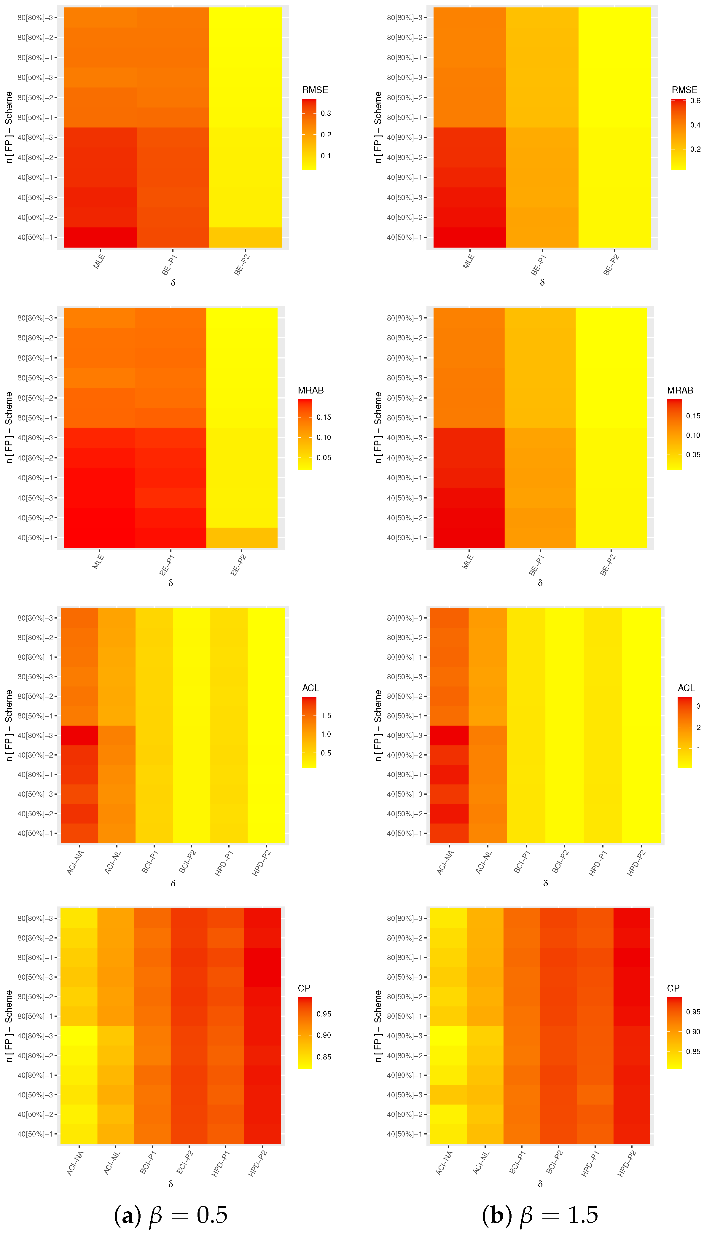
• The proposed point (or interval) estimates of $\beta$, $\delta$ and $R_1\left(t\right)$, for both given sets 1 and 2 perform well.
• As $n_k$ (or $m_k$) increases, all estimates operate effectively, produce superior outcomes and hold the consistency property. Equivalent behavior is also observed when the total of $S_{ki},i=1,2,\cdots ,m_k$ decreases.
• As $\beta$ and $\delta$ increase, the RMSEs and MRABs of all estimates of $\beta$, $\delta$ and $R_1\left(t\right)$ increase except for the Bayes estimates of $\delta$.
• As $\beta$ and $\delta$ increase, the ACLs of all estimates of $\beta$, $\delta$ and $R_1\left(t\right)$ increase, but their CPs decrease.
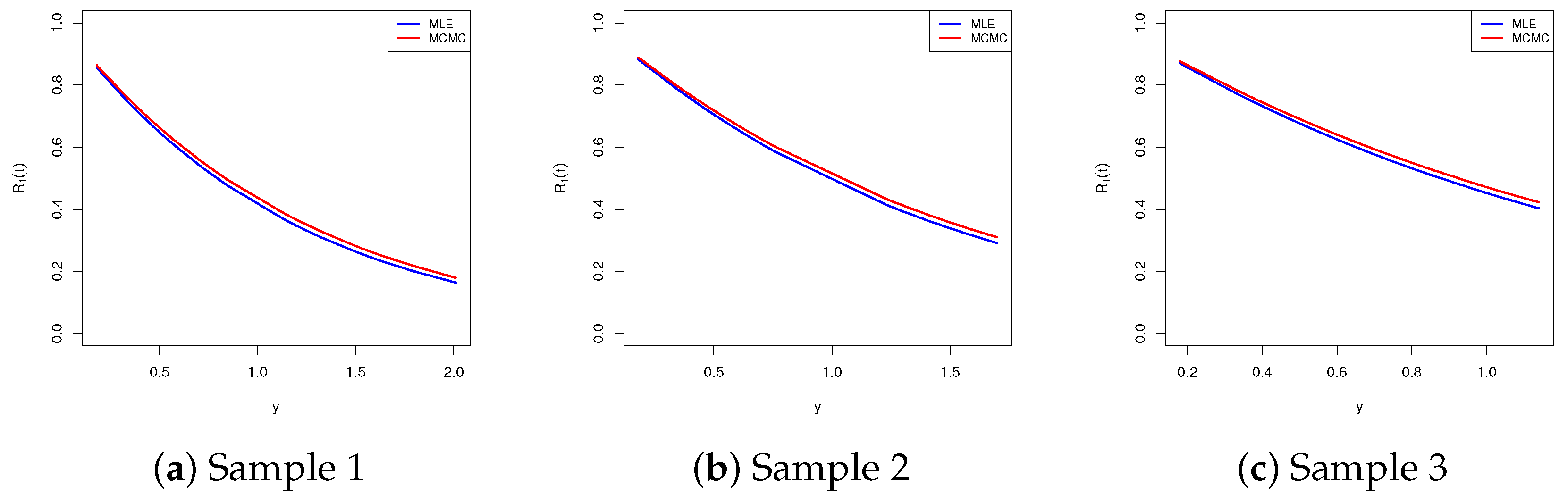
• Since the Bayes point/interval estimates included more priority information on the unknown parameters, for each setting, the Bayes estimates of $\beta$, $\delta$ or $R_1\left(t\right)$ provide more accurate results compared to those obtained from the maximum likelihood estimation method.
• Since the variance of Prior-1 is higher than that of Prior-2, as anticipated, the estimates from Prior-2 are more accurate than those based on Prior-1.
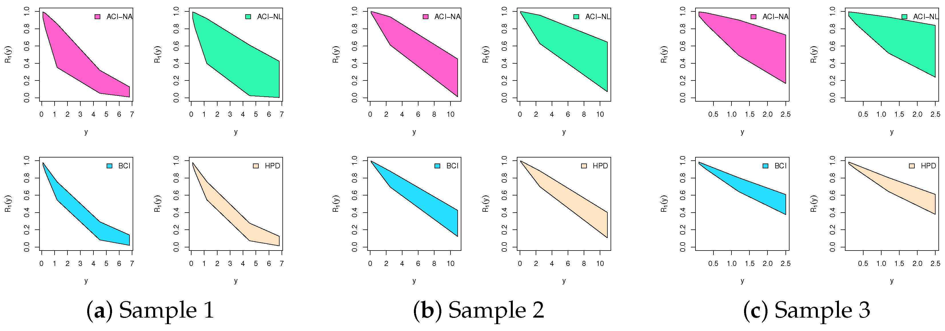
• Comparing the proposed interval estimation approaches, for both sets 1 and 2, the estimates of $\beta$ and $\delta$ derived from the ACI-NA and HPD interval methods behave preferably to the others, while the estimates of $R_1\left(t\right)$ derived from the ACI-NL and BCI methods behave better than others.
• Comparing the proposed censoring plans 1, 2 and 3, for both sets 1 and 2, it is observed that (i) the point estimates of $\beta$ and $R_1\left(t\right)$ perform better based on Scheme-2 (middle censoring) while those associated with the acceleration factor $\delta$ perform better based on Scheme-3 (right censoring) than others; and (ii) the interval estimates of $\beta$ perform better based on Scheme-3 (right censoring) while those associated with $\delta$ and $R_1\left(t\right)$ perform better based on Scheme-2 (middle censoring) than others.
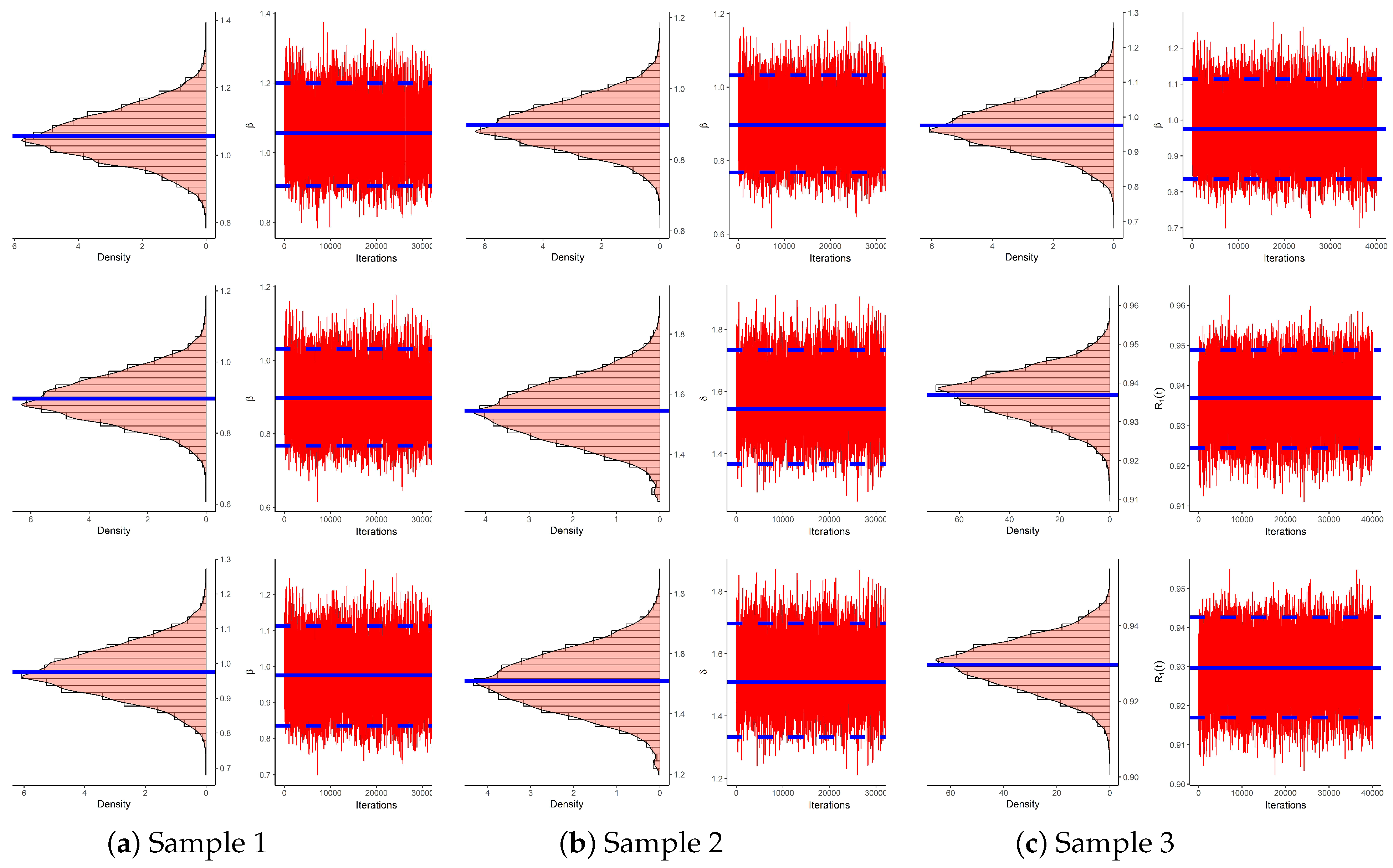
• Based on the Markov chain Monte Carlo algorithm, the Bayes estimation approach is the best choice for estimating the XL distribution parameter, its acceleration factor, and its reliability function under normal use conditions for CSPALT in the presence of PT-IIC data.

6. Applications

To show how our proposed model works in practice and for illustrative reasons, this section offers the analysis of two different accelerated data sets.

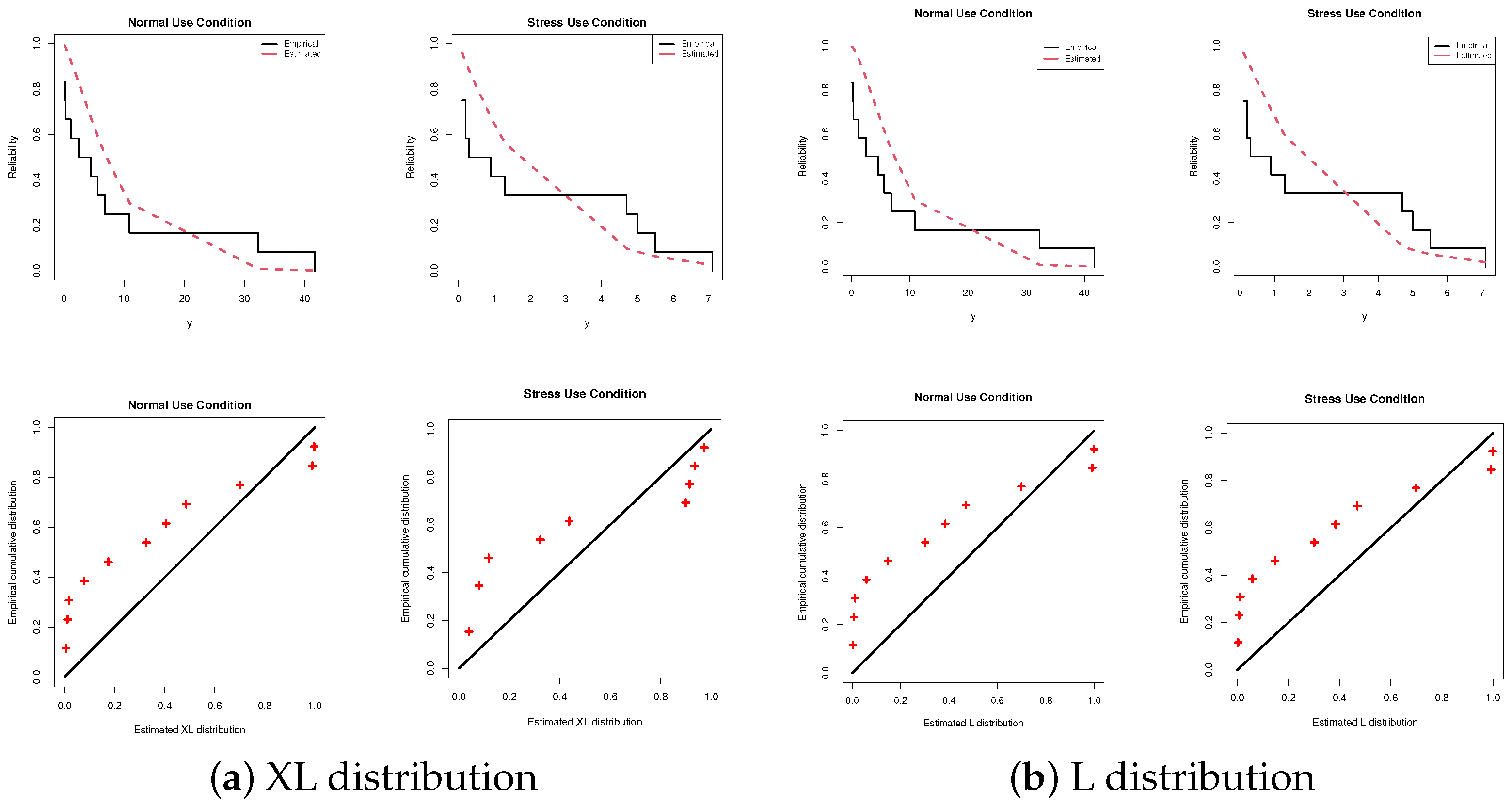
6.1. Insulating Fluid

This application offers an analysis of the time-to-breakdown (in seconds) of an insulating fluid from a voltage endurance test against different stress levels. From Nelson [26], two stress levels each containing twelve observations are considered: namely, 40 Kilovolt (normal use) and 45 Kilovolt (accelerated stress). For computational convenience, for both sets, each time point is divided by ten. In

Table 1. Times to breakdown of insulating fluid.

Normal Use (40 kV)
0.1	0.1	0.2	0.3	1.2	2.5	4.5	5.6	6.8	10.9	32.3	41.7
Accelerated Stress (45 kV)
0.1	0.1	0.1	0.2	0.2	0.3	0.9	1.3	4.7	5.0	5.5	7.1

, the newly transformed insulating fluid data sets are presented.

To check whether or not the XL distribution provides a proper fit to the insulating fluid data, the Kolmogorov–Smirnov (KS) statistic along with its p-value are considered. Briefly, using negative log-likelihood (NL), Akaike (A), consistent Akaike (CA), Bayesian (B) and Hannan–Quinn (HQ) information criteria, we compare the applicability of XL distribution with Lindley (L) distribution. From Table 1, to make this comparison, the MLE (standard error (St.E)) of XL (or L) parameter $\beta$ under normal use and accelerated stress data are calculated and reported in

Table 2. Summary fit of the XL and L distributions from insulating fluid data.

Model	Estimate(St.E)	NL	A	CA	B	HQ	KS(p-Value)
Normal Use Data
XL	0.1942(0.0401)	41.954	85.908	86.308	86.393	85.728	0.3382(0.1284)
L	0.2066(0.0425)	43.983	89.966	90.366	90.451	89.787	0.3574(0.0931)
Stress Use Data
XL	0.6507(0.1431)	21.675	45.351	45.751	45.836	45.172	0.3815(0.0607)
L	0.7408(0.1586)	22.859	47.719	48.119	48.204	47.540	0.4029(0.0406)

. It shows that the XL distribution has the smallest values of NL, A, CA, B, HQ, KS statistics and the highest p-value. As a result, the XL distribution provides a better fit than the L distribution for both given normal use and accelerated stress data sets. It is also indicates that the XL distribution fits the insulating fluid data well for both stress levels. Using the two data sets, in Figure 6, the fitted/empirical reliability functions and probability–probability (PP) plots for XL and L lifetime models are displayed. It shows that the proposed XL model offers a good fit to the insulating fluid data sets and supports the same goodness-of-fit findings.

Now, to demonstrate the feasibility of the proposed methodologies, several PT-IIC samples from the insulating fluid data sets are created. From Table 1, taking $m_1=m_2=6$, three artificial samples based on various progressive censoring patterns $S_{ki}=S_{ki},i=1,2,\cdots ,m_k,k=1,2$ are obtained and listed in

Table 3. Various PC-T-II samples from insulating fluid data.

Sample	$\{{\mathit{S}}_{1\mathit{i}};{\mathit{S}}_{2\mathit{i}}\}$	Censored Data
1	$(6,0^5)$	0.1, 0.2, 0.3, 1.2, 4.5, 6.8
	$(6,0^5)$	0.1, 0.2, 0.3, 0.9, 1.3, 5.0
2	$(0^2,3,3,0^2)$	0.1, 0.1, 0.2, 0.3, 2.5, 10.9
	$(0^2,3,3,0^2)$	0.1, 0.1, 0.1, 0.2, 0.9, 5.0
3	$(0^5,6)$	0.1, 0.1, 0.2, 0.3, 1.2, 2.5
	$(0^5,6)$	0.1, 0.1, 0.1, 0.2, 0.2, 0.3

. Here, for brevity, the scheme $(6,0,0,0,0,0)$ is referred to as $(6,0^5)$. So, for each generated sample, the classical estimates (with their ACIs through NA and NL approaches) as well as the Bayes estimates (with their interval estimates through BCI and HPD interval approaches) of $\beta ,\delta$ and $R_1\left(t\right)$ (at distinct time $t=0.5$) are calculated and displayed in

Table 4. Point estimates of $\beta$, $\delta$ and $R_1\left(t\right)$ from insulating fluid data.

Sample	Par.	MLE		MCMC
		Est.	St.E	Est.	St.E
1	$\beta$	0.6285	0.1904	0.5658	0.0991
	$\delta$	1.5970	0.9144	1.4849	0.1506
	$R_1\left(0.5\right)$	0.8169	0.0718	0.8405	0.0373
2	$\beta$	0.2316	0.0613	0.2179	0.0379
	$\delta$	2.2039	1.2641	2.1514	0.0869
	$R_1\left(0.5\right)$	0.9586	0.0181	0.9622	0.0108
3	$\beta$	0.4988	0.1420	0.4635	0.0656
	$\delta$	7.5727	4.4921	7.5226	0.0856
	$R_1\left(0.5\right)$	0.8658	0.0532	0.8788	0.0243

and

Table 5. Interval estimates of $\beta$, $\delta$ and $R_1\left(t\right)$ from insulating fluid data.

Sample	Par.	ACI-NA			BCI
		ACI-NL			HPD
		Lower	Upper	Length	Lower	Upper	Length
1	$\beta$	0.2553	1.0017	0.7463	0.4204	0.7208	0.3004
		0.3471	1.1380	0.7909	0.4152	0.7137	0.2985
	$\delta$	0.0000	3.3892	3.3892	1.2884	1.6811	0.3927
		0.5200	4.9053	4.3853	1.2961	1.6841	0.3881
	$R_1\left(0.5\right)$	0.6762	0.9576	0.2814	0.7823	0.8949	0.1126
		0.6876	0.9704	0.2828	0.7849	0.8968	0.1118
2	$\beta$	0.1116	0.3517	0.2401	0.1532	0.2906	0.1374
		0.1379	0.3890	0.2511	0.1506	0.2875	0.1369
	$\delta$	0.0000	4.6815	4.6815	2.0222	2.2885	0.2663
		0.7161	6.7830	6.0669	2.0186	2.2839	0.2653
	$R_1\left(0.5\right)$	0.9231	0.9942	0.0711	0.9402	0.9796	0.0394
		0.9237	0.9949	0.0711	0.9415	0.9805	0.0390
3	$\beta$	0.2204	0.7771	0.5567	0.3573	0.5742	0.2169
		0.2854	0.8715	0.5860	0.3561	0.5717	0.2156
	$\delta$	0.0000	16.377	16.377	7.3921	7.6590	0.2669
		2.3676	24.221	21.853	7.3874	7.6538	0.2664
	$R_1\left(0.5\right)$	0.7615	0.9702	0.2087	0.8373	0.9175	0.0801
		0.7675	0.9767	0.2092	0.8403	0.9199	0.0796

, respectively. Due to there being no available prior information about $\beta$ or $\delta$, we set $a_k$ and $b_k$ for $k=1,2$ as 0.001 which implies that the prior densities are almost improper. According to the MCMC methodology, we repeat the procedure 50,000 times and discard the first 10,000 iterations as burn-in. The starting values of $\beta$ and $\delta$ used to run the MCMC sampler are assumed to be their MLEs. As we anticipated, from Table 4, the acquired estimates $\beta$, $\delta$, or $R_1\left(t\right)$ exhibit similar performance that appears to be close to each other. Similar behavior is also observed in the case of interval estimates of the unknown parameters. Comparing the proposed estimation methods in terms of their lowest St.Es, it can be seen that the Bayes estimates perform better than the estimates derived from the likelihood method. On the other hand, comparing the proposed estimation methods in terms of shortest interval lengths, it is noted that the ACI-NA (in the classical point of view) and HPD intervals (in the Bayes point of view) behave superior when compared to others.

One of the main issues when using the MCMC procedure is how to prove the convergence of Markovian chains. For this purpose, from the remaining 40,000 MCMC variates in each generated sample, a trace plot (which furnishes an essential tool for evaluating the mixing of a chain) and density plot (which provides a smoothed histogram of outputs) are shown in Figure 7. For each plot in Figure 7, the Bayes estimate of $\beta$, $\delta$ or $R_1\left(t\right)$ is represented by a solid (–) line. Additionally, the HPD interval bounds of the unknown quantities are represented by dashed (- - -) lines. We see, from Figure 7, that (i) the simulated MCMC estimates converged well, (ii) the burn-in sample has sufficient size to eliminate the effect of the initial points, and (iii) the density distribution of $\beta$, $\delta$ or $R_1\left(t\right)$ is almost fairly symmetrical, except the density of $R_1\left(t\right)$ from Sample 2 is negatively-skewed.

From 40,000 MCMC outputs simulated from each artificial sample reported in Table 3,

Table 6. Characteristics of $\beta$, $\delta$ and $R_1\left(t\right)$ from insulating fluid data.

Sample	Par.	Mean	Mode	${\mathcal{Q}}_1$	${\mathcal{Q}}_2$	${\mathcal{Q}}_3$	St.D	Skewness
1	$\beta$	0.56582	0.50241	0.51437	0.56481	0.61539	0.07681	0.12627
	$\delta$	1.48493	1.20282	1.41684	1.48423	1.55349	0.10058	0.00933
	$R_1\left(0.5\right)$	0.84050	0.86443	0.82182	0.84093	0.85994	0.02883	–0.13522
2	$\beta$	0.21794	0.22567	0.19290	0.21625	0.24110	0.03536	0.25698
	$\delta$	2.15143	1.94905	2.10374	2.14982	2.19832	0.06928	0.06757
	$R_1\left(0.5\right)$	0.96221	0.96039	0.95581	0.96312	0.96960	0.01020	–0.49041
3	$\beta$	0.46348	0.38443	0.42646	0.46216	0.50003	0.05536	0.10422
	$\delta$	7.52261	7.37523	7.47489	7.52122	7.57016	0.06935	0.05224
	$R_1\left(0.5\right)$	0.87879	0.90788	0.86532	0.87946	0.89264	0.02049	–0.15533

presents useful characteristics of $\beta$, $\delta$ and $R_1\left(t\right)$: namely, mean, mode, quartiles (${\mathcal{Q}}_i,i=1,2,3$, standard deviation (St.D) and skewness. It is clear that the calculated properties of $\beta$, $\delta$ and $R_1\left(t\right)$ listed in Table 6 support our findings in Figure 7.

To demonstrate the performance of the reliability parameter $R_1\left(y\right)$, at the full normal use data points in Samples 1, 2 and 3, the MLEs and Bayes estimates of $R_1\left(y\right)$ are shown in Figure 8, while its interval estimates developed by ACI-NA, ACI-NL, BCI and HPD interval approaches are shown in Figure 9. Figure 8 showed that the estimates of $R_1\left(y\right)$ developed from the MCMC method are greater than those developed from the maximum likelihood method. In addition, Figure 9 indicated that the interval estimates of $R_1\left(y\right)$ developed from the ACI-NA method have smaller interval lengths than its competitor ACI-NL method, while those obtained from BCI and HPD interval methods are quite near to each other. As a result, the detailed findings created from the insulating fluid data support the same conclusions drawn in Section 5.

6.2. Light-Emitting Diode

A Light-Emitting Diode (or simply LED) is a semiconductor device that emits infrared or visible light when charged with an electric current. Visible LEDs are used in many electronic devices as indicator lamps, e.g., street lights, parking garage lighting, billboards, signs, etc.

Table 7. Failure times of 58 LED products.

Normal Use Condition
0.18, 0.19, 0.19, 0.34, 0.36, 0.40, 0.44, 0.44, 0.45, 0.46, 0.47, 0.53, 0.57, 0.57, 0.63,
0.65, 0.70, 0.71, 0.71, 0.75, 0.76, 0.76, 0.79, 0.80, 0.85, 0.98, 1.01, 1.07, 1.12, 1.14,
1.15, 1.17, 1.20, 1.23, 1.24, 1.25, 1.26, 1.32, 1.33, 1.33, 1.39, 1.42, 1.50, 1.55, 1.58,
1.59, 1.62, 1.68, 1.70, 1.79, 2.00, 2.01, 2.04, 2.54, 3.61, 3.76, 4.65, 8.97
Accelerated Stress Condition
0.13, 0.16, 0.20, 0.20, 0.21, 0.25, 0.26, 0.28, 0.28, 0.30, 0.31, 0.33, 0.35, 0.35, 0.35,
0.39, 0.50, 0.52, 0.58, 0.60, 0.60, 0.62, 0.63, 0.67, 0.71, 0.73, 0.75, 0.75, 0.78, 0.80,
0.80, 0.86, 0.90, 0.91, 0.93, 0.93, 0.94, 0.98, 0.99, 1.01, 1.03, 1.06, 1.06, 1.10, 1.22,
1.22, 1.24, 1.28, 1.39, 1.39, 1.46, 1.48, 1.52, 1.74, 1.95, 2.46, 3.02, 5.16

displays the failure time (at 1000 h) created under normal use and accelerated stress conditions, each involving 58 time points. The LED data have been discussed by Cheng and Wang [27] and recently analyzed by Dey et al. [9] and Nassar and Elshahhat [22]. To examine if the XL distribution is an adequate model to fit the LED data or not, the KS distance and its p-value at are considered. Firstly, from Table 7, the MLE (standard error) of $\beta$ from use and stress data sets are 0.9502 (0.0992) and 1.2852 (0.1393), respectively. Then, utilizing Table 7, the KS(p-Value) for both complete LED data sets from use and stress conditions are computed as 0.1659 (0.082) and 0.1541 (0.127), respectively. As a result, the XL lifetime model fits the LED data appropriately. For more clarification, Figure 10 displays the estimated/empirical RFs and PP plots from use and stress LED data sets. This means that the XL model offers an adequate fit for LED data.

Currently, to show the acquired point and interval estimators of XL parameters $\beta$ and $R_1\left(t\right)$ as well as the acceleration factor $\delta$, three different PT-IIC samples from the original LED data sets are generated and presented in

Table 8. Various PC-T-II samples from LED data.

Sample	$\{{\mathit{S}}_{1\mathit{i}};{\mathit{S}}_{2\mathit{i}}\}$	Censored Data
1	$(28,0^{29})$	0.18, 0.19, 0.19, 0.34, 0.36, 0.40, 0.44, 0.44, 0.45, 0.46, 0.47, 0.53, 0.57, 0.71, 0.71,
		0.75, 0.85, 1.14, 1.17, 1.20, 1.32, 1.33, 1.50, 1.55, 1.58, 1.59, 1.62, 1.79, 2.00, 2.01
	$(28,0^{29})$	0.13, 0.16, 0.20, 0.25, 0.26, 0.28, 0.28, 0.30, 0.35, 0.35, 0.60, 0.62, 0.63, 0.67, 0.71,
		0.73, 0.75, 0.75, 0.80, 0.80, 0.86, 0.90, 0.98, 0.99, 1.01, 1.22, 1.24, 1.28, 1.39, 1.39
2	$(0^{14},14,14,0^{14})$	0.18, 0.19, 0.19, 0.34, 0.36, 0.40, 0.44, 0.44, 0.45, 0.46, 0.47, 0.53, 0.57, 0.57, 0.63,
		0.65, 0.70, 0.71, 0.71, 0.75, 0.76, 0.76, 1.23, 1.26, 1.32, 1.42, 1.55, 1.59, 1.68, 1.70
	$(0^{14},14,14,0^{14})$	0.13, 0.16, 0.20, 0.20, 0.21, 0.25, 0.26, 0.28, 0.28, 0.30, 0.31, 0.33, 0.35, 0.35, 0.35,
		0.39, 0.50, 0.60, 0.60, 0.62, 0.71, 0.73, 0.75, 0.78, 0.90, 0.91, 0.98, 1.01, 1.03, 1.28
3	$(0^{29},28)$	0.18, 0.19, 0.19, 0.34, 0.36, 0.40, 0.44, 0.44, 0.45, 0.46, 0.47, 0.53, 0.57, 0.57, 0.63,
		0.65, 0.70, 0.71, 0.71, 0.75, 0.76, 0.76, 0.79, 0.80, 0.85, 0.98, 1.01, 1.07, 1.12, 1.14
	$(0^{29},28)$	0.13, 0.16, 0.20, 0.20, 0.21, 0.25, 0.26, 0.28, 0.28, 0.30, 0.31, 0.33, 0.35, 0.35, 0.35,
		0.39, 0.50, 0.52, 0.58, 0.60, 0.60, 0.62, 0.63, 0.67, 0.71, 0.73, 0.75, 0.75, 0.78, 0.80

, with $m_1=m_2=30$ and different choices of $S_k=S_{ki},i=1,2,\cdots ,m_k,k=1,2$.

Utilizing the data in Table 8, the MLEs and associated ACIs of $\beta$, $\delta$ and $R_1\left(t\right)$ (for $t=0.1$) are calculated. Setting $a_k,b_k=0.001,k=1,2$ in Bayes’ calculations, under the assumption that the first 10,000 of 50,000 variates from each Markov chain are discarded, the Bayes point estimates as well as the BCI/HPD interval estimates of $\beta$, $\delta$ and $R_1\left(t\right)$ (for $t=0.1$) are obtained. However, in

Table 9. Point estimates of $\beta$, $\delta$ and $R_1\left(t\right)$ from LED data.

Sample	Par.	MLE		MCMC
		Est.	St.E	Est.	St.E
1	$\beta$	1.1011	0.1637	1.0566	0.0867
	$\delta$	1.4019	0.3687	1.2951	0.1462
	$R_1\left(0.1\right)$	0.9181	0.0152	0.9222	0.0080
2	$\beta$	0.9338	0.1334	0.8975	0.0765
	$\delta$	1.6411	0.4316	1.5452	0.1354
	$R_1\left(0.1\right)$	0.9336	0.0123	0.9369	0.0071
3	$\beta$	1.0167	0.1468	0.9757	0.0815
	$\delta$	1.6052	0.4213	1.5092	0.1351
	$R_1\left(0.1\right)$	0.9259	0.0136	0.9297	0.0075

and

Table 10. Interval estimates of $\beta$, $\delta$ and $R_1\left(t\right)$ from LED data.

Sample	Par.	ACI-NA			BCI
		ACI-NL			HPD
		Lower	Upper	Length	Lower	Upper	Length
1	$\beta$	0.7802	1.4220	0.6418	0.9118	1.2071	0.2953
		0.8228	1.4737	0.6509	0.9055	1.1993	0.2939
	$\delta$	0.6792	2.1246	1.4454	1.0933	1.4869	0.3936
		0.8372	2.3475	1.5102	1.1046	1.4916	0.3870
	$R_1\left(0.1\right)$	0.8883	0.9478	0.0595	0.9083	0.9356	0.0274
		0.8888	0.9483	0.0596	0.9090	0.9362	0.0272
2	$\beta$	0.6723	1.1953	0.5230	0.7681	1.0323	0.2642
		0.7057	1.2356	0.5299	0.7680	1.0319	0.2638
	$\delta$	0.7952	2.4870	1.6918	1.3678	1.7345	0.3667
		0.9801	2.7479	1.7677	1.3678	1.7334	0.3656
	$R_1\left(0.1\right)$	0.9094	0.9578	0.0484	0.9245	0.9488	0.0244
		0.9097	0.9581	0.0484	0.9245	0.9488	0.0243
3	$\beta$	0.7290	1.3044	0.5754	0.8378	1.1165	0.2787
		0.7661	1.3493	0.5831	0.8357	1.1134	0.2776
	$\delta$	0.7795	2.4310	1.6520	1.3311	1.6965	0.3653
		0.9597	2.6850	1.7250	1.3319	1.6970	0.3651
	$R_1\left(0.1\right)$	0.8992	0.9526	0.0534	0.9166	0.9424	0.0258
		0.8996	0.9530	0.0534	0.9169	0.9426	0.0257

, the point estimates (with their St.Es) and interval estimates (with their lengths) are reported, respectively. However, the estimation results in Table 9 and Table 10 stated that the estimates of $\beta$, $\delta$ or $R_1\left(t\right)$ obtained via the maximum likelihood (or Bayes MCMC) approach are quite close to each other. However, when comparing the acquired point estimates of $\beta$, $\delta$ and $R_1\left(t\right)$, it can be seen that the Bayes estimates behave satisfactorily than the classical estimates in terms of the lowest St.Es. Equivalent behavior is also observed in the case of interval estimates.

Two MCMC plots, namely trace and density plots, are also considered in Figure 11 to evaluate the convergence of simulated Markovian chains of $\beta$, $\delta$ and $R_1\left(t\right)$ from the LED data. It shows that the estimates developed from the proposed MCMC procedure are converged adequately, and the associated densities of $\beta$, $\delta$ or $R_1\left(t\right)$ are almost symmetrical. Moreover, using 40,000 MCMC variates obtained from each unknown parameter, the same characteristics reported in Table 6 are also reused under LED data; see

Table 11. Characteristics of $\beta$, $\delta$ and $R_1\left(t\right)$ from LED data.

Sample	Par.	Mean	Mode	${\mathcal{Q}}_1$	${\mathcal{Q}}_2$	${\mathcal{Q}}_3$	St.D	Skewness
1	$\beta$	1.05659	0.97503	1.00675	1.05321	1.10589	0.07440	0.10953
	$\delta$	1.29506	1.00769	1.22867	1.29564	1.36308	0.09972	–0.07161
	$R_1\left(0.1\right)$	0.92221	0.92977	0.91763	0.92252	0.92683	0.00690	–0.10999
2	$\beta$	0.89753	1.00956	0.85154	0.89513	0.94278	0.06733	0.11433
	$\delta$	1.54519	1.26645	1.47943	1.54308	1.61046	0.09559	0.06226
	$R_1\left(0.1\right)$	0.93693	0.92657	0.93276	0.93717	0.94118	0.00621	–0.12847
3	$\beta$	0.97569	1.09249	0.92824	0.97360	1.02265	0.07043	0.10148
	$\delta$	1.50918	1.23056	1.44375	1.50729	1.57402	0.09507	0.05070
	$R_1\left(0.1\right)$	0.92970	0.91888	0.92536	0.92991	0.93411	0.00652	–0.10833

. It further supports the same findings shown in Figure 11.

To assess the actual behavior of the reliability function under normal use conditions in LED data, utilizing Samples 1, 2 and 3 reported in Table 8, both point and interval estimates of $R_1\left(y\right)$ are displayed in Figure 12 and Figure 13, respectively. It is clear, from Figure 12, that the Bayes estimates have higher-level values than the classical estimates. In addition, Figure 13 showed that the asymptotic interval estimates (developed by NA/NL) are quite close to each other. A similar pattern is also noted in the case of the Bayes interval estimates (developed by BCI/HPD interval). Furthermore, in terms of the smallest interval length, the HPD (or BCI) interval estimates perform better compared to the ACI-NA (or ACI-NL) estimates. Obviously, the interval estimates of $R_1\left(y\right)$ in Figure 8 are smoother than those in Figure 13 because the LED data have a larger size than those created from the insulating fluid data.

In conclusion, the findings obtained from insulating fluid or LED data revealed that the proposed XL lifetime model is beneficial for addressing engineering issues and demonstrated the applicability of the suggested estimation techniques to real phenomena.

7. Concluding Remarks

An investigation of constant-stress partially accelerated life tests when the lifetime of the test product follows the XLindley distribution is presented in this paper. Utilizing the progressive Type-II censored sample, two approaches are considered to obtain the point and interval estimators for the unknown parameters and the reliability function at the normal use conditions. In addition to the maximum likelihood estimates, two approximate confidence intervals are obtained based on the asymptotic normality of the maximum likelihood estimates. From the Bayesian point of view, the point estimates of the different parameters are acquired using the Monte Carlo Markov Chain technique based on the squared error loss function. The Bayes credible intervals and highest posterior density credible intervals are also provided. A simulation study and two applications are provided to compare the various estimators and demonstrate the effectiveness of the suggested approaches. The numerical outcomes showed that the estimates produced by the Bayesian approach are more accurate than those produced by the maximum likelihood estimation method in terms of minimum root mean squared error, relative absolute biase and interval length. For the model parameter and the acceleration factor, the highest posterior density credible interval procedure gives the smallest interval lengths compared to other methods. Alternatively, to obtain the reliability interval bounds under normal use conditions, the Bayes credible interval is preferred. In future work, it is of interest to investigate the estimation issues of the same model used in the current study in the presence of other censoring schemes, such as adaptive progressive censoring or generalized progressive hybrid censoring. Another future work is to compare the efficiency of Bayesian estimations based on symmetric and asymmetric loss functions, including LINEX and general entropy loss functions.

References

1. El-Din, M.M.; Abu-Youssef, S.E.; Ali, N.S.; El-Raheem, A.A. Estimation in constant-stress accelerated life tests for extension of the exponential distribution under progressive censoring. Metron 2016, 74, 253–273. [Google Scholar] [CrossRef]
2. Samanta, D.; Ganguly, A.; Kundu, D.; Mitra, S. Order restricted Bayesian inference for exponential simple step-stress model. Commun.-Stat.-Simul. Comput. 2017, 46, 1113–1135. [Google Scholar] [CrossRef]
3. Wang, L. Inference of constant-stress accelerated life test for a truncated distribution under progressive censoring. Appl. Math. Model. 2017, 44, 743–757. [Google Scholar] [CrossRef]
4. Cui, W.; Yan, Z.; Peng, X. Statistical analysis for constant-stress accelerated life test with Weibull distribution under adaptive Type-II hybrid censored data. IEEE Access 2019, 7, 165336–165344. [Google Scholar] [CrossRef]
5. Nassar, M.; Okasha, H.; Albassam, M. E-Bayesian estimation and associated properties of simple step–stress model for exponential distribution based on type-II censoring. Qual. Reliab. Eng. Int. 2021, 37, 997–1016. [Google Scholar] [CrossRef]
6. Kumar, D.; Nassar, M.; Dey, S.; Alam, F.M.A. On estimation procedures of constant stress accelerated life test for generalized inverse Lindley distribution. Qual. Reliab. Eng. Int. 2022, 38, 211–228. [Google Scholar] [CrossRef]
7. Hyun, S.; Lee, J. Constant-stress partially accelerated life testing for log-logistic distribution with censored data. J. Stat. Appl. Probab. 2015, 4, 193–201. [Google Scholar]
8. Mohamed, N.M. Estimation on kumaraswamy-inverse Weibull distribution with constant stress partially accelerated life tests. Appl. Math. Inf. Sci. 2021, 15, 503–510. [Google Scholar]
9. Dey, S.; Wang, L.; Nassar, M. Inference on Nadarajah–Haghighi distribution with constant stress partially accelerated life tests under progressive type-II censoring. J. Appl. Stat. 2022, 49, 2891–2912. [Google Scholar] [CrossRef]
10. Eliwa, M.S.; Ahmed, E.A. Reliability analysis of constant partially accelerated life tests under progressive first failure type-II censored data from Lomax model: EM and MCMC algorithms. AIMS Math. 2023, 1, 29–60. [Google Scholar] [CrossRef]
11. Almarashi, A.M. Inferences of generalized inverted exponential distribution based on partially constant-stress accelerated life testing under progressive Type-II censoring. Alex. Eng. J. 2023, 63, 223–232. [Google Scholar] [CrossRef]
12. Rastogi, M.K.; Tripathi, Y.M. Estimating the parameters of a Burr distribution under progressive type II censoring. Stat. Methodol. 2012, 9, 381–391. [Google Scholar] [CrossRef]
13. Sultan, K.S.; Alsadat, N.H.; Kundu, D. Bayesian and maximum likelihood estimations of the inverse Weibull parameters under progressive type-II censoring. J. Stat. Comput. Simul. 2014, 84, 2248–2265. [Google Scholar] [CrossRef]
14. Wu, M.; Gui, W. Estimation and prediction for Nadarajah-Haghighi distribution under progressive type-II censoring. Symmetry 2021, 13, 999. [Google Scholar] [CrossRef]
15. Alotaibi, R.; Nassar, M.; Rezk, H.; Elshahhat, A. Inferences and engineering applications of alpha power Weibull distribution using progressive type-II censoring. Mathematics 2022, 10, 2901. [Google Scholar] [CrossRef]
16. Bedbur, S.; Mies, F. Confidence bands for exponential distribution functions under progressive type-II censoring. J. Stat. Comput. Simul. 2022, 92, 60–80. [Google Scholar] [CrossRef]
17. Balakrishnan, N. Progressive censoring methodology: An appraisal. Test 2007, 16, 211–259. [Google Scholar] [CrossRef]
18. Lindley, D.V. Fiducial distributions and Bayes’ theorem. J. R. Stat. Soc. Ser. B 1958, 20, 102–107. [Google Scholar] [CrossRef]
19. Chouia, S.; Zeghdoudi, H. The XLindley Distribution: Properties and Application. J. Stat. Theory Appl. 2021, 20, 318–327. [Google Scholar] [CrossRef]
20. Pareek, B.; Kundu, D.; Kumar, S. On Progressively censored competing risks data for Weibull distributions. Comput. Stat. Data Anal. 2009, 53, 4083–4094. [Google Scholar] [CrossRef]
21. Maiti, K.; Kayal, S.; Kundu, D. Statistical Inference on the Shannon and Rényi Entropy Measures of Generalized Exponential Distribution Under the Progressive Censoring. SN Comput. Sci. 2022, 3, 1–21. [Google Scholar] [CrossRef]
22. Nassar, M.; Elshahhat, A. Statistical Analysis of Inverse Weibull Constant-Stress Partially Accelerated Life Tests with Adaptive Progressively Type I Censored Data. Mathematics 2023, 11, 370. [Google Scholar] [CrossRef]
23. Henningsen, A.; Toomet, O. maxLik: A package for maximum likelihood estimation in R. Comput. Stat. 2011, 26, 443–458. [Google Scholar] [CrossRef]
24. Plummer, M.; Best, N.; Cowles, K.; Vines, K. CODA: Convergence diagnosis and output analysis for MCMC. R News 2006, 6, 7–11. [Google Scholar]
25. Balakrishnan, N.; Cramer, E. The Art of Progressive Censoring; Spriger: New York, NY, USA; Birkhäuser: Basel, Switzerland, 2014. [Google Scholar]
26. Nelson, W.B. Accelerated Testing: Statistical Model, Test Plan and Data Analysis; Wiley: New York, NY, USA, 2004. [Google Scholar]
27. Cheng, Y.F.; Wang, F.K. Estimating the Burr XII parameters in constant–stress partially accelerated life tests under multiple censored data. Commun. Stat. -Simul. Comput. 2012, 41, 1711–1727. [Google Scholar] [CrossRef]
Figure 1. The log-likelihood function and the associated first derivative of β .
Mathematics 11 01331 g001
Figure 2. The full conditional distribution of β .
Mathematics 11 01331 g002
Figure 3. Heat-map for the Monte Carlo results of β .
Mathematics 11 01331 g003
Figure 4. Heat-map for the Monte Carlo results of δ .
Mathematics 11 01331 g004
Figure 5. Heat-map for the Monte Carlo results of R 1 ( t ) .
Mathematics 11 01331 g005
Figure 6. Fitted reliability (top) and PP (bottom) plots from insulating fluid data.
Mathematics 11 01331 g006
Figure 7. Density (left) and Trace (right) plot of β , δ and R 1 ( t ) from insulating fluid data.
Mathematics 11 01331 g007
Figure 8. Point estimates of R 1 ( y ) from insulating fluid data.
Mathematics 11 01331 g008
Figure 9. Interval estimates of R 1 ( y ) from insulating fluid data.
Mathematics 11 01331 g009
Figure 10. Fitted reliability (left) and PP (right) plots from LED data.
Mathematics 11 01331 g010
Figure 11. Density (left) and Trace (right) plot of β , δ and R 1 ( t ) from LED data.
Mathematics 11 01331 g011
Figure 12. Point estimates of R 1 ( y ) from LED data.
Mathematics 11 01331 g012
Figure 13. Interval estimates of R 1 ( y ) from LED data.
Mathematics 11 01331 g013