Spread Prediction and Classification of Asian Giant Hornets Based on GM-Logistic and CSRF Models

Abstract

As an invasive alien species, Asian giant hornets are spreading rapidly and widely in Washington State and have caused significant disturbance to the daily life of residents. Therefore, this paper studies the hornets’ spread and classification models based on the GM-Logistic and CSRF models, which are significant for using limited resources to control pests and protect the ecological environment. Firstly, by combining the improved grey prediction model (GM) with the logistic model, this paper proposes a GM-Logistic model to obtain hornets’ spread rules regarding spatial location distribution and population quantity. The GM-Logistic model has higher accuracy and better fitting effect when only a few non-equally spaced sequences data are used for prediction. Secondly, a cost-sensitive random forest (CSRF) model was proposed to solve the problems of hornets’ classification and priority survey decisions in unbalanced datasets. The hornets’ binary classification model was established through feature extraction, the transformation from an unbalanced dataset to a balanced dataset, and the training dataset. CSRF improves the adaptability and robustness of the original classifier and provides a better classification effect on unbalanced datasets. CSRF outperforms the Random Forest, Classification and Regression Trees, and Support Vector Machines in performance evaluation indexes such as classification accuracy, G-mean, F1-measure, ROC curve, and AUC value. Thirdly, this paper adds human control factors and cycle parameters to the logistic model, obtaining the judgment conditions of report update frequency and pest elimination. Finally, the goodness-of-fit test on each model shows that the models established in this paper are feasible and reasonable.

1. Introduction

In March 2020, colonization of Asian giant hornets was discovered in Washington State [1,2]. Although the nest was quickly destroyed, news of the incident quickly spread throughout the area, causing much panic among residents. The spread of Asian giant hornets in Washington State exhibits a rapid and widespread trend. However, the spread prediction and classification of these pests is not satisfactory, and this will affect the scientific decision making of the government and the implementation of related policies [3].

The Asian giant hornets found in Washington state belong to a species of wasp from China that is four times larger than the bees native to Britain and France, making it the largest wasp species in the world [4]. It is characterized by a striking color, with a yellow head, a black–brown-striped belly, and a black thorax [5]. These hornets are predators of European bees that invade and destroy their nests. A small number of hornets can wipe out entire European colonies in a short time, resulting in a severe drop in honey production. As a result, they are considered locally to be an invasive alien species [6]. Moreover, this kind of hornet is aggressive and can cause stings that may lead to the death of people as a result of allergies [7]. The sudden appearance of Asian giant hornets has caused great damage to the local bee ecology and threatened residents’ lives.

Since Asian giant hornets belong to a natural population, scholars assume their biological characteristics to be like those of other common insects and bees [8]. The existing research on the spread and prediction models of Asian giant hornets has mainly adopted quantitative methods based on ecology or differential equations such as spatio-temporal dynamic models of insect populations, matrix prediction models, logistic models, grey prediction analysis, neural network models, cellular automata models, species distribution models, and so on [9,10,11,12,13]. These models are based on simplified statistical models or single application scenarios to infer the spatio-temporal distribution trend of insect populations, resulting in a weak generalization of models and low prediction accuracy [14,15].

In practice, the data used for the prediction model may be incomplete, and the time interval may not be continuous. However, there is little research on prediction models in this area [16,17]. Grey system analysis is a new method for studying problems with little data and poor information, which can make credible predictions based on a small amount of historical information [2,18]. Liu and Liu [19] developed a pine bee life table to understand the changing patterns affecting their populations. They used the analytical theory of developmental dynamics in grey systems to make predictions. This method overcomes the shortcomings arising from the large amount of data and computation inherent in traditional modeling. This provides a new method for predicting the dispersion of future insect populations. In actual insect population spread and prediction models, a large amount of data of non-equally spaced sequences must be fitted and predicted. Zhang [18] proposed a non-equally spaced GM(1,1) model with asymptotic optimization of grey derivatives using a weighted average of forwarding and backward difference quotients instead of grey derivatives. The new model was demonstrated, for example, to have higher accuracy in predicting insect population dispersal [20,21]. Therefore, based on previous work, by combining the improved grey prediction model (GM) with the logistic model, this paper proposes a GM-Logistic model to obtain the spread rules of hornets regarding spatial location distribution and population quantity. The GM-Logistic model retains the advantages of the grey prediction algorithm in solving the problems of few data and high uncertainty.

The logistic equation is a classical ecological model that points out the basic law of population growth in finite space and is able to achieve remarkable results in predicting the spatio-temporal dynamic relationship of insect populations. Still, the traditional logistic model is not ideal for prediction in complex situations [22,23,24,25]. The improvement of the logistic model in recent years has mainly centered around correcting equations, fitting parameters, and optimal harvesting strategy [26,27]. The life cycle of the Asian giant hornet is similar to that of several other hornets. Every spring, the queen bee appears after fertilization and starts a new bee colony. In autumn, the new queen bee leaves her nest to spend the winter in the soil and waits for the arrival of spring. The new queen bee builds her nest in the range of 30 km [28,29]. Therefore, this paper adds human control factors and cycle parameters based on diffusion law to the logistic model, obtaining report update frequency and the judgment condition for pest elimination. Our experiments show that the GM-Logistic model is more consistent with invasive alien species’ ecological reproduction law and has a good prediction effect. We find that the population size of hornets fluctuates around the threshold over time, and there is a periodic phenomenon.

The Washington state government has set up a hotline and website for people to report any potential clues about the wasps [30,31,32]. According to the Asian Hornet Public Dashboard (Washington State Department of Agriculture 2020), from September 2019 to December 2020, the Washington state government collected 4440 eyewitness reports of suspected Asian hornets and investigated 2098 of those sightings. Although the government investigated 2098 eyewitness report, only 14 were ultimately confirmed as being Asian giant hornets. In other words, most of the insects in the eyewitness reports were not Asian hornets but other species of insects [33]. The dataset of eyewitness reports received from the residents is a typical unbalanced dataset, where the number of samples in the positive category is much smaller than the number of samples in the negative category (which can be downloaded from the web page: https://www.comap-math.com/mcm/2021MCM_ProblemC_Files.rar (accessed on 1 December 2022); a password is required to open the file: Af6SP7rdm33PxPJmDb4wZq7cw). Since traditional machine learning methods such as SVM and Decision Trees are sensitive to unbalanced data, they often fail to achieve ideal results when dealing with the classification of unbalanced datasets [6,34,35]. At the same time, the government has limited resources to manage invasive alien species like the Asian giant hornets, so the government must accurately classify and identify the Asian giant hornets from the eyewitness reports that have not yet been investigated [1,36,37].

It is significant to study the classification of Asian giant hornets in unbalanced datasets and provide a theoretical basis for the government. Random Forest is an integrated model, it has better classification accuracy for unbalanced datasets. In addition, random forest algorithms are fast and perform well when dealing with extensive data. The random forest algorithm does not need to worry about the problem of multicollinearity faced by general regression analysis and does not have to make variable selection [38,39,40]. Although there are many studies on insect classification, few studies on using the cost-sensitive random forest solve insect classification in unbalanced datasets from the perspective of algorithms. Therefore, this paper proposes a CSRF model to solve hornets’ classification and priority survey decisions in unbalanced datasets. A binary classification model for the hornets is established through feature extraction, the transformation of an unbalanced dataset into a balanced dataset, and the training dataset. The model is able to solve the problem of poor classification effects of unbalanced datasets. Moreover, it improves the adaptability and robustness of the original classifier and has a good classification effect for unbalanced datasets.

Compared with previous research methods on the spread and classification of Asian hornets, this paper makes the following four contributions:

(I)

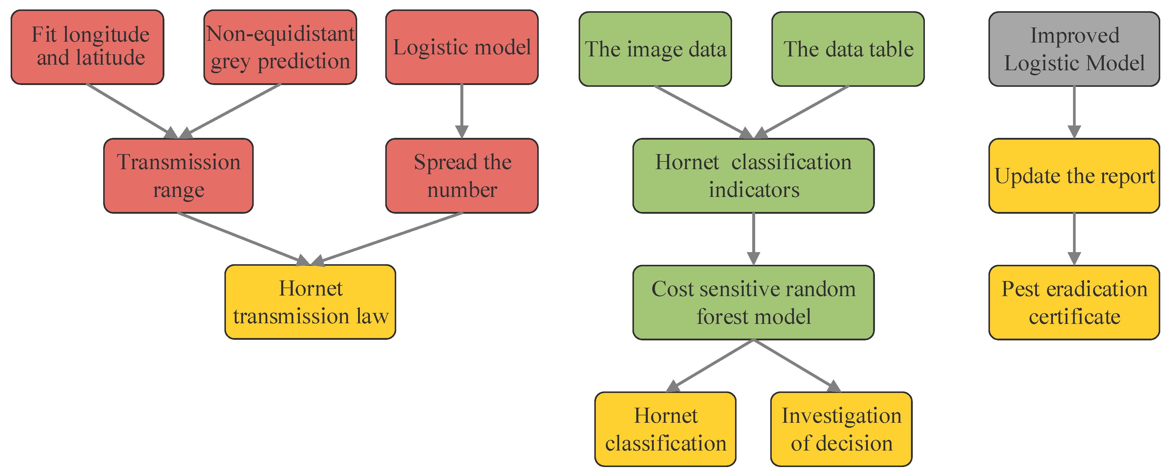
First, this paper proposes a GM-Logistic model to obtain hornets’ spread rules in terms of spatial location distribution and population quantity. An improved grey prediction model is established to predict hornets’ changes in latitude and longitude over time, and a logistic model is used to obtain the changes in the number of hornets populations over time. The GM-Logistic model retains the advantages of the grey prediction algorithm in solving the problems of little data and high uncertainty. The GM-Logistic model has higher accuracy and better fitting effect when only a few non-equally spaced time sequences data are used for prediction.

(II)

Second, a CSRF model was proposed to solve the problems of hornets’ classification and priority survey decisions in unbalanced datasets. CSRF introduces weighted Mahalanobis distance to construct cost factors in the actual class distribution, uses the same pre-test sample to determine the weight of the base classifier, and changes the majority voting system to the weighted voting system. A binary classification model was established for the hornets through feature extraction, the transformation from an unbalanced dataset to a balanced dataset, and the training dataset. The model improves the adaptability and robustness of the original classifier and provides a better classification effect on unbalanced datasets. CSRF outperforms the Random Forest, Classification and Regression Trees, and Support Vector Machines in standard performance evaluation indexes such as classification accuracy, G-mean, F1-measure, ROC curve, and AUC value.

(III)

Third, this paper adds human control factors and cycle parameters to the logistic model, which is more in line with invasive alien species’ ecological reproduction law and has a better prediction effect. We obtain the judgment conditions of report update frequency and pest elimination. The population size of wasps was found to fluctuate around a threshold value over time and there was a cyclical phenomenon.

(IV)

Fourth, the goodness-of-fit test on each model shows that the models established in this paper are feasible and reasonable. This paper provides a new theoretical basis and decision support for government departments to deal with invasive alien species.

The scheme flow chart of the proposed method in our paper is shown in Figure 1.

2. Methods

2.1. GM-Logistic Model

Based on previous work [41,42,43,44], by combining the improved grey prediction model (GM) with the logistic model, this paper proposes a GM-Logistic model to obtain hornets’ spread rules regarding spatial location distribution and population quantity. On the one hand, an improved grey prediction model is established to systematically predict hornets’ changes in latitude and longitude with time. On the other hand, a logistic model is used to obtain the changes in the number of hornets population over time.

2.1.1. Prediction of the Spread Range Based on Improved Grey Prediction Model

Due to the small amount of data (only the 14 correct data reports) in this topic, and in order to make the prediction effect more ideal, we establish an improved grey prediction model in this section. Through equal spacing processing and smoothness test, the improved grey prediction model GM(1,1) was proposed to predict the changes in longitude and latitude of hornets’ activity over time [20,21].

Step 1: Processing of non-equidistant data

The time of data is not equidistant, but the grey prediction model can only be used in the case of equidistant, so the original data need to be processed equidistantly.

Assume that the original data sequence is

$$x^{(0)}(k_i)=\{x^{(0)}(k_1),x^{(0)}(k_2),\dots ,x^{(0)}(k_n)\}$$

(1)

where n = 14 (the same below), $k_i$ is reporting date, and $x^{(0)}(k_i)$ represents the longitude and latitude sequence of 14 Asian giant hornets.

The time interval between each reporting date and the first reporting date (the time the first Asian giant hornet was found and reported) is set as

$$K_i=k_i-k_1,i=1,2,\dots ,n$$

(2)

Then the average time interval is

$$\Delta k_0=\frac{k_n-k_1}{n-1}$$

(3)

The coefficient of the unit time difference between $k_i$ and $\Delta k_0$ is

$$u(k_i)=\frac{k_i-(i-1)\Delta k_0}{\Delta k_0}$$

(4)

Find the total difference in each period:

$$\Delta x^{(0)}(k_i)=u(k_i)\{x^{(0)}(k_i)-x^{(0)}(k_{i-1})\}$$

(5)

Calculate the grey value of equidistant points:

$$Z^{(0)}(k_i)=x^{(0)}(k_i)-\Delta x^{(0)}(k_i)$$

(6)

Construct the equally spaced sequences:

$$Z^{(0)}(k_i)=\{Z^{(0)}(k_1),Z^{(0)}(k_2),\dots ,Z^{(0)}(k_n)\}$$

(7)

Make a summation of $Z^{(0)}(k_i)$ to generate (1-Ago) to generate the sequence:

$$Z^{(1)}(k_i)=\{Z^{(1)}(k_1),Z^{(1)}(k_2),\dots ,Z^{(1)}(k_n)\}$$

(8)

where $Z^{(1)}(k_i)={\displaystyle \sum _{m=1}^{k_i}{Z}^{(0)}(m)},k_i=1,2,\dots ,n$.

Step 2: Smoothness test

To ensure the feasibility of the grey model, the smoothness test of $X^{(0)}$ is required before the application of the model. The formula is as follows:

$$\rho (k_i)=\frac{Z^{(0)}(k_i)}{Z^{(0)}(k_i-1)},k_i=2,3,\dots ,n$$

(9)

where $\rho (k_i)$ is the smoothness coefficient, which can be used to test the smoothness of the sequence. If $\rho (k_i)<0.5$ is satisfied, then the GM(1,1) model can be established as being predictive. Otherwise, the data need to be translated, and the formula is as follows:

$$y^{(0)}(k_i)=Z^{(0)}(k_i)+c$$

(10)

where $y^{(0)}(k_i)$ is the data sequence after translation, $c$ is the translation level, and the appropriate one is selected so that the sequence can pass the test.

After the test, $\rho (k_i)=0.23<0.5$; the test was passed.

Step 3: Establishment of the GM(1,1) model

The original form of the GM(1,1) model is as follows:

$$Z^{(0)}(k_i)+a{Z}^{(1)}(k_i)=b$$

(11)

We set

$$E^{(1)}(k_i)=\frac{1}{2}(Z^{(1)}(k_i)+Z^{(1)}(k_i-1)$$

(12)

where $a$ is the development coefficient that represents the development trend of the estimated value of the sequence, $b$ is the grey action, which reflects the relationship between data changes, $E^{(1)}(k_i)=(E^{(1)}(2),E^{(1)}(3),\dots ,E^{(1)}(14))$ is the generated sequence by adjacent mean values of $X^{(1)}(k_i)$. Therefore, the GM(1,1) model is transformed into the following basic form:

$$Z^{(0)}(k_i)+a{E}^{(1)}(k_i)=b$$

(13)

We set

$$\hat{\alpha }={(a,b)}^T$$

(14)

$$Y={(Z^{(0)}(2),Z^{(0)}(3),\dots ,Z^{(0)}(n))}^T$$

(15)

$$B=\left[\begin{array}{cc}-E^{(1)}(2)& 1\\ -E^{(1)}(3)& 1\\ \dots & \dots \\ -Z^{(1)}(n)& 1\end{array}\right]$$

(16)

then, $\hat{\alpha }={(B^{T}B)}^{-1}{B}^{T}Y$ is the estimated parameter sequence of the grey differential Equation (12) by the least squares method, and the time response sequence of $Z^{(0)}(k_i)+a{E}^{(1)}(k_i)=b$ can be obtained as follows:

$$\widehat{Z^{(1)}}(k_i+1)=(Z^{(1)}(0)-\frac{b}{a})e^{-a{k}_i}+\frac{b}{a},k_i=1,2,\dots ,n$$

(17)

We set $Z^{(1)}(0)=Z^{(0)}(1)$, then we can get the reduced value:

$$\begin{array}{l}\stackrel{\wedge }{Z^{(0)}}(k_i+1)=\stackrel{\wedge }{Z^{(1)}}(k_i+1)-\stackrel{\wedge }{Z^{(1)}}(k_i)\\ =(1-e^a)(Z^{(0)}(1)-\frac{b}{a})e^{-a{k}_i},k_i=1,2,\dots ,n\end{array}$$

(18)

2.1.2. Prediction of the Spread Quantity Based on the Logistic Model

Since Asian giant hornets belong to a natural population, we assume that their biological evolution is similar to that of other common insects and bees. Therefore, for the spread quantity of Asian giant hornets, we establish a logistic population growth model to predict it.

According to relevant literature [45], hornets in a honeycomb will die around December in winter, leaving only the queen to hibernate. In spring, the queen will come out to build the nest and lay eggs, and only the fertilized queen bees can lay eggs. By August, the number of worker bees is at its peak, at about 100, and September is the month when males and queens are born, so we assume that the breeding of Asian giant hornets starts in early March. Because the number of males and queens is already low, the queen bee is likely to fight off the males, with a 65% chance of failure to fertilize.

Therefore, we take a cycle of a year and assume that the initial number of hornets in a hive is $N(0)=1$, and the maximum number of hornets is $N_{\max }=100$ by the end of August. Assume that the natural growth rate of hornets is a constant r, then $r=\frac{\Delta N(t)}{t}=\frac{100}{6}$. Thus, the logistic growth model is obtained as follows:

$$\left\{\begin{array}{l}\frac{dN}{dt}=rN(1-\frac{N}{N_{\max }})\\ N(0)=1\end{array}\right.$$

(19)

where $N(t)$ represents the number of hornets over time, r represents the growth rate of hornets, $N_{\max }$ represents the environmental capacity of hornets. Then, rN represents the growing trend of hornets, and factor $(1-N/N_{\max })$ represents the blocking effect of environment and resources.

The separation of variables method is used to solve the ordinary differential Equation (20), and the general solution is obtained as follows:

$$N(t)=\frac{N_{\max }}{1+(N_{\max }-1)e^{-rt}}$$

(20)

The life cycle of the Asian giant hornet is one year. In early March, the queen bees come out to build nests and lay eggs, and by late August, the number of hornets reaches its peak. Because of the climate, until the beginning of December, when winter sets in, the hornet population will decline until it is all dead. The new queen will find a place to hibernate and come out again the following spring. Therefore, according to the above analysis, hornets will gradually decrease with the climate from the beginning of September until they all die, leaving the new queen bee to hibernate. Therefore, for September to December, we establish a new hornet population change model as follows:

$$\left\{\begin{array}{l}\frac{dN}{dt}=r^{\prime }N\\ N(6)=N_{\max }\end{array}\right.$$

(21)

where $r^{\prime }$($r^{\prime }<0$) is the mortality rate and is also the influence factor of climate on hornets. Hornets will be reduced to about 1 to 2 queens within 3 months, which can be simplified as follows:

$$N(t)=\frac{N_{\max }}{e^{6r^{\prime }}}{e}^{r^{\prime }t},6<t\le 9$$

(22)

In summary, the reproductive law model of a hornet’s life cycle in a honeycomb can be expressed by

$$N(t)=\left\{\begin{array}{l}\frac{N_{\max }}{1+(N_{\max }-1)e^{-rt}},0\le t\le 6\\ \frac{N_{\max }}{e^{6r^{\prime }}}{e}^{r^{\prime }t},6<t\le 9\end{array}\right.$$

(23)

2.2. Classification and Priority Investigation Decision of Hornets Based on the CSRF Model

2.2.1. Preparation of the Model

This problem requires us to create, discuss and analyze a model that uses only the dataset files and image files provided in the attachment to predict the likelihood of misclassification. The model is used to discuss the classification of hornets and to analyze how to prioritize investigations that are most likely to be reported as positive sightings. Obviously, this question is a problem of dichotomy. Therefore, we will establish a cost-sensitive RF model to classify the hornets in the data table (i.e., distinguish between Positive ID and Negative ID). First, before establishing the cost-sensitive RF model, we extract the characteristic indexes of hornets in the given 3305 images through image recognition, then combine the index information in the data table given by 2021MCM_ProblemC_DataSet.xlsx (which can be downloaded from the web page: https://www.comap-math.com/mcm/2021MCM_ProblemC_Files.rar (accessed on 1 December 2022); a password is needed to open the file: Af6SP7rdm33PxPJmDb4wZq7cw) in the Attachments to construct a complete index system of hornet classification. Second, we use the cost-sensitive method to convert the original unbalanced data set into a balanced data set. Finally, we establish an Asian giant hornet classification model based on the RF model. Suppose the hornets in the reports were unable to identify, but they are identified as Asian hornets by our classification model proposed in this paper. In that case, the corresponding reports need to be a priority investigation.

2.2.2. Index Extraction

To classify the hornets, we must determine the indexes on which the classification is based. The question requires classification using only the dataset file and the image files provided in the Attachments, so we extract the classification indexes of the hornets from the given images and data tables.

Image Recognition and Feature Extraction

Combining the .rar file with 3305 images submitted with the sighting reports, we select the aspect ratio and color of the hornet’s physical characteristics as two important characteristic indicators. Among them, the aspect ratio represents the ratio of the hornet’s length to its width. According to the data, the aspect ratio of Asian giant hornet is generally above 1.5, and their colors include the color of the head, chest, abdomen, and tail tip. According to the background of the problem, the Asian giant hornet has a yellow head, a black chest, and a black–brown-striped abdomen.

Aiming at the five indicators, i.e., aspect ratio, the color of the head, the color of the chest, the color of the abdomen, and the color of the tail tip, we recognize the given images. If a hornet meets a certain index requirement, its index value is 1, otherwise it is 0.

Information Extraction from the Data Table

Combining the indicator information in the 2021MCM_ProblemC_DataSet.xlsx data table given in the Attachments, we select the positive degree of eyewitness report tone and the location of the sighted hornets as the other two important indicators for hornet classification. Among them, the positive degree of eyewitness report tone indicates the certainty of the declarative sentence of the reporter, and the location of the sighted hornets is divided into longitude and latitude. According to the analysis results of Problem 1, the main spread range of the Asian giant hornet is 48.60° N to 49.20° N and 121.00° W to 124.80° W. Similar to the previous method, if the location of a hornet is sighted within the range of 121.00° W to 124.80° W or 48.60° N to 49.20° N, the index value of longitude or latitude is assigned 1, otherwise it is 0.

For the judgment method of report tone, we use the LDA model in NLP natural language processing for machine learning [46]. LDA is an artificial intelligence model that can process natural language. We input all declarative sentences into the LDA model to get the certainty grade of the tone of each sentence. The index values of the corresponding grades are specified in

Table 1. The judgment method of the positive degree of eyewitness report tone.

Positive Degree of Report Tone	Grade	Index Value
Very sure	A	1
General	B	0.5
Not sure	C	0

.

In summary, a total of 8 hornet classification indicators are involved. Thus, we can obtain the framework diagram of the indicator system of hornet classification, as shown in Figure 2.

Next, we establish a cost-sensitive RF model to classify the Asian giant hornet from all the reports in the 2021MCM_ProblemC_DataSet.xlsx data table in Attachments.

Cost-Sensitive RF Model

Based on the statistics of 4440 report records in the 2021MCM_ProblemC _DataSet.xlsx data table given in the Attachments section, it is found that there only 14 reports are Asian giant hornets. At the same time, there are 2069 reports confirmed to be other kinds of hornets and 2342 reports are unsure (totaling 4425). It can be obtained that the number of Positive ID: the number of Negative ID = 14:2069 = 1:147. Obviously, the data set is seriously unbalanced. Therefore, we must first process the unbalanced data before establishing the classification model, that is, transform the unbalanced dataset into a balanced dataset. The conversion methods of an unbalanced dataset are divided into the data level and the algorithm level. In this paper, a cost-sensitive method is introduced from the algorithmic level to transform the unbalanced dataset into a balanced dataset [47,48,49].

Cost-Sensitive Method

Cost-sensitive refers to the huge loss caused by misclassifying a certain category A into B in the classification problem. The solution is to construct a cost function [49,50,51]. The specific steps are as follows:

Step 1: Calculate the data center of each data category.

For the data set matrix

$$\left(\begin{array}{ccccc}{y}_{11}& y_{12}& \cdots & y_{1m}& b\\ y_{21}& y_{22}& \cdots & y_{2m}& b\\ ⋮& ⋮& \ddots & ⋮& ⋮\\ y_{n1}& y_{n2}& \cdots & y_{nm}& b\end{array}\right)$$

(24)

where each row is a hornet data sample, the data in each column are the indicator values, and the last column b is the classification of the data sample. In this paper, the data set has n (n = 4425) data samples and m (m = 8) data indicators. If this dataset is only a majority dataset or a minority dataset, then the b in the last column is the same. If this dataset is a majority dataset $b_1$, then its center is

$$B_p=\frac{1}{n}{\displaystyle \sum _{i=1}^n{y}_{ip}},p=1,2,\dots ,m$$

(25)

i.e., the center of the majority dataset $b_1$ is

$$(B_1,B_2,\dots ,B_m)$$

(26)

In the same way, the center of the minority dataset $b_0$ and the entire dataset N can be obtained.

Step 2: Calculate the weighted distance from each category’s center to the entire dataset’s center.

We use the entropy method to calculate the weight of the data indicators in each category, i.e., the importance of the indicators in the dataset.

For the indicator matrix

$$\left(\begin{array}{cccc}{y}_{11}& y_{12}& \cdots & y_{1m}\\ y_{21}& y_{22}& \cdots & y_{2m}\\ ⋮& ⋮& \ddots & ⋮\\ y_{n1}& y_{n2}& \cdots & y_{nm}\end{array}\right)$$

(27)

standardize the indicator values as follows:

$$Y_{ij}=\frac{y_{ij}-\underset{j}{\min }{y}_{ij}}{\underset{j}{\max }{y}_{ij}-\underset{j}{\min }{y}_{ij}},i=1,2,\dots ,n,j=1,2,\dots ,m$$

(28)

For the negative indicators, the positive standardization is made as follows.

$$Y_{ij}=\frac{\underset{j}{\max }{y}_{ij}-y_{ij}}{\underset{j}{\max }{y}_{ij}-\underset{j}{\min }{y}_{ij}},i=1,2,\dots ,n,j=1,2,\dots ,m$$

(29)

The entropy of each indicator is

$$F_j=\frac{{\displaystyle \sum _{i=1}^n{p}_{ij}\ln p_{ij}}}{\ln n}$$

(30)

where

$$p_{ij}=\frac{Y_{ij}}{{\displaystyle \sum _{i=1}^n{Y}_{ij}}}$$

(31)

Then the weight of indicators in each category is

$$w_j=\frac{1-F_j}{{\displaystyle \sum _{j=1}^m(1-F_j)}}$$

(32)

which satisfies

$${\displaystyle \sum _{j=1}^m{w}_j}=1$$

(33)

The weight distance adopts Mahalanobis distance to consider the relationship between features and eliminate the interference of correlation. Let the weight of the majority dataset $b_1$ be $w=(w_1,w_2,\dots ,w_m)$, and the weight of the minority data set $b_0$ be $w^{\prime }=(w_1{}^{\prime },w_2{}^{\prime },\dots ,{w_m}^{\prime })$, then the weight distance formula is

$$h_i=\sqrt{((B_j-\overline{B})\mathsf{\Omega }){\mathsf{\Sigma }}^{-1}{((B_j-\overline{B})\mathsf{\Omega })}^{-1}}$$

(34)

where $\Omega =diag(w_1,w_2,\dots ,w_m)$, $B_j$ is the center of the majority category, the corresponding $B_j^{\prime }$ is the center of the minority category, and $\overline{B}$ is the center of the entire dataset.

Step 3: Define the coefficient of $\gamma$.

$${\gamma }_i=\frac{{\displaystyle \sum _{j=0}^1{N}_j}}{N_i}$$

(35)

where $N_0$ and $N_1$ are the sample numbers of the minority category $b_0$ and majority category $b_1$, respectively. In this paper, it can be obtained that

$${\gamma }_1=2045/2031$$

and

$${\gamma }_2=2045/14$$

Step 4: Construct the cost function.

$$F(c_i,c_j)=\left\{\begin{array}{l}{\gamma }_i\frac{h_i{}^{\prime }}{h_j{}^{″}},h_i{}^{\prime }<h_j{}^{″}\\ {\gamma }_j\frac{h_i{}^{\prime }}{h_j{}^{″}},h_i{}^{\prime }>h_j{}^{″}\\ 0,i=j\\ 1,h_i{}^{\prime }=h_j{}^{″}\end{array}\right.$$

(36)

where $h_i^{\prime }$ is the weight distance between the category $b_i$ and the entire data set N, and $h_j^{\prime }$ is the weight distance between the category $b_j$ and the whole data set N.

After calculation, the weights of the 8 indicators and the corresponding indicator data set centers are shown in

Table 2. The weights of indicators and the corresponding indicator data set centers.

Indicator	Weight	Data Set Center
The color of the head	0.0909	0.624
The color of the chest	0.0909	0.675
The color of the abdomen	0.0909	0.588
The color of the tail tip	0.0909	0.534
Aspect ratio	0.1818	0.426
Positive degree of eyewitness report ton	0.2723	0.328
Longitude	0.0909	0.782
Latitude	0.0909	0.803

.

Cost-Sensitive Random Forest

This section establishes a hornet classification model based on the random forest (RF) [40]. We take the cost-sensitive decision tree as the base classifier, construct the cost function from the weight vector, split the nodes according to the indicator’s cost reduction value REC as the standard, and use the accuracy rate weighted voting to judge the category [47,52,53]. The specific steps are as follows:

Step 1: Construct the cost function and calculate the misclassification cost $F(b_1,b_0)$ and $F(b_0,b_1)$. In this paper, $F(b_0,b_1):F(b_1,b_0)=14:2069=1:147.8$ and $F(b_i,b_i)=0(i=0,1)$.

Step 2: The original data set is sampled by Bagging to k training subsets are obtained.

Step 3: For each training subset:

(1) Randomly select m indicators from the original data set;

(2) Calculate REC in the feature subset, that is

$$REC=Nc-{\displaystyle \sum _{i=0}^{n}Nc(B_i)}$$

(37)

where Nc is the cost value before splitting, n is the negative example contained in the current node, and FP is the incorrect classification judged as correct. ${\displaystyle \sum _{i=0}^{n}Nc(B_i)}$ is the misclassification cost of choosing $B_i$ splitting. Attribute B has n values, i.e., B has n different split nodes, and the sum of each learning cost is the cost of B.

(3) The largest REC node is selected each time to split to generate a decision tree without pruning.

Step 4: Record the classification accuracy rate of each decision tree as q, which is used as the weight of the decision tree.

Step 5: For the test set and prediction set, weigh the decision tree, and perform base classifier voting for prediction (multiply the category judged by each tree by the weight q, and judge the category to which it belongs according to the comprehensive positive and negative).

Finally, the output of the random forest is

$$G_c(x)=\arg \underset{y}{\max }{\displaystyle \sum _k{q}_k{I}_{\{h_k(x)=y\}}}$$

(38)

where $q_k$ is the weight of the decision tree, and I is the indicative function.

The flowchart of the cost-sensitive random forest is shown in the following Figure 3.

2.3. Report Update and Pest Eradication Certificate Based on Improved Logistic Model

2.3.1. Preparation of the Model

This section requires us to use the previous model to explain how to perform an update when receiving additional new reports, as well as in consideration of the frequency of the updates and evidence that the pest has been eradicated. Since we studied the changes in the quantity of Asian giant hornets over time in Section 2.1, we add human control factors and cycle parameters to further in-depth discussion on the basis of the logistic model established in Section 2.1.

2.3.2. Improved Logistic Model

For this problem, we still take a nest as an example. Because it is difficult for hornets to survive in cold weather, we only conduct research on this problem from March to August. As the quantity of hornets gradually increases, the range of their activities will gradually expand, making them more visible and more likely to be reported to the Department of Agriculture. Assuming that the number of times people witness and report hornets is R, its influence coefficient is σ = 0.4. When a certain number is reached, people will report, but when it is not reached, there will be no impact on the hornets. The reporting threshold is set as $N_{\theta }$, then the hornets’ retardation factor becomes

$$(1-N/N_{\max }-(\sigma N/N_{\theta })RI\{N\ge N_{\theta }\})$$

(39)

where I is an indicative function:

$$I_{\{N\ge N_{\theta }\}}=\left\{\begin{array}{l}1,N\ge N_{\theta }\\ 0,N<N_{\theta }\end{array}\right.$$

(40)

so the hornet population model is

$$\left\{\begin{array}{l}\frac{dN}{dt}=rN(1-\frac{N}{N_{\max }}-\frac{\sigma N}{N_{\theta }}R{I}_{\{N\ge N_{\theta }\}})\\ N(0)=1\end{array}\right.$$

(41)

The separation of variables method is used to solve Model (41), and the general solution is obtained as follows.

$$N(t)=\frac{N_{\max }{N}_{\theta }}{N_{\theta }+\sigma R{N}_{\max }{I}_{\{N\ge N_{\theta }\}}+(N_{\max }{N}_{\theta }-N_{\theta }-\sigma R{N}_{\max }{I}_{\{N\ge N_{\theta }\}})e^{-rt}}$$

(42)

3. Results

3.1. Spread Prediction of Asian Giant Hornets

3.1.1. Data Preprocessing

Based on the known data and image information provided in the Attachments, we explored several questions related to the spread and classification of the hornets. The Asian giant hornet appeared on Vancouver Island at first, with many witnesses finding it in that area and uploading pictures of the hornets with the longitude and latitude of the locations at which the hornets were found. Thus, we used the longitude and latitude data of 14 real Asian giant hornet that had been identified to predict the possible longitude and latitude of hornets likely to appear in the future.

3.1.2. Prediction of Spread Range

To predict the spread range, it is obviously necessary to predict the latitude and longitude changes in the hornets. First, we fit the latitude and longitude of the locations of the 14 Asian giant hornets and combine the map given in the question to obtain the approximate spread range. Second, we establish an improved grey forecasting model to systematically predict the range of changes in the latitude and longitude of the reported hornets over time. Finally, we make a comparison and conclude the hornets’ spread range.

To predict the changes in longitude and latitude of hornets’ activity over time, we fit the latitude and longitude data. Starting with the time of the first hornet sighting on 19 September 2019, we continuously arranged the time when the hornet was found to fit the latitude and longitude. The purpose of the fitting is to find a function that can make the data points corresponding to the known longitude and latitude fall on or near the function image as much as possible, and minimize the sum of squared errors from the point to the function, that is

$$SSE={\displaystyle \sum _{i=1}^{14}{(y_i-y_i{}^{\prime })}^2}$$

(43)

where $y_i$ represents the longitude or latitude information of the data point, $y_i^{\prime }$ represents the value of the longitude or latitude of the data point on the fitting function, and SSE represents the sum of squared errors.

We use the MATLAB toolbox to perform function fitting and put the obtained latitude and longitude change trend graph into the map. The results are shown in Figure 4 as follows.

As can be seen from Figure 1, Asian giant hornets’ spread direction is roughly from northwest to southeast, that is, from Vancouver to Washington. The range of latitude and longitude is approximately 48.75° N to 49.20° N and 121.00° W to 124.50° W.

We also use an improved grey prediction model to predict the range of changes in the latitude and longitude of the reported hornets over time. Substitute the longitude and latitude data of 14 hornets into Formula (19), use MATLAB software to solve the model, and put the variation trend into the map. Then, the results are obtained as shown in Figure 5.

It can be found from Figure 2 that the spread direction of Asian giant hornets is also roughly from northwest to southeast, that is, from Vancouver to Washington, with latitude and longitude ranging from 48.60° N to 49.20° N and 121.30° W to 124.80° W.

In conclusion, we fitted the longitude and latitude data of the 14 points of Positive ID at first and then used the fitting function to predict the longitude and latitude of five points that may appear in the future. The range of longitude and latitude is roughly 48.75° N to 49.20° N and 121.00° W to 124.50° W, and the goodness of fit reached 0.94. Then, to improve the prediction’s effect, we also established an improved non-equidistant grey model to predict the longitude and latitude of Positive ID’s points. The range of longitude and latitude is roughly 48.60° N to 49.20° N and 121.30° W to 124.80° W, and the goodness of fit was about 0.98. Therefore, combining the two prediction results, the spread range of the hornets in the future can be determined to be about 48.60° N to 49.20°N and 121.00° W to 124.80° W.

3.1.3. Prediction of Spread Range

Furthermore, we study the hornets’ population in a large hornets’ nest. Considering they are a bee species with a life cycle of a year, and their breeding conditions are similar to ordinary bees and insects, we therefore established a logistic growth model, and through an analysis of their environmental capacity, their growth rate, and their death rate, we found that they started nesting and breeding in early spring in March, reaching a peak number at the end of August. In addition, in early winter in December, the number decreased in the single digits, the queen hibernates in the winter, and the hornets begin a new life cycle in the early spring of the following year. We used MATLAB software to describe the function graph of the model, and the curve for the number of hornets changing with time was obtained, as shown in Figure 6.

As can be seen from Figure 6, the number of hornets increased rapidly from the beginning of the year and peaked around August. After that, due to climate disturbance, the number of hornets declined sharply until the end of the year. Thus, we can get the rules of hornet’s quantity with the passage of time: the quantity first increased and then decreased, showing a roughly periodic change.

3.2. Classification and Priority Investigation Decision of Hornets

People can show the whereabouts of hornets by posting photos and comments about the hornets that they have seen, but the vast majority of these reports are not of the Asian giant hornet, and only a very small number of IDs are real [54,55]. In this regard, we used the LDA model to extract the information of people’s comments on the hornets through the recognition of the picture. To solve this dichotomy problem, we established a cost-sensitive RF model to classify IDs. Because of the serious imbalance between the two categories’ data samples (Positive ID and Negative ID), we introduced the cost-sensitive method, and presented the cost function to affect the cost drop value, and took the cost drop value as the node selection criterion of the decision tree of the base classifier, and used the Random Forest model based on the cost function to distinguish the Positive ID from the Negative ID. We predicted the misclassification of hornets, and the probability of misclassification of hornets was 0.082. In addition, we classified 2342 sightings of hornets that could not be determined. The results showed that there were 324 correct reports, that is, 324 witnesses had spotted the real Asian giant hornet, while the remaining 2018 reports were not related to the Asian giant hornet. Since our classification accuracy was up to 93.8%, our analysis can be considered very convincing. The Washington State Department of Agriculture can prioritize these reports and take additional investigative priority actions based on our results.

We integrate the 14 correct reports and the 2069 error reports and randomly select several reports to be substituted into the random forest for judgment. When the number of selected indicators between three and eight, the graph of the correct rate of the judgment results with increasing reports is as shown in Figure 7.

We substitute all 2342 unprocessed reports into the cost-sensitive RF model established in Section 4.3 for discrimination, and 324 correct reports (i.e., reports corresponding ot the Asian giant hornet) are identified. The results are shown in

Table 3. New report records of Asian giant hornets.

Number	Global ID
1	{E6ADE6FB-0BD3-43EC-8E75-72EFC6F029FB}
2	{22E3A08D-494C-4539-8894-FDC32F2C9855}
3	{DA2999E6-B8F3-4BE9-B9E3-CB52F8F1C1DC}
4	{EF5051F6-1E6D-4A21-8F1C-A045E3DA56B4}
5	{57F0384B-53AE-4A4E-A417-951868E94C30}
…	…
323	{9561FAD1-C905-4890-B682-0478E859210D}
324	{2547522B-0531-48F3-A5BD-15A34E6C1E5A}

.

According to the conclusions obtained in Section 4.4.1, the accuracy of the judgment reached 0.938, which is relatively reliable. In order to make the investigation more effective, the government should prioritize the investigation of the hornets mentioned in the 324 reports described in Table 3, because the hornets described therein are highly likely to be Asian giant hornets. That is, the reports are likely to be positive sightings.

3.3. Report Update and Pest Eradication Certificate

People need to report possible sightings of the Asian giant hornet when they are found, but a certain number of hornets are required before there is any chance of finding them. Regarding the report’s update cycle, we improved the logistic model established in Section 2.1.2, added the human control factors, and set a threshold. When the hornet population reached this threshold, people would report and intervene. For an Asian giant hornet population, when we set a reproductive threshold of 30, human intervention had an effect, and then the hornet population was reduced through human intervention. When humans stopped intervening, hornets reproduced again, repeatedly; this occurred frequently in the hornets’ life cycle [56,57,58]. Through our research, we updated the reports and performed human interventions about every 10 days.

When our reporting stops and no new reports are generated for a period of one year or two years, the Asian giant hornets can be considered to have been eradicated. Assuming that no new reports have been made after a few months, if no new reports are made for a longer period of time, this proves that there is a great possibility that the hornets have been eradicated. In cases of doubt that there are still remnants of hornets, the range of pests analyzed above can be surveyed, and they can potentially be found and wiped out.

The separation of variables method is used to solve the improved logistic model, and the general solution is obtained as shown in Formula (42) in Section 2.3.2. Through continuous attempts, we found that when $R=10$, $N_{\theta }=30$, the results shown in Figure 8 below can be obtained.

According to Figure 8, the population size of hornets fluctuates around the threshold over time, and there is a periodic phenomenon. We stipulate that over time, when the number of hornets exceeds a certain value, the model will be updated with additional reports. While the number is below this value, no updates will be carried out. According to Figure 8, the update report cycle is about once every 10 days. Moveover, through the improved logistic model established in Section 2.3 and its solution results, we find that the number of Asian giant hornets will hardly increase over time when increasing the human influence and lowering the threshold. If the number fails to reach the threshold for a long time, that is, no report update is performed, or no hornet is found for a long time (such as 3 years), it means that the pest has been eradicated.

4. Discussion

4.1. Goodness-of-Fit Test for Fitting and Grey Prediction

The statistical interpretation of goodness-of-fit is the degree to which the regression function fits the observed value, and the coefficient of determination $R^2$ is a statistic to measure the degree of fit [59,60].

For a set of data y to be fitted, the mean is denoted as $\overline{y}$, and the fitting value is denoted as ${\widehat{y}}_i$; then

$$SST={\displaystyle \sum _{i=1}^n{(y_i-\overline{y})}^2}$$

(44)

$$SSR={\displaystyle \sum _{i=1}^n{({\widehat{y}}_i-\overline{y})}^2}$$

(45)

$$SSE={\displaystyle \sum _{i=1}^n{(y_i-{\widehat{y}}_i)}^2}$$

(46)

where n is the number of data elements, SST is the total sum of squares, SSR is the regression sum of squares, and SSE is the sum of squares of residual errors; then

$$SST=SSR+SSE$$

(47)

The coefficient of determination is

$$R^2=\frac{SSR}{SST}=\frac{{\displaystyle \sum _{i=1}^n{({\widehat{y}}_i-\overline{y})}^2}}{{\displaystyle \sum _{i=1}^n{(y_i-\overline{y})}^2}}=1-\frac{SSE}{SST}$$

(48)

The maximum value of $R^2$ is 1, and the higher the determination coefficient is, the better the fitting degree is. Otherwise, the goodness-of-fit is worse.

By substituting the results of the fitting model established in Section 3.1.2 and the improved grey prediction model established in Section 2.1.1 into the above test Formulas (44)–(48), the test results can be obtained, as shown in

Table 4. Test results of the goodness-of-fit.

	Fitting Model	Improved Grey Prediction Model
SST	0.8040	1.7048
SSR	0.7603	1.6797
SSE	0.0437	0.0251
R2	0.9456	0.9853

.

According to Table 4, the determination coefficients of the fitting model and the improved grey prediction model reach 0.9456 and 0.9853, which means that both models have high goodness-of-fit. Moreover, the goodness-of-fit of the improved grey prediction model is better than fitting model, which shows that the GM-Logistic model has higher accuracy and better fitting effect when only a few non-equally spaced time sequences data are used for prediction.

4.2. Sensitivity Analysis of the Logistic Model

In the logistic model of studying the spread quantity of Asian giant hornets, we assume that the maximum hornet population of a honeycomb is $N_{\max }=100$. To test the stability of the spread rule, we observed the change in the logistic function curve by changing the maximum number of the hornet population in the same other conditions. The results are shown in Figure 9.

From Figure 9, it can be found that with the change in the maximum number of hornet population, the hornet population first increases and then decreases. Therefore, through the sensitivity test, it can be determined that the maximum value of the hornet population $N_{\max }$ will not disturb and affect the trend of the final predicted results.

4.3. Comparison of GM-Logistic Model with Several Classical Species Distribution Models

This paper innovatively proposes a GM-Logistic model to obtain hornets’ spread rules in terms of spatial location distribution and population quantity. To test the effect of this model, we compare the results of our GM-Logistic model with those of classical species distribution models (SDM) such as generalized linear model (GLM), maximum entropy (Maxent), support vector machine (SVM), random forest (RF), classification regression tree (CART), artificial neural network (ANN) and cellular autodynamics (CA) models [61,62,63,64,65,66,67,68,69,70,71,72].

In species distribution models, the area under the ROC curve (AUC) and the true skill statistic (TSS) were commonly used to evaluate the model performance [17,39]. Especially in recent years, TSS has increasingly been used as a simple but intuitive and robust measure of SDM performance [73,74,75,76] In this study, TSS > 0.6 and AUC > 0.8 were selected as model selection criteria [36,77]. The calculation formula of TSS is as follows:

$$TSS=Sensitivity+Specificity-1=TPR-FPR$$

(49)

$$TPR=\frac{TP}{TP+FN}$$

(50)

$$FPR=\frac{FP}{FN+FP}$$

(51)

where TP represents the number of positive samples correctly identified, TN represents the number of negative samples correctly identified, FP represents the number of negative samples for false positives, and FN represents the number of positive samples not reported.

We used machine learning function libraries in R language, such as the biomo2d package, combined with Hadhoop Big Data Platform technology to implement other algorithms [78,79]. The cellular automaton (CA) model is implemented according to the steps described in the paper [80], where the model parameters are set according to the optimal parameters in the paper. During the simulation, the data were randomly divided into five groups, each with the same number of distributed records, four of which were used for model training and the remaining one for model validation [81,82,83,84,85]. To evaluate the predictive performance of each modeling technique, the 5-fold cross-validation process was repeated 10 times. The results of AUC and TSS for the improved grey prediction model and several classical species distribution models mentioned above are listed in

Table 5. Comparison of GM-Logistic model and several classical species distribution models.

Model	GM-Logistic	GLM	Maxent	CART	RF	SVM	ANN	CA
AUC	0.872	0.514	0.713	0.751	0.801	0.612	0.698	0.810
TSS	0.686	0.337	0.564	0.593	0.622	0.449	0.581	0.639

.

From Table 5, it can be observed that the GM-Logistic model, Maxent model, and CA model all meet the condition of TSS > 0.6 and AUC > 0.8. The AUC and TSS values of the GM-Logistic model are the highest, which fully indicates that the GM-Logistic model has higher accuracy and better fitting effect when only a few discontinuous historical data are used for prediction [86,87,88,89,90,91]. The GM-Logistic model retains the advantages of the grey prediction algorithm in solving the problems of little data and high uncertainty. Moreover, this paper adds human control factors and cycle parameters to the logistic model, which is more in line with the ecological reproduction law of invasive alien species and had a better prediction effect.

4.4. Comparison of CSRF Model with Several Classical Classification Models

In this paper, when establishing the cost-sensitive RF model, we integrate the cost-sensitive method to carry out the conversion processing of unbalanced data. To test the effect of this model, we compare the results of our CSRF model with those of standard classification models [39,82,92,93,94,95], such as traditional RF, CART, and SVM [96,97,98,99,100,101,102,103]. The evaluation indexes of model performance evaluation are as follows:

4.4.1. Evaluation Indexes of Model Performance

(1) Classification accuracy Ac: the proportion of correctly classified samples to the total number of samples, which is expressed as

$$Ac=\frac{TP+TN}{TP+TN+FP+FN}$$

(52)

(2) Accurate rate P: the proportion of correctly classified samples in the positive sample after prediction. The formula is

$$P=\frac{TP}{TP+FP}$$

(53)

(3) Recall rate R: the proportion of correctly classified samples in the positive category. The formula is

$$R=\frac{TP}{TP+FN}$$

(54)

(4) G-mean: the performance of evaluating unbalanced data. The formula is

$$G-mean=\sqrt{\frac{TP}{TP+FN}\times \frac{TN}{TN+FP}}$$

(55)

(5) F1-measure: evaluates the classification of unbalanced data. The higher its value, the better the classification effect. The formula is

$$F1-measure=\frac{2\times P\times R}{P+R}$$

(56)

(6) Type I error (high-risk misjudgment rate): misclassification of the Asian giant hornets in sighting reports as other species. The formula is

$$R_1=\frac{FP}{FP+TN}.$$

(57)

(7) Type II error (low-risk misjudgment rate): classification of other species as Asian giant hornets. Neither error rate should be ignored, and both types of error rate should be minimized. The formula is

$$R_2=\frac{FN}{FN+TP}.$$

(58)

After calculation, the comparison results between the cost-sensitive RF established in this paper and that of the other models mentioned above are shown in

Table 6. Performance evaluation results of CSRF and several classical models.

Model	CSRF	RF	SVM	CART
Ac	0.9376	0.8522	0.7623	0.8046
P	0.6760	0.5838	0.5065	0.4014
R	0.7143	0.6340	0.3645	0.5327
G-mean	0.8159	0.7344	0.5638	0.6443
F1-measure	0.6946	0.6079	0.4239	0.4578
Type I error (%)	13.89	17.21	22.67	20.98
Type II error (%)	16.01	19.35	25.20	24.32
Overall error rate (%)	14.91	18.28	23.94	22.65

.

According to Table 6, the classification effect of CSRF is the best, while that of SVM is the worst. Firstly, the reason may be the SVM algorithm is sensitive to missing data and is less capable of classifying unbalanced data. Secondly, CART performs slightly better than SVM in evaluation indexes [104,105]. CART selects an optimal feature for the classification decision. However, in most cases, the classification decision is not determined by a certain feature but by a set of features, which may lead to poor classification prediction performance [106,107,108].

Thirdly, the index performance of CSRF and RF is better than the previous two models, which verifies that models with integrated learning methods outperform single learning methods in the classification effect on unbalanced datasets. Fourthly, the evaluation metrics of CSRF have advantages over traditional RF. This is due to the introduction of a cost-sensitive method to process the unbalanced data playing a good effect in improving the accuracy of classification results, and the index weight results are included in the establishment process of CSRF to make the analysis process more effective and the classification ability stronger [109,110]. Finally, CSRF also has the lowest error rates of the two types. This indicates that CSRF can significantly reduce the false positive rate of Asian giant hornets and gain more time for the government to control their wanton spread with limited resources effectively.

4.4.2. ROC Curve and AUC Value

All the evaluation indexes given in Section 4.4.1 verified the effectiveness of CSRF in the classification of Asian giant hornets in an unbalanced dataset. In addition, the ROC curve is widely used for model evaluation of unbalanced datasets because it is not affected by the distribution of the two types of samples [111,112,113]. Therefore, the ROC curve shown in Figure 9 was drawn, and the AUC value was used to measure the classification prediction ability of the model. The closer the ROC curve is to the upper left corner, the lower the false positive rate and the better the performance of the model. It is obvious from Figure 10 that in the same test dataset, the CSRF model proposed in this paper has higher classification accuracy and stronger fitting ability than the traditional RF, CART, and SVM. Compared with the traditional RF model, the AUC value of CSRF is increased by 6%, but the misclassification probability is reduced.

5. Conclusions

As an invasive alien species, Asian giant hornets are spreading rapidly and widely in Washington State and have caused significant disturbance to the daily life of residents. This paper studies the hornets’ spread and classification models based on GM-Logistic and CSRF models, which are significant for using limited resources to control pests and protect the ecological environment.

The contribution of this paper lies in the following aspects: (i) First, this paper proposed a GM-Logistic model to obtain hornets’ spread rules regarding spatial location distribution and population quantity. The GM-Logistic model retains the advantages of the grey prediction algorithm in solving the problems of little data and high uncertainty. The GM-Logistic model has higher accuracy and better fitting effect when only a few non-equally spaced time sequences data are used for prediction. (ii) Second, a CSRF model was proposed to solve the problems of hornets’ classification and priority survey decisions in unbalanced datasets. CSRF outperforms the Random Forest, Classification and Regression Trees, and Support Vector Machines in standard performance evaluation indexes such as classification accuracy, G-mean, F1-measure, ROC curve, and AUC value. (iii) Third, this paper adds human control factors and cycle parameters to the logistic model, which is more in line with invasive alien species’ ecological reproduction law and has a better prediction effect. We obtained the judgment conditions of report update frequency and pest elimination. The population size of wasps was found to fluctuate around a threshold value over time, and there was a cyclical phenomenon. (iv) Fourth, the goodness-of-fit test on each model shows that the models established in this paper are feasible and reasonable. This paper provides a new theoretical basis and decision support for government departments to deal with invasive alien species.

References

1. Bérubé, C. Giant alien insect invasion averted Canadian beekeepers thwart apicultural disaster (… or at least the zorn-bee apocalypse). Am. Bee J. Febr. 2020, 160, 209–214. [Google Scholar]
2. Zhu, G.P.; Javier, G.; Chris, L.; David, W.C. Assessing the ecological niche and invasion potential of the Asian giant hornet. Proc. Natl. Acad. Sci. USA 2020, 117, 24646–24648. [Google Scholar] [CrossRef]
3. Severino, M.; Bonadonna, P.; Passalacqua, G. Large local reactions from stinging insects: From epidemiology to management. Curr. Opin. Allergy Clin. Immunol. 2009, 9, 334–337. [Google Scholar] [CrossRef] [PubMed]
4. Perrard, A.; Haxaire, J.; Rortais, A.; Villemant, C. Observations on the colony activity of the Asian hornet Vespa velutina Lepeletier 1836 (Hymenoptera: Vespidae: Vespinae) in France. Ann. Société Entomol. Fr. 2009, 45, 119–127. [Google Scholar] [CrossRef] [Green Version]
5. Dehghani, R.; Kassiri, H.; Mazaheri-Tehrani, A.; Hesam, M.; Valazadi, N.; Mohammadzadeh, M. A study on habitats and behavioral characteristics of hornet wasp (Hymenoptera: Vespidae: Vespa orientalis), an important medical-health pest. Biomed. Res.-Tokyo 2019, 30, 61–66. [Google Scholar]
6. Wilson, T.M.; Takahashi, J.; Spichiger, S.; Iksoo, K.; Westendorp, P.V. First reports of Vespamandarinia (Hymenoptera: Vespidae) in North America represent two separate maternal lineages in Washington State, United States, and British Columbia. Can. Ann. Entomol. Soc. Am. 2020, 113, 468–472. [Google Scholar]
7. Lin, C.J.; Wu, C.J.; Chen, H.H.; Lin, H.C. Multiorgan failure following mass wasp stings. South Med. J. 2011, 104, 378–379. [Google Scholar] [CrossRef]
8. Pan, J.Y.; Zhang, X.J.; Qu, X.T. Studies on wasp transmission in Washington. China Arab. Sci. Technol. Forum 2021, 2, 204–207. [Google Scholar]
9. Alevi, K.C.C.; Nascimento, J.G.O.; Azeredo-Oliveira, M.T.V.; Moreira, F.F.F.; Jurberg, J. Cytogenetic characterisation of Triatoma rubrofasciata (De Geer) (Hemiptera, Triatominae) spermatocytes and its cytotaxonomic application: Short communications. Afr. Entomol. 2017, 24, 257–260. [Google Scholar] [CrossRef]
10. Chen, J. Research on Pest Detection Methods Based on Convolutional Neural Networks and Metric Learning; Zhejiang University: Hangzhou, China, 2021. [Google Scholar]
11. Mummert, A. Studying the recovery procedure for the time-dependent transmission rate(s) in epidemic models. J. Math. Biol. 2013, 67, 483–507. [Google Scholar] [CrossRef]
12. Zhang, W.J.; Gu, D.X. Study on a kind of spatiotemporal dynamic model of insect population. Ecol. Sci. 2001, 4, 1–7. [Google Scholar]
13. Zhao, Z.H.; Shen, Z.R. Simulation model of insect population dynamics and its application. Acta Bot. Sin. 1999, 1, 13–19. [Google Scholar]
14. Tchuenche, J.M.; Nwagwo, A. Local stability of an SIR epidemic model and effect of time delay. Math. Methods Appl. Sci. 2010, 32, 2160–2175. [Google Scholar] [CrossRef]
15. Wang, D.J.; Zhang, Y.Y. Stability analysis of the forest insect pests model with time delays. J. Biomath. 2013, 2, 211–219. [Google Scholar]
16. Hadeler, K.P. Parameter identification in epidemic models. Math. Biosci. 2001, 229, 185–189. [Google Scholar] [CrossRef]
17. Muntaser, S.; Mirjam, K.; Karl, P.H. Vaccination based control of infections in SIRS models with reinfection: Special reference to pertussis. J. Math. Biol. 2013, 67, 1083–1110. [Google Scholar]
18. Zhang, K.; Wang, C.Y.; He, L.J. An improved non-equidistance grey model and its application. J. Eng. Math. 2017, 34, 124–134. [Google Scholar]
19. Liu, J.; Liu, K. Grey prediction of population change index of platyphylla matsutake. J. Shandong Agric. Univ. 1990, 2, 16–18. [Google Scholar]
20. Deng, J.L. A novel GM(1, 1) model for non-equigap series. J. Grey Syst. 1997, 9, 111–116. [Google Scholar]
21. Xie, G.J. Application of non-equal spacing sequence grey model in building settlement prediction. J. Liaodong Univ. (Nat. Sci. Ed.) 2020, 27, 53–56. [Google Scholar]
22. Bai, L.; Li, X.Y.; Wang, K. Optimal capture strategies for stable bounded logistic equations. Acta Biomath. Sin. 2004, 1, 17–25. [Google Scholar]
23. Liu, Q.J.; Zeng, Q. Logistic regression model and its research progress. J. Prev. Med. Intell. 2002, 18, 3. [Google Scholar]
24. Liu, S. MODELING and Simulation of Cotton Bollworm Prediction; Hebei Agricultural University: Baoding, China, 2014. [Google Scholar]
25. Sun, C.H.; Tang, Q.Y. Logistic regression models and their applications in entomology. Insect Knowl. 2004, 41, 4. [Google Scholar]
26. Shen, Z.R. Modified logistic equation and its description of population density dynamics of Aphis rapae. J. Beijing Agric. Univ. 1985, 3, 297–304. [Google Scholar]
27. Tang, Q.Y.; Hu, G.W.; Feng, M.G.; Hu, Y. Errors and corrections in parameter estimation of logistic equation. Acta Biomath. Sin. 1996, 4, 135–138. [Google Scholar]
28. Ebrahimi, E.; Carpenter, J.M. Distribution pattern of the hornets Vespa orientalis and V. crabro in Iran: (Hymenoptera: Vespidae). Zool. Middle East 2012, 56, 63–66. [Google Scholar] [CrossRef]
29. Nakamura, M.; Sonthichai, S. Nesting habits of some hornet species (Hymenoptera, Vespidae) in Northern Thailand. Kasetsart J. Nat. Sci. 2004, 38, 196–206. [Google Scholar]
30. Chen, Y.; Feng, F.; Yuan, Z.M. Improved support vector classification for automatic identification of butterfly species. J. Insectolog. 2011, 54, 609–614. [Google Scholar]
31. Cheng, Y.N.; Wen, P.; Dong, S.H.; Tan, K.; Nieh, J.C. Poison and alarm: The Asian hornet Vespa velutina uses sting venom volatiles as an alarm pheromone. J. Exp. Biol. 2017, 220, 645–651. [Google Scholar]
32. Smith-Pardo, A.H.; Carpenter, J.M.; Kimsey, L. The Diversity of Hornets in the Genus Vespa (Hymenoptera: Vespidae; Vespinae), Their Importance and Interceptions in the United States. Insect Syst. Divers. 2020, 4, 1–27. [Google Scholar] [CrossRef]
33. Alaniz, A.J.; Carvajal, M.A.; Vergara, P.M. Giants are coming? Predicting the potential spread and impacts of the giant Asian hornet (Vespa mandarinia, Hymenoptera: Vespidae) in the United States. Pest Manag. Sci. 2020, 77, 104–112. [Google Scholar] [CrossRef]
34. Cai, S.N.; Huang, D.Z.; Shen, Z.R.; Gao, L.W. Research on artificial neural network method for insect classification and identification: Principal component analysis and mathematical modeling. J. Biomath. 2013, 28, 23–33. [Google Scholar]
35. Kim, H.; Kim, S.-T.; Jung, M.-P.; Lee, J.-H. Spatio-temporal dynamics of Scotinophara lurida (Hemiptera: Pentatomidae) in rice fields. Ecol. Res. 2006, 22, 204–213. [Google Scholar] [CrossRef]
36. Arca, M.; Mougel, F.; Guillemaud, T.; Dupas, S.; Rome, Q.; Perrard, A.; Muller, A.; Fossoud, A.; Capdevielle-Dulac, C.; Torres-Leguizamon, M.; et al. Reconstructing the invasion and the demographic history of the yellow-legged hornet, Vespa velutina, in Europe. Biol. Invasions 2015, 17, 2357–2371. [Google Scholar] [CrossRef]
37. Cai, X.N.; Su, X.Y.; Huang, D.Z.; Shen, Z.R. Digital classification of moth adults based on geometric morphometry. For. Sci. 2019, 55, 38–46. [Google Scholar]
38. Breiman, L. Random forest. Mach. Learn. 2001, 45, 5–32. [Google Scholar] [CrossRef] [Green Version]
39. Manno, A. CART: Classification And Regression Trees. Int. J. Public Health 2012, 57, 243–246. [Google Scholar]
40. Mercadier, M.; Lardy, J.P. Credit spread approximation and improvement using random forest regression. Eur. J. Oper. Res. 2019, 277, 351–365. [Google Scholar] [CrossRef]
41. Cushman, S.A.; Huettmann, F. Spatial Complexity, Informatics, and Wildlife Conservation; Springer: Tokyo, Japan, 2010. [Google Scholar]
42. Ding, W.; Taylor, G. Automatic moth detection from trap images for pest management. Comput. Electron. Agric. 2016, 123, 17–28. [Google Scholar] [CrossRef] [Green Version]
43. Dong, Y.X. Dynamic Properties of Some Nonlinear Forest Pest Models; Zhejiang University of Technology: Hangzhou, China, 2010. [Google Scholar]
44. Drew, C.A.; Perera, A.H. Expert knowledge as a basis for landscape ecological predictive models. Predict. Species Habitat Model. Landsc. Ecol. 2011, 229–248. [Google Scholar] [CrossRef]
45. Sakanoue, S. Extended logistic model for growth of single-species populations. Ecol. Model. 2007, 205, 159–168. [Google Scholar] [CrossRef]
46. Chen, X.; Xia, Y.; Jin, P.; Carroll, J. Dataless Text Classification with Descriptive LDA. Proc. AAAI Conf. Artif. Intell. 2015, 29. [Google Scholar] [CrossRef]
47. Rao, C.J.; Liu, M.; Goh, M.; Wen, J.H. 2-stage modified random forest model for credit risk assessment of P2P network lending to “Three Rurals” borrowers. Appl. Soft Comput. 2020, 95, 106570. [Google Scholar] [CrossRef]
48. Takahiro, H.; Takema, F. Relevance of microbial symbiosis to insect behavior. Curr. Opin. Insect Sci. 2020, 39, 91–100. [Google Scholar]
49. Yang, B.; Cai, Y.L.; Wang, K.; Wang, W.M. Optimal harvesting policy of logistic population model in a randomly fluctuating environment. Phys. A Stat. Mech. Appl. 2019, 526, 120817. [Google Scholar] [CrossRef]
50. Yang, H.T. Chromosomal Indicators and Phylogenetic Relationships of some Species of Locustaceae; Shanxi University: Taiyuan, China, 2007. [Google Scholar]
51. Yang, X.; Li, G.Q.; Tan, H.W. Qualitative analysis of a population epidemic model with stage structure. J. Southwest Norm. Univ. (Nat. Sci. Ed.) 2021, 46, 48–55. [Google Scholar]
52. Rao, C.J.; He, Y.W.; Wang, X.L. Comprehensive evaluation of non-waste cities based on two-tuple mixed correlation degree. Int. J. Fuzzy Syst. 2021, 23, 369–391. [Google Scholar] [CrossRef]
53. Rao, C.J.; Lin, H.; Liu, M. Design of comprehensive evaluation index system for P2P credit risk of “three rural” borrowers. Soft Comput. 2020, 24, 11493–11509. [Google Scholar] [CrossRef]
54. Xie, S.A.; Yuan, F.; Yang, Z.Q.; Liu, S.J. Application of modern biotechnology in insect taxonomy. J. Northwest For. Univ. 2001, 1, 92–96. [Google Scholar]
55. Xu, R.M.; Liu, L.F.; Zhu, G.R.; Shen, J.J. Application of variable dimension matrix model to simulation of whitefly population dynamics in greenhouse. Acta Ecol. Sin. 1991, 2, 147–158. [Google Scholar]
56. Taichiro, T.; Takuma, Y. Geometric lifting of the integrable cellular automata with periodic boundary conditions. J. Phys. A Math. Theor. 2021, 54, 45–58. [Google Scholar]
57. Teixeira, G.A.; Barros, L.A.C.; de Aguiar, H.J.A.C.; Pompolo, S.D.G. Comparative physical mapping of 18S rDNA in the karyotypes of six leafcutter ant species of the genera Atta and Acromyrmex (Formicidae: Myrmicinae). Genetica 2017, 145, 351–357. [Google Scholar] [CrossRef]
58. Wang, D.D.; Ye, Z.X.; Wan, M.; Tang, J.G. Grey catastrophe prediction of pink bollworm with GM (1,1) model. Jiangxi Plant Prot. 1992, 4, 38–39. [Google Scholar]
59. Ren, H.Y.; Li, T. Insect molecular biology classification technology and its application prospect in plant protection. Green Technol. 2012, 9, 64–66. [Google Scholar]
60. Ren, S.Q.; He, K.M.; Girshick, R.; Sun, J. Faster R-CNN: Towards Real-Time Object Detection with Region Proposal Networks. IEEE Trans. Pattern Anal. Mach. Intell. 2016, 1, 14. [Google Scholar]
61. Fu, S.F. Identification and Counting of Crop Insects Based on Convolutional Neural Network; Jiangsu University of Science and Technology: Zhengjiang, China, 2020. [Google Scholar]
62. Grajski, K.A.; Grajski, K.A.; Breiman, L.; Prisco, G.V.; Freeman, W.J. Classification of EEG spatial patterns with a tree structured methodology: CART. IEEE Trans. Biomed Eng. 1986, 33, 1076–1086. [Google Scholar] [CrossRef]
63. Gu, R.H.; Shen, Z.R. A simulation model of insect population dynamics. Acta Ecol. Sin. 2005, 10, 2709–2716. [Google Scholar]
64. Heath, B.M.; Laura, R.; Doris, B. Sex Determination, Sex Chromosomes, and Karyotype Evolution in Insects. J. Hered. 2017, 108, 78–93. [Google Scholar]
65. Hebert Paul, D.N.; Cywinska, A.; Ball, S.L.; DeWaard, J.R. Biological identifications through DNA barcodes. Proc. R. Soc. B Biol. Sci. 2003, 270, 313–321. [Google Scholar] [CrossRef] [Green Version]
66. Huang, R.H.; Ye, Z.X. An improved variable dimension matrix model for simulating insect population dynamics. Insect Knowl. 1995, 3, 162–164. [Google Scholar]
67. Huetteroth, W.; Pauls, D. Editorial overview: Neurogenetics of insect behavior: Ethology touching base with the scaffold of life. Curr. Opin. Insect Sci. 2019, 36, 3–5. [Google Scholar] [CrossRef]
68. Humphries, G.R.W.; Huettmann, F. Putting models to a good use: A rapid assessment of Arctic seabird biodiversity indicates potential conflicts with shipping lanes and human activity. Divers. Distrib. 2014, 20, 478–490. [Google Scholar] [CrossRef]
69. Li, D.; Zhao, H.Y.; Hu, X.S. A dynamic model of spatial and temporal distribution of aphid populations. J. Ecol. 2010, 30, 4986–4992. [Google Scholar]
70. Li, Z.; Ji, R.; Xie, B.Y.; Li, D.M. On the spatial ecology of insects. Insect Knowl. 2004, 1, 25–33. [Google Scholar]
71. Zhao, H.Q.; Shen, Z.R.; Yu, X.W. Application of mathematical morphology in entomology I application of mathematical morphology in order Elements. Acta Entomol. Sin. 2003, 1, 45–50. [Google Scholar]
72. Zhao, Z.M.; Zhou, X.Y. Introduction to Ecology; Science and Technology Literature Press: Beijing, China, 1984. [Google Scholar]
73. Allouche, O.; Tsoar, A.; Kadmon, R. Assessing the accuracy of species distribution models: Prevalence, kappa and the true skill statistic (TSS). J. Appl. Ecol. 2006, 43, 1223–1232. [Google Scholar] [CrossRef]
74. Araujo, M.B.; Pearson, R.G.; Thuiller, W.; Erhard, M. Validation of species-climate impact models under climate change. Glob. Change Biol. 2005, 11, 1504–1513. [Google Scholar] [CrossRef] [Green Version]
75. Kumar, A.; Rajeev, A. moving boundary problem with space-fractional diffusion logistic population model and density-dependent spread rate. Appl. Math. Model. 2020, 88, 951–965. [Google Scholar] [CrossRef]
76. Zhang, L.; Liu, S.R.; Sun, P.S.; Wang, T.L. Comparative evaluation of multiple models of the effects of climate change on the potential distribution of Pinus massoniana. Chin. J. Plant Ecol. 2011, 35, 1091–1105. [Google Scholar] [CrossRef]
77. Zhang, Z.X.; Capinha, C.; Weterings, R.; McLay, C.L.; Xi, D.; Lü, H.J.; Yu, L.Y. Ensemble forecasting of the global potential distribution of the invasive Chinese mitten crab, Eriocheir Sinensis. Hydrobiologia 2019, 826, 367–377. [Google Scholar] [CrossRef]
78. Liu, X.X. Research on Insect Lightweight Detection Model Based on Deep Learning; Beijing Forestry University: Beijing, China, 2019. [Google Scholar]
79. Luo, Z.G. Insect classification and TDM modeling based on SVM; Hunan Agricultural University: Changsha, China, 2009. [Google Scholar]
80. Nuez-Penichet, C.; Osorio-Olvera, L.; Gonzalez, V.H.; Cobos, M.E.; Jiménez, L.; DeRaad, D.A.; Alkishe, A.; Contreras-Díaz, R.G.; Nava-Bolaños, A.; Utsumi, K.; et al. Geographic potential of the world’s largest hornet, Vespa mandarinia Smith (Hymenoptera: Vespidae), worldwide and particularly in North America. PeerJ 2021, 9, e10690. [Google Scholar] [CrossRef] [PubMed]
81. Capinha, C.; Leung, B.; Anastácio, P. Predicting worldwide invasiveness for four major problematic decapods: An evaluation of using different calibration sets. Ecography 2011, 34, 448–459. [Google Scholar] [CrossRef]
82. Guisan, A.; Thuiller, W.; Zimmermann, N.E. Habitat Suitability and Distribution Models; Cambridge University Press: Cambridge, CA, USA, 2017; pp. 224–237. [Google Scholar]
83. Lin, L.; Zhou, R.L. Spatial simulation of the transmission of platyphylla Kunyu based on CA. Geogr. Environ. Yunnan 2009, 21, 53–56. [Google Scholar]
84. Lin, L.L.; Ferreira, C.F.; Ainseba, B. Optimal control of an age-structured problem modelling mosquito plasticity. Nonlinear Anal. Real World Appl. 2019, 45, 157–169. [Google Scholar]
85. Lin, X.Q.; Bureau, F.F. Grey forecasting of deforestation diseases and insect pests in Fuzhou City. J. Hebei For. Sci. Technol. 2018, 6, 35–40. [Google Scholar]
86. Wang, H.S.; Liu, D.S.; Munroe, D.; Cao, K.; Biermann, C. Study on selecting sensitive environmental variables in modelling species spatial distribution. Ann. GIS 2016, 22, 57–69. [Google Scholar] [CrossRef] [Green Version]
87. Wang, M.X.; Liu, Q. Advances in the study of cytogenetics in the taxonomy of the subfamily Tridridae. Chin. J. Vector Biol. Control. 2021, 32, 115–119. [Google Scholar]
88. Wang, R.; Zhou, L.; Liu, J. Research on cellular automata evacuation model based on improved ant colony algorithm. Chin. J. Saf. Sci. 2018, 28, 38–43. [Google Scholar]
89. Washington State Department of Agriculture. Asian Giant Hornet Public Dashboard. 2020. Available online: https://agrwa.gov/departments/insects-pests-and-weeds/insects/hornets/data (accessed on 5 November 2020).
90. Wei, W.J. Cytotaxonomy of Several Orthoptera; Northeast Normal University: Changchun, China, 2004. [Google Scholar]
91. Wen, J.H.; Wu, C.Z.; Zhang, R.Y.; Xiao, X.P.; Nv, N.C.; Shi, Y. Rear-end collision warning of connected automated vehicles based on a novel stochastic local multivehicle optimal velocity model. Accid. Anal. Prev. 2020, 148, 105800. [Google Scholar] [CrossRef]
92. Choubin, B.; Darabi, H.; Rahmati, O.; Sajedi-Hosseini, F.; Kløve, B. River suspended sediment modelling using the CART model: A comparative study of machine learning techniques. Sci. Total Environ. 2018, 615, 272–281. [Google Scholar] [CrossRef]
93. Guisan, A.; Zimmermann, N.E. Predictive habitat distribution models in ecology. Ecol. Model. 2000, 135, 147–186. [Google Scholar] [CrossRef]
94. Leslie, P.H. On the use of matrices in certain population mathematics. Biometrika 1945, 33, 183–212. [Google Scholar] [CrossRef] [PubMed]
95. Lian, Z.M.; Li, K. A comparative study on common chirping types of crickets (Orthoptera: Cricidae). Acta Entomotaxon. Sin. 2002, 1, 45–51. [Google Scholar]
96. Qin, Z.L.; Li, G.C. Matrix model for simulating insect population dynamics. Grain Storage 1995, z1, 105–114. [Google Scholar]
97. Seung-Ho, K.; Jung-Hee, C.; Sang-Hee, L. Identification of butterfly based on their shapes when viewed from different angles using an artificial neural network. J. Asia-Pac. Entomol. 2014, 17, 143–149. [Google Scholar]
98. Shen, Z.R.; Zhao, H.Q.; Yu, X.W. Application of mathematical morphology in insect taxonomy III Application of mathematical morphology in family element. Acta Entomol. Sin. 2003, 3, 339–344. [Google Scholar]
99. Wu, H.H.; Zhang, H.Y.; Yuan, C. Numerical identification of insects based on support vector machines. Chin. Agron. Bull. 2014, 30, 286–291. [Google Scholar]
100. Wu, X.G. Common Mathematical Analysis Methods of Insect Ecology; Agriculture Press: Beijing, China, 1963. [Google Scholar]
101. Cheng, X.; Zhang, Y.H.; Chen, Y.Q.; Wu, Y.Z.; Yue, Y. Pest identification via deep residual learning in complex background. Comput. Electron. Agric. 2017, 141, 351–356. [Google Scholar] [CrossRef]
102. Xiang, J.K. SVM-Based Pest and Disease Incidence Prediction and Insect Identification; Hunan Agricultural University: Changsha, China, 2006. [Google Scholar]
103. Xiang, L.B.; Xie, G.L.; Wang, W.K. Insect courtship behavior in taxonomy. Chin. J. Environ. Entomol. 2016, 38, 883–887. [Google Scholar]
104. Miao, Y. A Study on the Cellular Taxonomy and Chromosome Evolution of Scorpionwingidae and Mosquito Scorpionwingidae (Longwingidae); Northwest Agriculture and Forestry University: Xianyang, China, 2018. [Google Scholar]
105. Mo, F.F.; Fan, W.; Zhou, J.H.; Liang, Y.Z. Detection of honey adulteration by near infrared spectroscopy coupled with random forest method. J. Food Saf. Qual. 2014, 5, 2430–2434. [Google Scholar]
106. Yao, Q.; Lai, F.H.; Fu, Q.; Zhang, Z.T.; Cheng, D.F. Insect song recognition based on artificial neural network. J. Insect Taxon. 2005, 1, 19–22. [Google Scholar]
107. Yılmaz, K.; Lokman, K. Application of artificial neural network for automatic detection of butterfly species using color and texture features. Vis. Comput. 2014, 30, 71–79. [Google Scholar]
108. Yu, X.W.; Shen, Z.R.; Gao, L.W.; Li, Z.H. Feature measuring and extraction for digital image of insects. J. China Agric. Univ. 2003, 8, 47–50. [Google Scholar]
109. Pang, X.F.; Lu, Y.L.; Wang, Y. Application of population matrix model in insect ecology. J. South China Agric. Univ. 1980, 3, 27–37. [Google Scholar]
110. Pereira, F.H.; Schimit, P.H.T.; Bezerra, F.E. A deep learning based surrogate model for the parameter identification problem in probabilistic cellular automaton epidemic models. Comput. Methods Programs Biomed. 2021, 205, 106078. [Google Scholar] [CrossRef]
111. Zhang, T.; Gao, B.J.; Xuan, H.Y. A review of innovation diffusion Model based on cellular automata. Syst. Eng. 2006, 12, 6–15. [Google Scholar]
112. Zhang, W.Q.; Gu, D.X.; Pu, Z.L. An improvement on the simulation method of insect population dynamics—A study on the simulation model of the population dynamics of Chilo suppressalis. Acta Ecol. Sin. 1994, 3, 281–289. [Google Scholar]
113. Zhu, J.N.; Liu, X.C.; Liu, C. Non-equidistant non-homogenous grey prediction model with fractional accumulation and its application. J. Intell. Fuzzy Syst. 2021, 40, 11861–11874. [Google Scholar] [CrossRef]
Figure 1. The scheme flow chart of the proposed method.
Mathematics 11 01332 g001
Figure 2. The indicator system of hornet classification.
Mathematics 11 01332 g002
Figure 3. The flowchart of cost-sensitive random forest.
Mathematics 11 01332 g003
Figure 4. The results of fitting Asian giant hornets’ spread range. Note: The red circle represents the distribution of Asian giant hornets in the data, and the blue circle represents the distribution of Asian giant hornets predicted by fitting.
Mathematics 11 01332 g004
Figure 5. The results of grey prediction regarding Asian giant hornets’ spread range. Note: The red circle represents the distribution of Asian giant hornets in the data, and the orange circle represents the grey predicted distribution of Asian giant hornets.
Mathematics 11 01332 g005
Figure 6. The graph of hornets’ number over time.
Mathematics 11 01332 g006
Figure 7. The graph of the correct rate of judgment with increasing reports.
Mathematics 11 01332 g007
Figure 8. The results of the improved logistic model. Note: The blue line is a threshold line indicating that the population size of hornets fluctuates around the threshold line over time.
Mathematics 11 01332 g008
Figure 9. Changes in hornet population. Note:The four different colored lines correspond to four different maximum numbers of bumblebee populations.
Mathematics 11 01332 g009
Figure 10. ROC curves of the CSRF model and compared models. Note: The black line is a diagonal line from (0,0) to (1,1).
Mathematics 11 01332 g010