Upper Limb Joint Angle Estimation Using Wearable IMUs and Personalized Calibration Algorithm

Abstract

In physical therapy, exercises improve range of motion, muscle strength, and flexibility, where motion-tracking devices record motion data during exercises to improve treatment outcomes. Cameras and inertial measurement units (IMUs) are the basis of these devices. However, issues such as occlusion, privacy, and illumination can restrict vision-based systems. In these circumstances, IMUs may be employed to focus on a patient’s progress quantitatively during their rehabilitation. In this study, a 3D rigid body that can substitute a human arm was developed, and a two-stage algorithm was designed, implemented, and validated to estimate the elbow joint angle of that rigid body using three IMUs and incorporating the Madgwick filter to fuse multiple sensor data. Two electro-goniometers (EGs) were linked to the rigid body to verify the accuracy of the joint angle measuring algorithm. Additionally, the algorithm’s stability was confirmed even in the presence of external acceleration. Multiple trials using the proposed algorithm estimated the elbow joint angle of the rigid body with a maximum RMSE of 0.46°. Using the IMU manufacturer’s (WitMotion) algorithm (Kalman filter), the maximum RMSE was 1.97°. For the fourth trial, joint angles were also calculated with external acceleration, and the RMSE was 0.996°. In all cases, the joint angles were within therapeutic limits.

1. Introduction

Stroke is considered to be a leading cause of upper body limb disability among adults, particularly the elderly. It results in immobility and can be deadly in severe cases [1,2]. Numerous factors, such as age, gender, level of physical activity, and others, affect the movement of the upper body limbs [3]. People started experiencing a wide range of health issues that altered their way of life, and their regular activities became more difficult due to their inability to use their upper limbs [4]. One of the leading causes of mobility loss in middle-aged and older people is the age-related decline of the musculoskeletal system caused by chronic aging illnesses [2,5]. The early commencement of the degeneration of body limb mobility can be usefully predicted by the joint data. Thus, the quantification of human mobility-related parameters can assist in making decisions about human health status and performance [6], and measuring joint characteristics such as joint angles, angular accelerations, etc., can contribute a vital role in accurately assessing the human body’s stability and functional capacity.

It is important that a human motion capture system used in a therapeutic setting be easy to use, portable, and inexpensive while also being accurate in addressing the problems [7]. Marker-based optical motion capture systems, like VICON, are often considered state of the art for conducting such studies. These systems can give position and orientation with extremely high accuracy by directly measuring the positions of the markers [8]. Reconstructing a person’s spatial posture is the primary function of the optical system, which primarily employs a high-speed camera to record the locations of reflecting markers on the surface of the body. Due to its ability to ensure precision, the optical system is sometimes referred to as the industry standard. Issues such as light, occlusion, location, cost, lengthy preparation, setup time, etc., are the primary constraints of this technology [9,10]. However, these systems are impractical outside of institutional settings such as hospitals and large-scale laboratories due to the high price, highly complicated design, and requirements for professional personnel [6].

Micro-electromechanical systems (MEMS) technology has made low-cost, energy-efficient, and sensitive tiny sensors possible in the real world. Nowadays, smartphones, smartwatches, and fitness trackers have MEMS-based IMUs, which include various sensors such as accelerometers, gyroscopes, magnetometers, and so on [11,12,13]. In comparison to an optoelectronic system, they offer portability and convenience of use due to their small size, low cost, and light weight. The validity and reliability of wearable sensors in motion analysis were examined in several studies. IMU sensors can analyze gait, lower limb joint and pelvic angle kinematics, upper limb motion and joint parameters, and total body motion [14]. Many commercially available IMU systems, including Xsens, IMeasureU, BioSyn Systems, and Shimmer Sensing, were developed specifically for motion analysis. Among those systems, the precision of 3D kinematics was validated [15,16]. Moreover, due to the ability to detect strength, angular velocity, and orientation of the body limbs, the IMU is one of the options that was often selected [17]. Low-power, small IMUs can be integrated with smart textiles to create wearable, noninvasive elderly health monitoring devices, which will allow remote healthcare workers to monitor, assess, and retain data on their patients’ mobility, activity, physical fitness, and rehabilitation [18,19].

However, inertial measurement units (IMUs) have their own challenges. There is a possibility that the data produced by an IMU may be insufficient, imprecise, or contaminated with errors. The data from the accelerometer can be inaccurate due to a gravitational force [20]. Typically, the orientation of a segment is determined by integrating the gyroscope measurement (angular velocity). The translational acceleration detected by the accelerometers is double-integrated to determine the position. One of the most critical problems with integration is that measurement errors quickly add up, and the precision of the outcome reduces. The magnetometer suffers from the interference generated by the surrounding magnetic fields and the presence of ferromagnetic materials close to the magnetometer [21].

Because of the aforementioned difficulties, human kinematics-related research using accelerometers, gyroscopes, or magnetometers was severely restricted. To solve these problems, a tri-axial gyroscope, accelerometer, and magnetometer were integrated into a single device, and a fusion algorithm was also developed to accompany the device. Integrating the data obtained from sensors can help decrease measurement error and produce a more precise estimate of the motion [22]. For the purpose of performing sensor fusion, several methods were reported in the various scientific literature. These methods include the Kalman filter (KF) and its variants, such as the extended Kalman filter (EKF), particle filter, unscented Kalman filter (UKF), complementary filter and its variants, and so on [23]. A nonlinear variation of the KF is the EKF, considered to be a common attitude estimate technique among researchers [24,25]. In fact, the Kalman filter (KF) maintains its undisputed coverage in industrial applications and is an ideal filtering strategy in terms of minimum mean squared error [26]. However, there are still several issues with traditional KF techniques. The state and observation models must be linear for classical KF to work. Additionally, the noise sources of these two models must be uncorrelated white Gaussian noise [27]. In contrast to actual engineering practice, where the system is typically nonlinear, the traditional Kalman filtering theory is only applicable to linear systems and demands linear observation equations. As a result, Bucy and Sunahara developed the Extended Kalman filter (EKF) in the 1970s. It is necessary to linearize the nonlinear system before using the generalized Kalman filter to estimate its state. The linearization procedure adds errors to the nonlinear system, which reduces the accuracy of the final state estimation [28,29]. Thus, researchers focused on the complementary filter (CF) to overcome problems related to the KF [30]. However, it became necessary to use a nonlinear complementary filter (NCF) since linear complementary filters are also unable to adjust the changing bias of low-cost sensors [31]. For attitude estimation, Madgwick offered a gradient-descent-based CF in 2011 [32], while Mahony proposed a version of the CF in a particular orthogonal group in 2008 [33]. In terms of execution time, the Madgwick filter requires less time than the EKF, which happens due to the higher computational load in the EKF [34]. The EKF was recommended for reliable tilt measurements at higher angular speeds, while the Madgwick filter appeared to be the best for angular velocities up to 100–150° s⁻¹ [35]. To find a reliable and efficient sensor fusion technique, a number of fusion algorithms were compared in [36], where the authors concluded that the Madgwick filter performs marginally better than all other evaluated algorithms based on the root mean square error (RMSE).

The inevitable consequence is that calibration of the sensors is a concerning issue that affects the measurement’s outcome, and the angle measurement from the individual sensors is not exact. Though a sensor fusion technique is required to prevent individual problems with the accelerometer, gyroscope, and magnetometer, most operational algorithms have numerous problems which have been mentioned in the previous section. Excessive external acceleration and distortion in magnetometer data may cause errors in the computed joint angles, and contemporary works did not address external acceleration. So, in this work, a two-stage algorithm was proposed to estimate the joint angles of the upper limbs, utilizing three IMUs, and this two-stage algorithm improves the accuracy and reduces the bias for joint angle calculation, addressing these gaps. In the first step, an estimation of each IMU sensor’s orientation was made using the sensor fusion algorithm. The second step included deriving the joint angle from these IMUs’ orientations, which were less susceptible to noise introduced by external acceleration. The rest of this article is organized as follows: The experimental setup and general methodology are covered in Section 2. The specifics of the proposed algorithm have also been discussed in Section 2. Section 3 then discusses and evaluates the algorithm’s performance. In Section 4, some final findings and a discussion on potential possibilities are drawn for further study using the suggested algorithm.

2. Materials and Methods

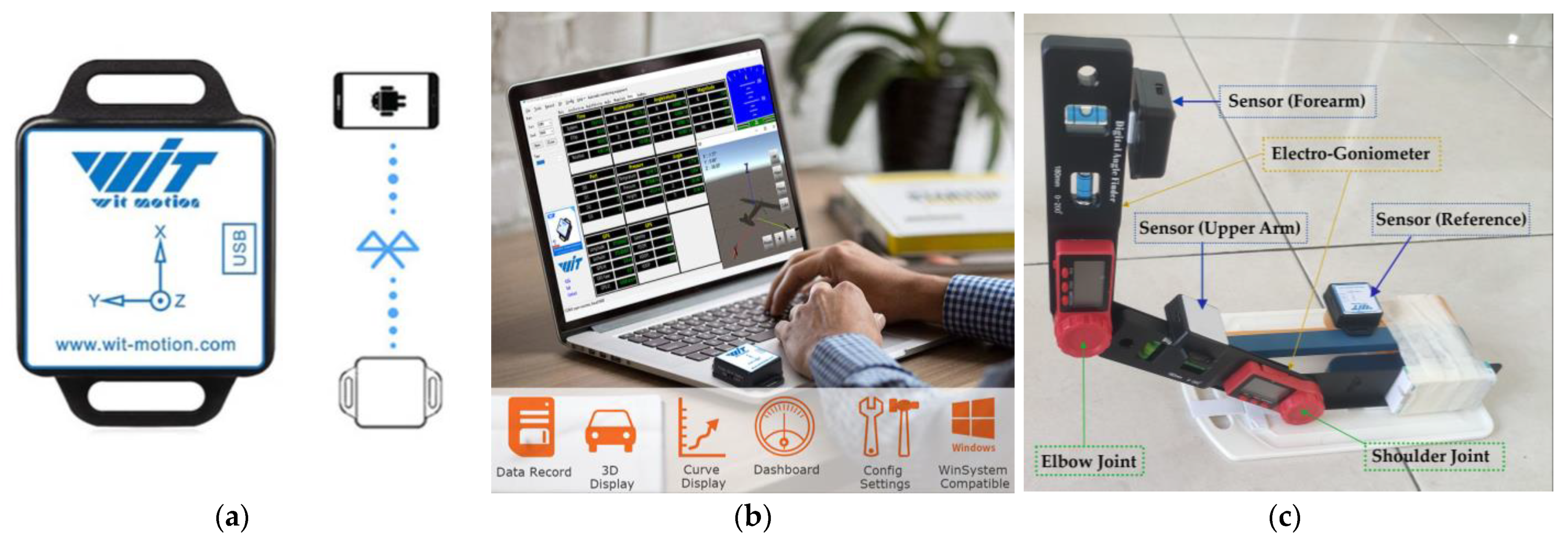
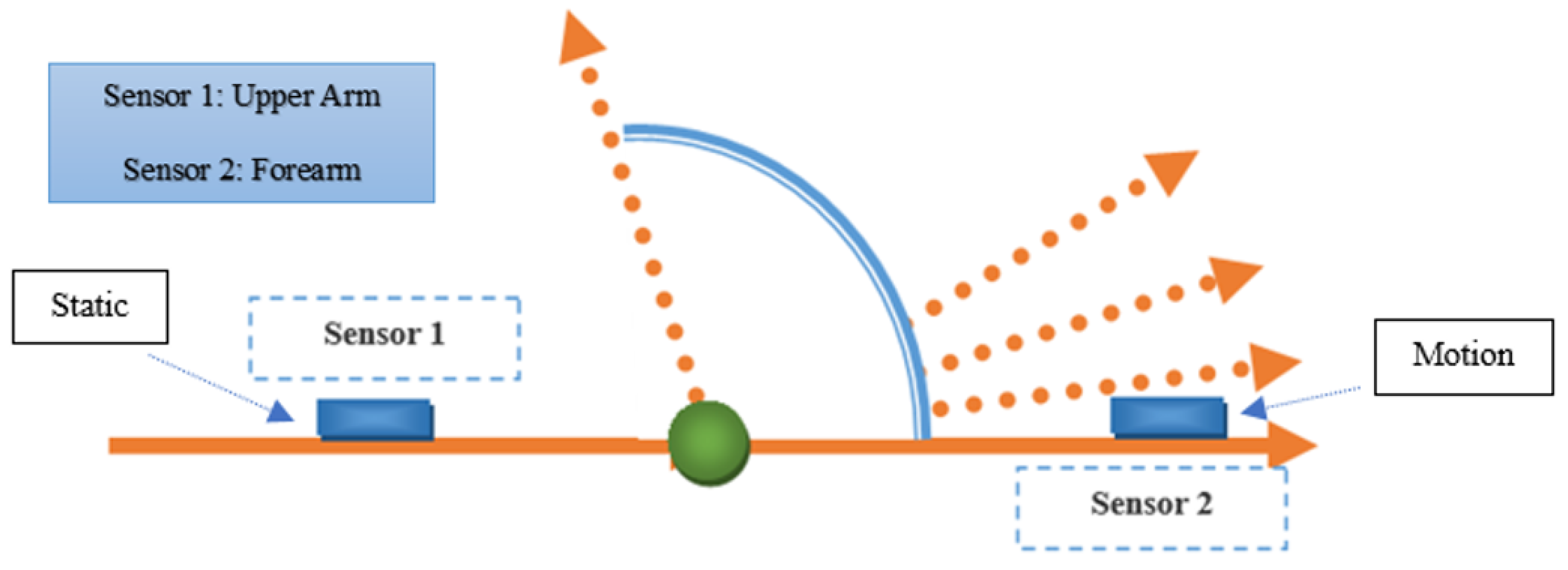
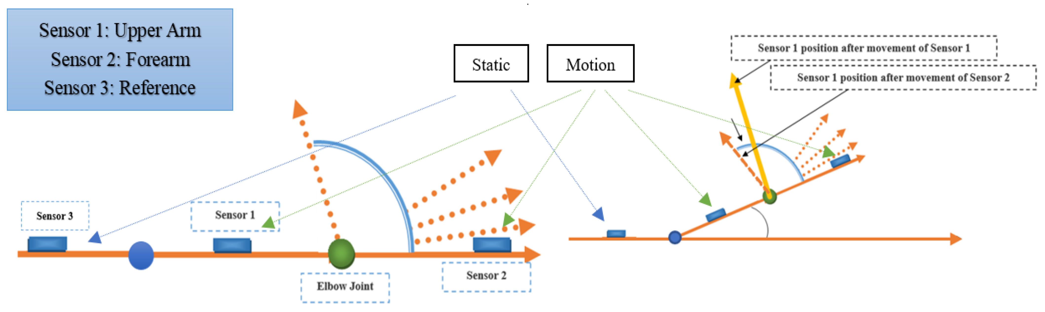
2.1. Experimental Scenario and Platform

This system comprised three wireless sensor nodes, each of which was equipped with a relatively inexpensive MEMS inertial sensor MPU9250. This MPU9250 is a low-cost 9-axis MEMS IMU made by WitMotion Company. The inertial sensor comprises a gyroscope with three axes, an accelerometer with three axes, and a magnetometer with three axes. The dimensions of the inertial sensor are 51.3 mm × 36 mm × 15 mm, and the net weight is 20 g.

Table 1. IMU specifications. Source: https://www.wit-motion.com/. Accessed on 5 September 2022.

Parameter	Technical Specification
Dimension	51.3 mm × 36 mm × 15 mm
Net Weight	20 g
Chip	nRF52832 Bluetooth chip
Processor	Cortex-M0 core processor
IMU	MPU9250
Voltage	3.3–5 V
Output	3-axis Acceleration + Angle + Angular Velocity + Magnetic Field + Quaternion
Range	Acceleration (±16 g), Gyroscope (±2000°/s), Magnet Field (±4900 µT)
Angle Accuracy	X, Y-axis: 0.05° (Static) X, Y-axis: 0.1° (Dynamic)

provides a comprehensive summary of the IMU’s numerous features and parameters.

Figure 1a,b depicts the hardware configuration of the inertial motion capture system used in this study. BLE 5.0 multiple connection software was utilized to link a PC with IMU sensors, which has a 50 m coverage range (without obstacles like walls). This software can retrieve and save CSV files containing data from accelerometers, gyroscopes, and magnetometers.

The elbow joint angle of the human body was represented by a 3D rigid body, shown in Figure 1c, which resembles an arm of the human body. The rigid body was designed and developed utilizing two electro-goniometers that were joined together using a strong adhesive, as shown in Figure 1c. The electro-goniometers have an accuracy of 0.5° with a measuring range of 0–200°. This structure was then placed on a platform to develop a complete arrangement. This rigid body has three segments or arms. One arm represents the upper arm, the second arm represents the forearm, and the third arm represents the shoulder part of the human body. Sensors were attached to each arm of the rigid body and raw sensor data were collected at a rate of 10 samples per second. These IMU sensor data were used to determine the elbow joint angle of the rigid body during static and dynamic conditions.

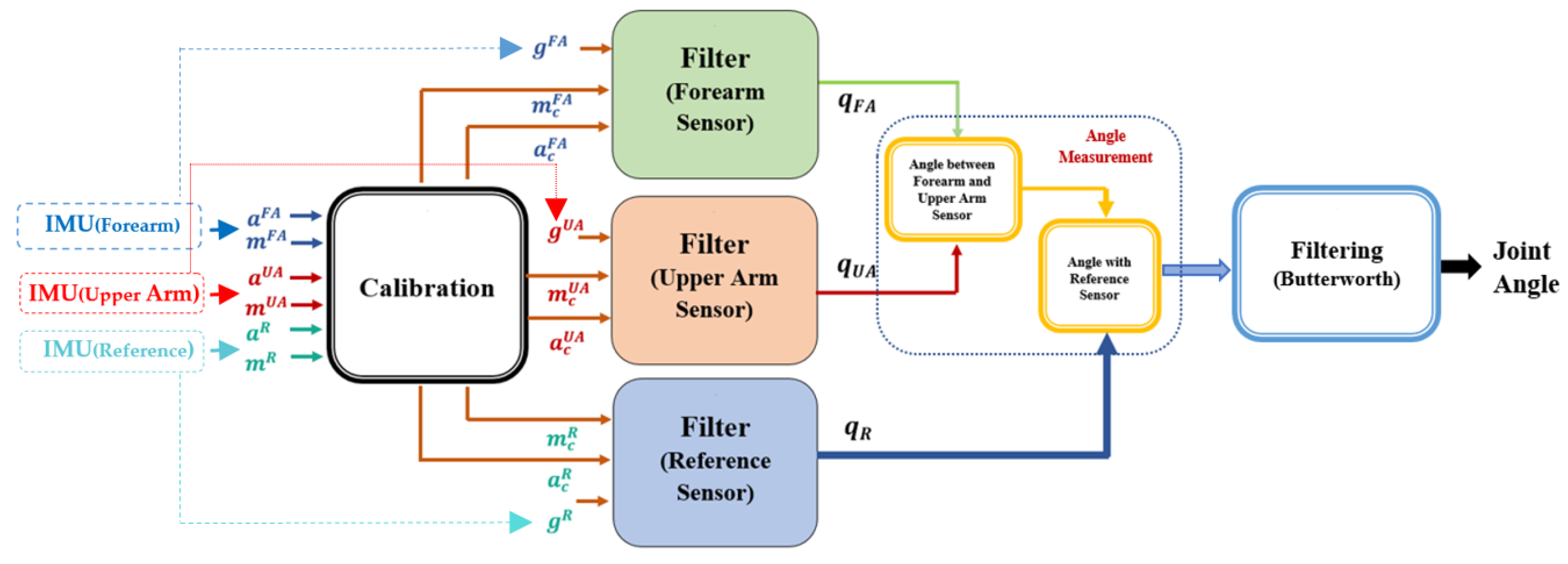
2.2. Joint Angle Measurement Algorithm

In this study, we proposed a two-stage orientation measurement algorithm that can estimate the joint angles of the elbow joint using the accelerometer, gyroscope, and magnetometer raw data from three IMUs. Among them, two IMUs were attached above and below the elbow joint of the rigid body, and the third IMU acted as a reference, placed in the shoulder position (static). At the beginning of the proposed algorithm, each IMU sensor’s data were calibrated, and in the first stage, all sensor data were fused using the Madgwick filter, which returns output in quaternion form. In the second stage, the joint angle was estimated by fusing the quaternion data of all IMUs obtained in the first stage. Finally, to eliminate the high frequency components from the estimated angle, the joint angle was passed through a fourth-order Butterworth low-pass filter. Algorithm 1 outlines the procedure that has been proposed for estimating the joint angle. The proposed algorithm is represented as a block diagram in Figure 2.

Algorithm 1 Proposed Joint Angle Measurement Algorithm

1  Initialization and calibration of the forearm, upper arm, and reference sensor:    Accelerometer data: $a^i$    Gyroscope data: $g^i$    Magnetometer data: $m^i$ 2  Collection of Accelerometer, Gyroscope, and Magnetometer raw data 3  Measurement of bias correction vector ($b_i$) from acceleration data 4  Calibration of Accelerometer data using bias correction vector: $$a_c^k=\left(a^k-b_i\right)$$ 5  Conversion of Magnetometer data ($m^i$) from local frame to global frame 6  Calibration and correction of the Magnetometer data in global frame: $$m_c^k=\left[q_b q_c q_d\right]$$ 7  First Stage: Use of Madgwick filter for all three sensors‘ orientation estimation Output: Forearm Sensor $\to q_{FA}$ Upper Arm Sensor $\to q_{UA}$ Reference Sensor $\to q_R$ 8  Second Stage: Calculation of Joint Angle (θ) from the three quaternions 9  Filtering of Joint Angle ($\theta$) using Fourth-Order Butterworth Filter

2.2.1. Calibration

When an IMU is at rest, the accelerometer should only measure gravity, and the gyroscope should show zero rotational velocity. In contrast, they always show some data while still in real-world circumstances. On the other hand, the magnetometer has issues with magnetic interference [21]. To minimize these issues, calibration was therefore required for the magnetometer, gyroscope, and accelerometer. With the aid of WitMotion’s built-in software, each of the three sensors—accelerometer, gyroscope, and magnetometer—were calibrated. Gyroscope calibration was sufficient using WitMotion software, but the accelerometer and magnetometer required more than this procedure. In light of this, further calibration of these two sensors was essential, and an additional simple calibration was performed as an early step in the algorithm to reduce or eliminate the bias in data after performing calibration using the manufacturer software. If the sensor was not calibrated using this two-stage algorithm, the results would be different from the actual value.

This calibration process and the calculation are simple, less time-consuming, and easy to follow. Thus, this extra process did not increase the calculation burden.

Table 2. Inertial sensor calibration shortcomings mentioned in the previous literature and advantages of the proposed calibration process.

Ref.	Year	Shortcomings of Calibration Process (Previous Literature)	Advantages of Proposed Calibration Process
[14]	2022	Cumbersome calibration procedure	The procedure and calculation are simple Requires small dataset Positioning the sensor for calibration purposes is straightforward, and rotation of the sensor is not required The process is not time consuming Each sensor calibration process is independent
[37]	2022	Deep convolutional neural network Calib-Net was implemented, where internal algorithms are more difficult to interpret from a physical and geometric perspective
[38]	2020	A total of thirty positions are needed for the process, which is a laborious task
[39]	2020	Training necessitates a substantial dataset at the beginning
[40]	2017	Numerical integration could result in inaccuracies
[41]	2017	Difficult procedure Inconvenient for engineering application
[42]	2015	Gyroscope precision is dependent on the calibration accuracy of the accelerometer

depicts the shortcomings of various calibration techniques described in other research articles and the advantages of this proposed calibration process over the previous research.

The acceleration ($a^i$), angular velocity ($g^i$), and magnetic field strength ($m^i$) of the IMU about the x, y, and z axes were measured with a tri-axis accelerometer, gyroscope, and magnetometer, and they were expressed as

$$a^i=\left[a_{xi}\hspace{1em}{a}_{yi}\hspace{1em}{a}_{zi}\right]$$

(1)

$$g^i=\left[{\omega }_{xi}\hspace{1em}{\omega }_{yi}\hspace{1em}{\omega }_{zi}\right]$$

(2)

$$m^i=\left[m_{xi}\hspace{1em}{m}_{yi}\hspace{1em}{m}_{zi}\right]$$

(3)

where i = 1 (for forearm sensor), 2 (for upper arm sensor), 3 (for reference sensor).

In this system, the accelerometer was calibrated using the bias correction vector. During the measurement, the sensors were in static condition for at least 10 s. The first hundred raw accelerometer data were used for determining the bias correction vector for the calibration of the accelerometer. The bias correction vector and calibrated value of the accelerometer were calculated from Equations (4) and (5), respectively.

$$b_i=\left[\frac{{{\displaystyle \sum }}_0^{100}\left(a_{x{i}_{bias}}\right)}{100}\hspace{1em}\frac{{{\displaystyle \sum }}_0^{100}\left(a_{y{i}_{bias}}\right)}{100}\hspace{1em}\frac{{{\displaystyle \sum }}_0^{100}\left(a_{z{i}_{bias}}\right)}{100}\right]$$

(4)

$$a_c^k=\left(a^k-b_i\right)$$

(5)

where

$b_i=$ bias in accelerometer readings;

$a^k=$ accelerometer reading after calibration by WitMotion software;

$a_c^k=$ calibrated accelerometer data.

When there was a value of roll and pitch, the magnetometer data in the local coordinate system were transferred to the global coordinate system. This transformation was performed using Equations (6)–(8), where $m_{Gx}$,$m_{Gy}$, and $m_{Gz}$ are the magnetometer measurements in the global coordinate frame in X, Y, and Z axes.

$$m_{Gx}=m_{xi}\cos \theta +m_{yi}\sin \theta \sin \phi +m_{zi}\sin \theta \cos \phi$$

(6)

$$m_{Gy}=m_{yi}\cos \phi -m_{zi}\sin \phi$$

(7)

$$m_{Gz}=-m_{xi}\sin \theta +m_{yi}\sin \phi \cos \theta +m_{zi}\cos \phi \cos \theta$$

(8)

The yaw angle, calculated using Equations (6)–(8), is the heading of the sensor with respect to the magnetic north. However, the magnetometer data were converted to get the initial zero yaw angle using Equations (9)–(14).

$$m_{i\left(avg\right)}=\left[m_{x{i}_{avg}}\hspace{1em}{m}_{y{i}_{avg}}\hspace{1em}{m}_{z{i}_{avg}}\right]=\left[\frac{{{\displaystyle \sum }}_0^{100}\left(m_{x{i}_j}\right)}{100}\hspace{1em}\frac{{{\displaystyle \sum }}_0^{100}\left(m_{y{i}_j}\right)}{100}\hspace{1em}\frac{{{\displaystyle \sum }}_0^{100}\left(m_{z{i}_j}\right)}{100}\right]$$

(9)

$$heading=\left[0\hspace{1em}0\hspace{1em}Atan2\left(m_{y{i}_{avg}},m_{x{i}_{avg}}\right)\right]$$

(10)

$$q_h=\left[q_{h0}\hspace{1em}{q}_{h1}\hspace{1em}{q}_{h2}\hspace{1em}{q}_{h3}\right]$$

(11)

$$q_{m_k}=\left[0\hspace{1em}{m}_{Gx}\hspace{1em}{m}_{Gy}\hspace{1em}{m}_{Gz}\right]$$

(12)

$$q_{m_c^k}=\left(q_h\otimes q_{m_k}\right)\otimes q_h^{*}=\left[q_a\hspace{1em}{q}_b\hspace{1em}{q}_c\hspace{1em}{q}_d\right]$$

(13)

$$m_c^k=\left[q_b\hspace{1em}{q}_c\hspace{1em}{q}_d\right]$$

(14)

where

$m_{i\left(avg\right)}=$ average of first hundred data of magnetometer along X, Y, and Z axes;

$q_h=$ quaternion corresponding to the heading angle;

$q_{m_c^k}=$ quaternion corresponding to the corrected magnetometer data;

$m_c^k=$ corrected magnetometer data.

2.2.2. First Stage: Estimation of Orientation from Sensor Fusion Technique

The Madgwick algorithm (MAD) was implemented in this study as an orientation filter. The MAD is a sensor fusion algorithm that combines the data from the accelerometer, gyroscope, and magnetometer in a quaternion form. This algorithm computes a quaternion derivative of the IMU, which can be converted to Euler angles. Although the sample rate restricts the range of the motion or joint angle measurement accuracy, satisfactory behavior was recorded even when utilizing low sampling rates, close to 10 Hz, and this level of accuracy may be suitable for applications involving human motion [32]. The Madgwick filter is an algorithm based on gradient descent that can compensate gyroscope drift [32]. The advantages of the Madgwick filter are its low computational load and complexity, low sampling rate requirement, that it can compensate for magnetic distortion, and that it has a simple tuning method where there is only one adjustable parameter. Since MAD uses a quaternion representation, the filter is not subjected to the gimbal lock problem associated with Euler angle representation. The Madgwick algorithm is also very convenient for small-size, low-cost, and low-energy-consumption microprocessors.

The implementation of the proposed algorithm was carried out with the assistance of Matlab R2022a. After going through the calibration steps, the data from three IMUs (forearm, upper arm, and reference) acted as an input for the Madgwick filter. The filter’s output was three different sets of quaternions for the upper arm, forearm, and reference sensors. These three sets of quaternions were utilized to compute the joint angle of the rigid body. The Madgwick filter’s precise details are stated in Algorithm 2.

Algorithm 2 Madgwick Filter [32]

First Step: Computation of the orientation from the gyroscope. Gyroscope measurement: ${\mathit{S}}_{\mathsf{\omega }}=\mathbf{\left[}\mathbf{0} {\mathsf{\omega }}_{\mathit{x}} {\mathsf{\omega }}_{\mathit{y}} {\mathsf{\omega }}_{\mathit{z}}\mathbf{\right]}$ Quaternion derivative: ${}_{ \mathit{E}}{}^{\mathit{S}}\dot{\mathit{q}}{}_{\mathit{w}\mathbf{,}\mathit{t}}=\frac{\mathbf{1}}{\mathbf{2}}{}_{\mathit{E}}{}^{\mathit{S}}\widehat{\mathit{q}}{}_{\mathit{e}\mathit{s}\mathit{t}\mathbf{,}\mathit{t}-\mathbf{1}}\mathbf{\otimes } {\mathit{S}}_{\mathsf{\omega }}{}_{\mathit{t}}$ Orientation from Gyroscope, ${}_{\mathit{E}}{}^{\mathit{S}}\mathit{q}{}_{\mathsf{\omega }\mathbf{,}\mathit{t}}=\frac{\mathbf{1}}{\mathbf{2}}{}_{\mathit{E}}{}^{\mathit{S}}\widehat{\mathit{q}}{}_{\mathit{e}\mathit{s}\mathit{t}\mathbf{,}\mathit{t}-\mathbf{1}}+ {}_{ \mathit{E}}{}^{\mathit{S}}\dot{\mathit{q}}{}_{\mathit{w}\mathbf{,}\mathit{t}}\mathbf{\Delta }\mathit{t}$ Second Step: Use of accelerometer data to get the orientation quaternion. Sensor Orientation: ${}_{\mathit{E}}{}^{\mathit{S}}\widehat{\mathit{q}}=\mathbf{\left[}{\mathit{q}}_{\mathbf{1}} {\mathit{q}}_{\mathbf{2}} {\mathit{q}}_{\mathbf{3}} {\mathit{q}}_{\mathbf{4}}\mathbf{\right]}$ Predefined reference direction of the field in the earth frame: $${\mathit{E}}_{\widehat{\mathit{d}}}=\mathbf{\left[}\mathbf{0} {\mathit{d}}_{\mathit{x}} {\mathit{d}}_{\mathit{y}} {\mathit{d}}_{\mathit{z}}\mathbf{\right]}$$ Measurement of the field in the sensor frame, ${\mathit{S}}_{\widehat{\mathit{S}}}=\mathbf{\left[}\mathbf{0} {\mathit{s}}_{\mathit{x}} {\mathit{s}}_{\mathit{y}} {\mathit{s}}_{\mathit{z}}\mathbf{\right]}$ The sensor orientation ${}_{\mathit{E}}{}^{\mathit{S}}\widehat{\mathit{q}}$ can be formulated as an optimization problem by $$\underset{{}_{\mathit{E}}{}^{\mathit{S}}\widehat{\mathit{q}} \mathbf{\in }{\mathit{R}}^{\mathbf{4}}}{\mathbf{min}}\mathit{f}\mathbf{\left(}{}_{\mathit{E}}{}^{\mathit{S}}\widehat{\mathit{q}}\mathbf{,}{\mathit{E}}_{\widehat{\mathit{d}}}\mathbf{,}{\mathit{S}}_{\widehat{\mathit{S}}}\mathbf{\right)}$$ where the objective function $\mathit{f}\mathbf{\left(}{}_{\mathit{E}}{}^{\mathit{S}}\widehat{\mathit{q}}\mathbf{,}{\mathit{E}}_{\widehat{\mathit{d}}}\mathbf{,}{\mathit{S}}_{\widehat{\mathit{S}}}\mathbf{\right)}$ can be calculated by $$\mathbf{(}{}_{\mathit{E}}{}^{\mathsf{S}}\widehat{\mathit{q}}{}^{\mathbf{*}}\mathbf{\otimes }{\mathit{E}}_{\widehat{\mathit{d}}}\mathbf{\otimes }{}_{\mathit{E}}{}^{\mathsf{S}}\widehat{\mathit{q}}-{\mathit{S}}_{\widehat{\mathit{S}}}\mathbf{)}$$ Using Gradient Descent algorithm, estimated orientation based on previous one and $\mathsf{\mu }$ step size:   $${}_{\mathit{E}}{}^{\mathit{S}}\widehat{\mathit{q}}{}_{\mathit{k}+\mathbf{1}}={}_{\mathit{E}}{}^{\mathit{S}}\widehat{\mathit{q}}{}_{\mathit{k}}-\mathsf{\mu }\frac{\mathsf{\nabla }\mathit{f}\mathbf{\left(}{}_{\mathit{E}}{}^{\mathit{S}}\widehat{\mathit{q}}\mathbf{,}{\mathit{E}}_{\widehat{\mathit{d}}}\mathbf{,}{\mathit{S}}_{\widehat{\mathit{S}}}\mathbf{\right)}}{\Vert \mathsf{\nabla }\mathit{f}\mathbf{\left(}{}_{\mathit{E}}{}^{\mathit{S}}\widehat{\mathit{q}}\mathbf{,}{\mathbf{E}}_{\widehat{\mathit{d}}}\mathbf{,}{\mathit{S}}_{\widehat{\mathit{S}}}\mathbf{\right)}\Vert }$$ where $\mathsf{\nabla }\mathit{f}\mathbf{\left(}{}_{\mathit{E}}{}^{\mathit{S}}\widehat{\mathit{q}}\mathbf{,}{\mathit{E}}_{\widehat{\mathit{d}}}\mathbf{,}{\mathit{S}}_{\widehat{\mathit{S}}}\mathbf{\right)}={\mathit{J}}^{\mathit{T}}\mathbf{\left(}{}_{\mathit{E}}{}^{\mathit{S}}\widehat{\mathit{q}}{}_{\mathit{k}}\mathbf{,}{\mathit{E}}_{\widehat{\mathit{d}}}\mathbf{\right)} \mathit{f}\mathbf{\left(}{}_{\mathit{E}}{}^{\mathit{S}}\widehat{\mathit{q}}\mathbf{,}{\mathit{E}}_{\widehat{\mathit{d}}}\mathbf{,}{\mathit{S}}_{\widehat{\mathit{S}}}\mathbf{\right)}$ For accelerometer, the Objective function and the Jacobian matrix are ${\mathit{f}}_{\mathit{g}}\mathbf{\left(}{}_{\mathit{E}}{}^{\mathit{S}}\widehat{\mathit{q}}\mathbf{,}{\mathit{S}}_{\widehat{\mathit{a}}}\mathbf{\right)}$ and ${\mathit{J}}_{\mathit{g}}\mathbf{\left(}{}_{\mathit{E}}{}^{\mathit{S}}\widehat{\mathit{q}}\mathbf{\right)}$. Third Step: Use of magnetometer data. Earth’s magnetic field: ${\mathit{E}}_{\widehat{\mathit{b}}}=\mathbf{\left[}\mathbf{0} {\mathit{b}}_{\mathit{x}} \mathbf{0} {\mathit{b}}_{\mathit{z}}\mathbf{\right]}$ Magnetometer measurement: ${\mathit{S}}_{\widehat{\mathit{m}}}=\mathbf{\left[}\mathbf{0} {\mathit{m}}_{\mathit{x}} {\mathit{m}}_{\mathit{y}} {\mathit{m}}_{\mathit{z}}\mathbf{\right]}$ For Magnetometer the Objective function and the Jacobian matrix are ${\mathit{f}}_{\mathit{b}}\mathbf{\left(}{}_{\mathit{E}}{}^{\mathit{S}}\widehat{\mathit{q}}\mathbf{,}{\mathit{E}}_{\widehat{\mathit{b}}}\mathbf{,}{\mathit{S}}_{\widehat{\mathit{m}}}\mathbf{\right)}$ and ${\mathit{J}}_{\mathit{b}}\mathbf{\left(}{}_{\mathit{E}}{}^{\mathit{S}}\widehat{\mathit{q}}\mathbf{,}{\mathit{E}}_{\widehat{\mathit{b}}}\mathbf{\right)}$ respectively. Complete solution considering accelerometer and magnetometer: Objective function: ${\mathit{f}}_{\mathit{g}\mathbf{,}\mathit{b}}\mathbf{\left(}{}_{\mathit{E}}{}^{\mathit{S}}\widehat{\mathit{q}}\mathbf{,}{\mathit{S}}_{\mathit{a}}\mathbf{,} {\mathit{E}}_{\widehat{\mathit{b}}}\mathbf{,}{\mathit{S}}_{\widehat{\mathit{m}}}\mathbf{\right)}=\mathbf{\left(}\begin{array}{c}{\mathit{f}}_{\mathit{g}}\mathbf{\left(}{}_{\mathit{E}}{}^{\mathit{S}}\widehat{\mathit{q}}\mathbf{,}{\mathit{S}}_{\widehat{\mathit{a}}}\mathbf{\right)}\\ {\mathit{f}}_{\mathit{b}}\mathbf{\left(}{}_{\mathit{E}}{}^{\mathit{S}}\widehat{\mathit{q}}\mathbf{,}{\mathit{E}}_{\widehat{\mathit{b}}}\mathbf{,}{\mathit{S}}_{\widehat{\mathit{m}}}\mathbf{\right)}\end{array}\mathbf{\right)}$ Jacobian matrix: ${\mathit{J}}_{\mathit{g}\mathbf{,}\mathit{b}}\mathbf{\left(}{}_{\mathit{E}}{}^{\mathit{S}}\widehat{\mathit{q}}\mathbf{,}{\mathit{E}}_{\widehat{\mathit{b}}}\mathbf{\right)}$ = $\mathbf{\left(}\begin{array}{c}{\mathit{J}}_{\mathit{g}}\mathbf{\left(}{}_{\mathit{E}}{}^{\mathit{S}}\widehat{\mathit{q}}\mathbf{\right)}\\ {\mathit{J}}_{\mathit{b}}\mathbf{\left(}{}_{\mathit{E}}{}^{\mathit{S}}\widehat{\mathit{q}}\mathbf{,}{\mathit{E}}_{\widehat{\mathit{b}}}\mathbf{\right)}\end{array}\mathbf{\right)}$  Estimated Orientation, ${}_{\mathit{E}}{}^{\mathit{S}}\mathit{q}{}_{\mathsf{\nabla }\mathbf{,}\mathit{t}}=$ $\frac{\mathbf{1}}{\mathbf{2}}{}_{\mathit{E}}{}^{\mathit{S}}\mathit{q}{}_{\mathit{e}\mathit{s}\mathit{t}\mathbf{,}\mathit{t}-\mathbf{1}}-\mathsf{\mu } \frac{\mathsf{\nabla }\mathit{f}}{\Vert \mathsf{\nabla }\mathit{f}\Vert }$  where, $\mathsf{\nabla }\mathit{f}$ = ${\mathit{J}}^{\mathit{T}}{}_{\mathit{g}\mathbf{,}\mathit{b}}\mathbf{\left(}{}_{\mathit{E}}{}^{\mathit{S}}\widehat{\mathit{q}}\mathbf{,}{\mathit{E}}_{\widehat{\mathit{b}}}\mathbf{\right)}{\mathit{f}}_{\mathit{g}\mathbf{,}\mathit{b}}\mathbf{\left(}{}_{\mathit{E}}{}^{\mathit{S}}\widehat{\mathit{q}}\mathbf{,}{\mathit{S}}_{\mathit{a}}\mathbf{,} {\mathit{E}}_{\widehat{\mathit{b}}}\mathbf{,}{\mathit{S}}_{\widehat{\mathit{m}}}\mathbf{\right)}$ and $\mathsf{\mu }=\mathsf{\alpha }{}_{ \mathit{E}}{}^{\mathit{S}}\dot{\mathit{q}}{}_{\mathit{w}\mathbf{,}\mathit{t}}\mathbf{\Delta }\mathit{t} \mathbf{,} \alpha \mathbf{>}\mathbf{1}$ Final Step: Final estimation of the orientation:  $${}_{\mathit{E}}{}^{\mathit{S}}\mathit{q}{}_{\mathit{e}\mathit{s}\mathit{t}\mathbf{,}\mathit{t}}=\mathsf{\gamma }\mathit{t}{}_{\mathit{E}}{}^{\mathit{S}}\mathit{q}{}_{\mathsf{\nabla }\mathbf{,}\mathit{t}}+\mathbf{\left(}\mathbf{1}-\mathsf{\gamma }\mathbf{\right)}{}_{\mathit{E}}{}^{\mathit{S}}\mathit{q}{}_{\mathsf{\omega }\mathbf{,}\mathit{t}}$$ The simple expression after some simplifications and assumptions:   $${}_{\mathit{E}}{}^{\mathit{S}}\mathit{q}{}_{\mathit{e}\mathit{s}\mathit{t}\mathbf{,}\mathit{t}}=-\mathsf{\beta } \frac{\mathsf{\nabla }\mathit{f}}{\Vert \mathsf{\nabla }\mathit{f}\Vert }\mathbf{\Delta }\mathit{t}+{}_{\mathit{E}}{}^{\mathit{S}}\widehat{\mathit{q}}{}_{\mathit{e}\mathit{s}\mathit{t}\mathbf{,}\mathit{t}-\mathbf{1}}+{}_{\mathit{E}}{}^{\mathit{S}}\dot{\mathit{q}}{}_{w\mathbf{,}\mathit{t}}\mathbf{\Delta }\mathit{t}$$

2.2.3. Second Stage: Measurement of Angle

The quaternions for the forearm, upper arm, and reference from the first stage were denoted by $q_{FA}$, $q_{UA},$ and $q_R,$ respectively.

$$q_{FA}=\left[q_{F0}\hspace{1em}{q}_{F1}\hspace{1em}{q}_{F2}\hspace{1em}{q}_{F3}\right]$$

(15)

$$q_{UA}=\left[q_{U0}\hspace{1em}{q}_{U1}\hspace{1em}{q}_{U2}\hspace{1em}{q}_{U3}\right]$$

(16)

$$q_R=\left[q_{R0}\hspace{1em}{q}_{R1}\hspace{1em}{q}_{R2}\hspace{1em}{q}_{R3}\right]$$

(17)

If the upper arm is completely static, it is possible to calculate the joint angle from the initial and final quaternion of the forearm sensor. However, as the upper arm sensor may move with the movement of the forearm, the actual angle between the upper arm and forearm can be found by using the quaternion of two sensors placed on the forearm and upper arm. Considering this, the quaternion corresponding to the angle (${\theta }_1$) between these two sensors was found using Equation (18).

$$q_{UF}=q_{UA}\times q_{FA}^{*}=\left[q_{UF0} q_{UF1} q_{UF2} q_{UF3}\right]$$

(18)

The angle (${\theta }_1$) between the forearm and upper arm sensors was obtained from the quaternion $q_{UF}$ using Equation (19).

$$\mathrm{Angle} \left({\theta }_1\right)=\left[Atan2\left(\left(1-\left(q_{\mathrm{UF}2}^2+q_{\mathrm{UF}3}^2\right)\right),2\left(q_{\mathrm{UF}0}{q}_{\mathrm{UF}3}+q_{\mathrm{UF}1}{q}_{\mathrm{UF}2}\right)\right)\right]\times 57.3$$

(19)

Moreover, the impact of the movement of the upper arm could be found by using Equation (20).

$$q_{UFR}=q_{UF}\times q_R^{*}=\left[q_0\hspace{1em}{q}_1\hspace{1em}{q}_2\hspace{1em}{q}_3\right]$$

(20)

The more precise joint angle (${\theta }_2$) was obtained from the quaternion $q_{UFR}$ using Equation (21).

$$\mathrm{Joint}\mathrm{Angle}, {\theta }_2=\left[Atan2\left(\left(1-\left(q_2^2+q_3^2\right)\right),2\left(q_0{q}_3+q_1{q}_2\right)\right)\right]\times 57.3$$

(21)

2.2.4. Filtering

An accelerometer can accurately calculate roll and pitch angles for a stationary object on Earth. If the sensor moves, acceleration will alter rotation computation. Additionally, the adjacent magnetic fields’ impact causes the magnetometer’s results to be inaccurate. Therefore, filtering is quite important, and this particular design filters the final angle. The data filtering process was carried out using a fourth-order Butterworth filter.

3. Results and Discussion

The effectiveness of the proposed algorithm is evaluated and discussed in this section.

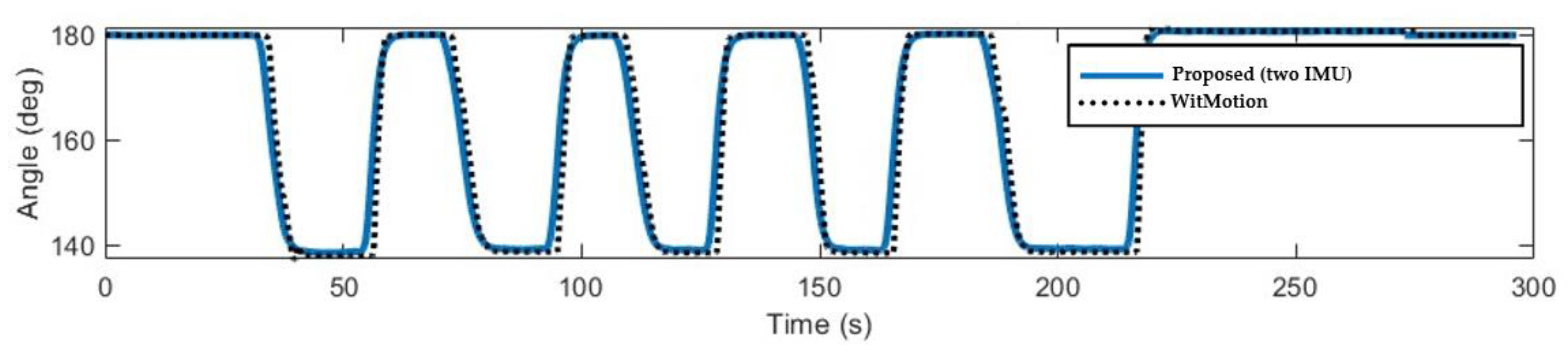
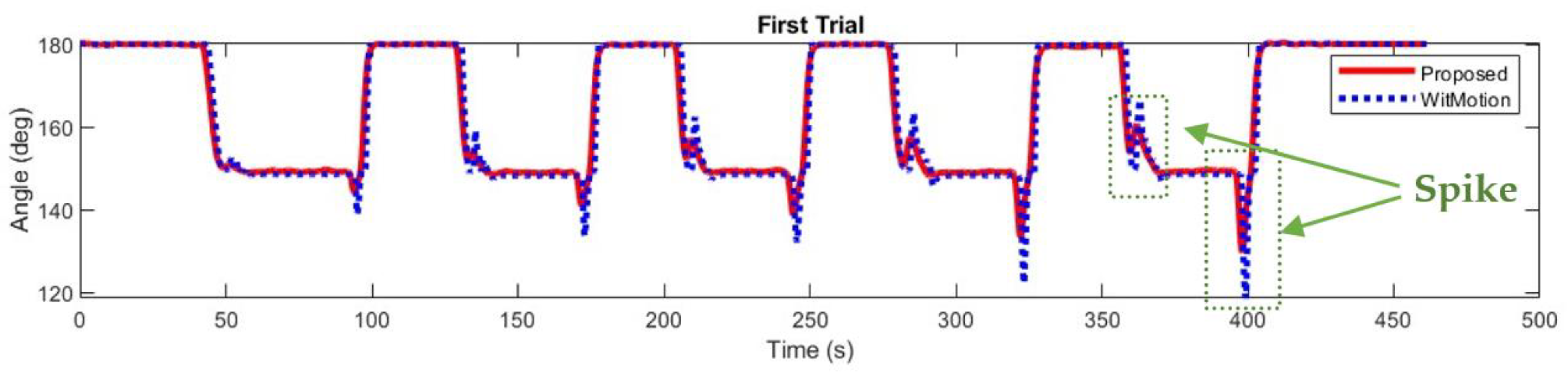
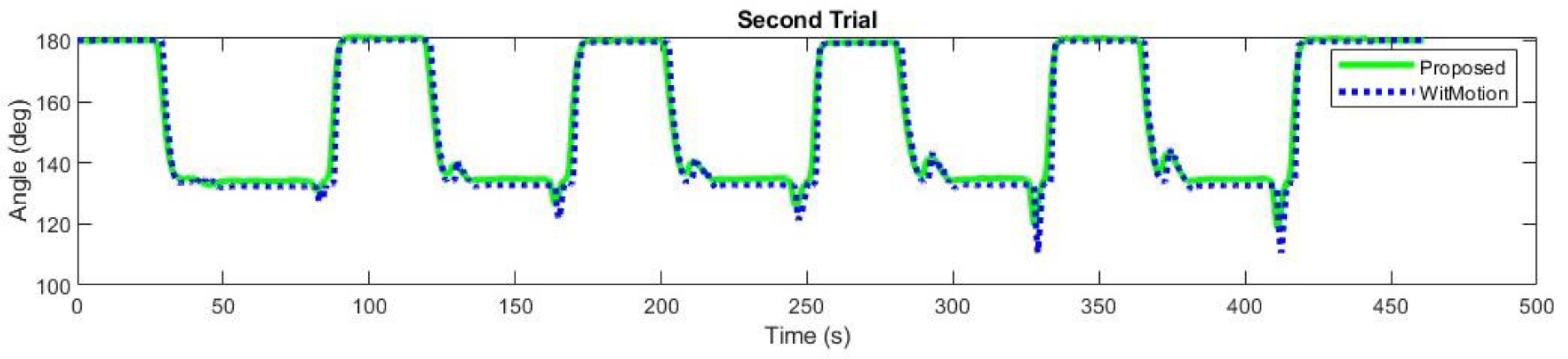
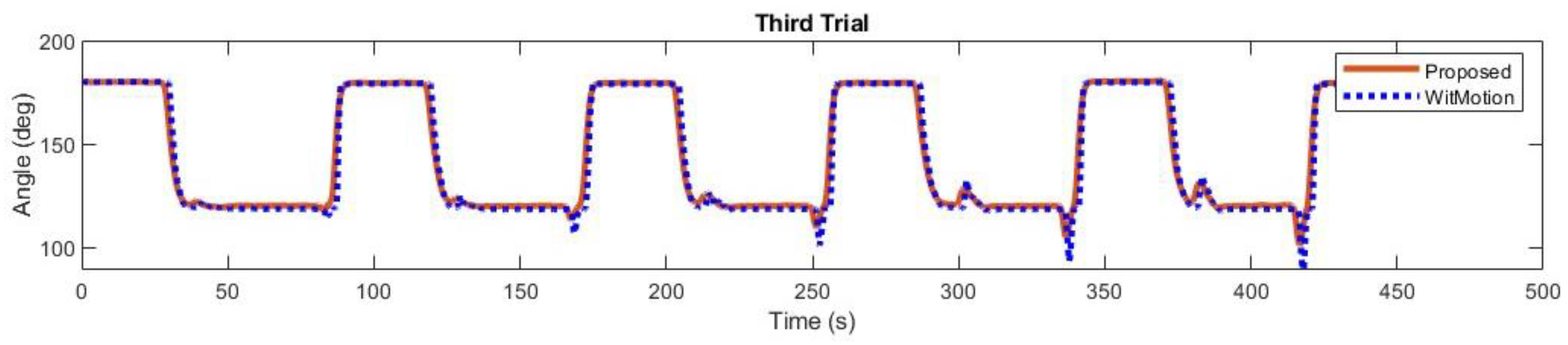
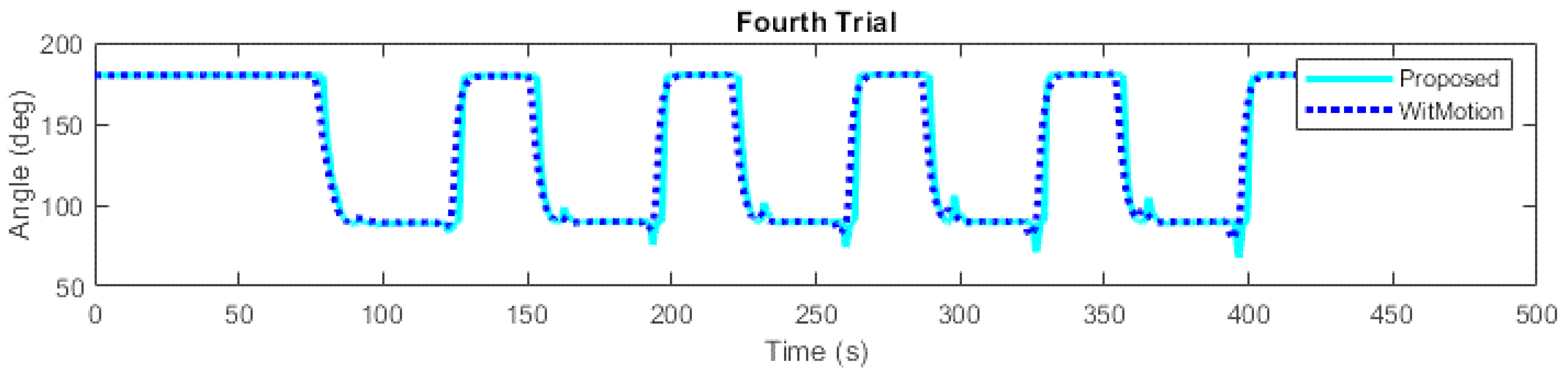
3.1. Joint Angle Measurement

The performance of the proposed joint monitoring algorithm was first tested to obtain the elbow joint angle of the rigid body using two sensors, one in the forearm and another in the upper arm, shown in Figure 3.

The forearm sensor was moved for five consecutive trials, while the upper arm sensor attached to the rigid body was in a static posture. Each time, the forearm was moved around 40°, and the respective joint angle was around 140°. Through the use of the WitMotion software, the raw motion data from the accelerometer, gyroscope, and magnetometer was recorded and gathered. The accelerometer, gyroscope, and magnetometer raw data were collected at 10 samples per second. Following that, the accelerometer and magnetometer sensor data were subjected to a second step of calibration. Then the accelerometer, gyroscope, and magnetometer data were used to calculate quaternion for both sensors, and after that, the joint angle created by the rigid body was calculated using Equation (19). Two electro-goniometers (EGs) were attached with the forearm and the upper arm of the rigid body to measure the joint angle at the same time (shown in Figure 1c) and the angle calculated using the two EGs was considered as the reference value. The WitMotion software itself calculated the orientation of the sensors using the KF. The joint angle from the proposed algorithm (PA) and calculated from the KF outcomes of WitMotion software (WM) for two sensors were compared with the measurement of joint angle from two EGs.

The performance of the proposed algorithm (PA), using two sensors, was evaluated with respect to the angle measurement value of the EGs and the angle measured from the KF outcomes of WitMotion software (WM) in terms of root mean square error (RMSE), which are presented in

Table 3. Angle measurement comparison (RMSE in degrees) between the proposed algorithm (PA) and WitMotion (WM).

EG	PA	WM	Error (PA)	Error (WM)	RMSE (PA)	RMSE (WM)
139.25	139.55	138.86	−0.3	0.39	0.26	0.43
139.5	139.72	139.01	−0.22	0.49
139.2	139.38	138.75	−0.18	0.45
139.65	139.93	139.23	−0.28	0.42
139.2	139.51	138.82	−0.31	0.38

. Figure 4 shows joint angle graphical representations obtained from the proposed algorithm with two sensors and WitMotion outcomes for five different trials. In this case, the RMSEs for PA and WM were 0.26° and 0.43°, respectively. It can be seen that the proposed joint angle measurement system using two sensors and the Madgwick filter gives a more accurate estimation in this case.

In the subsequent case, three sensors were used for more precise measurement of the joint angle between the forearm and the upper arm. The forearm of the body was also moved for four separate trials, where the forearm was moved by approximately 30°, 45°, 60°, and 90° in these four trials, respectively, and the upper arm was moved by 30° in every trial. During the movement of the forearm of the rigid body, shown in Figure 5 (also shown in Figure 1c), the upper arm remained in a stationary position. After the predefined movement of the forearm, the movement of the upper arm was executed. In each trial, the forearm and the upper arm were moved five times, and with the rotation of the upper arm, the final rotation of forearm was shifted to 60°, 75°, 90°, and 120° in the four trials, respectively. Thus, in these trials, the joint angles between the forearm and the upper arm were approximately 150°, 135°, 120°, and 90°.

In each case or trial, the angle between the forearm and upper arm was calculated from the data of the two EGs attached to the forearm and upper arm of the rigid body. The angle calculated with the EGs was considered to be the reference value. Additionally, the raw data from the accelerometer, gyroscope, and magnetometer were collected and used as the input of the proposed algorithm (PA) after executing the calibration process. Three sensors provide three orientations in quaternion form, and using Equations (15)–(21), the more accurate joint angle between the forearm and upper arm was calculated.

In the first trial, at first the forearm was moved by about 30°, and then the upper arm was moved by about 30°. Thus, the angle was approximately 150° between the forearm and upper arm. The angles calculated from the EGs, PA, and WM are presented in

Table 4. RMSE (°) of the joint angle (first trial).

EG	PA	WM	Error (PA)	Error (WM)	RMSE (PA)	RMSE (WM)
149.70	149.32	148.53	−0.38	−1.17	0.46	1.19
149.40	148.91	148.23	−0.49	−1.17
149.65	149.23	148.49	−0.42	−1.16
149.50	148.98	148.29	−0.52	−1.21
149.75	149.27	148.52	−0.48	−1.23

, and Figure 6 shows joint angle graphical representations obtained from the PA and WM for the first trial. In the second trial, the forearm was moved by about 45°, and then the upper arm was moved by about 30°. Thus, the angle was approximately 135° between the forearm and upper arm. The angles calculated from the EGs, PA, and WM are presented in

Table 5. RMSE (°) of the joint angle (second trial).

EG	PA	WM	Error (PA)	Error (WM)	RMSE (PA)	RMSE (WM)
134.05	134.12	132.30	0.07	−1.75	0.10	1.97
134.65	134.76	132.67	0.11	−1.98
134.70	134.83	132.73	0.13	−1.97
134.80	134.93	132.74	0.13	−2.06
134.60	134.65	132.54	0.05	−2.06

, and Figure 7 shows joint angle graphical representations obtained from the PA and WM for the second trial.

In the same way, the outcome of the third and fourth trials is given in

Table 6. RMSE (°) of the joint angle (third trial).

EG	PA	WM	Error (PA)	Error (WM)	RMSE (PA)	RMSE (WM)
120.00	120.19	118.69	0.19	−1.31	0.18	1.40
119.85	120.00	118.48	0.15	−1.37
119.95	120.07	118.58	0.12	−1.37
119.85	119.94	118.35	0.09	−1.50
119.95	120.23	118.50	0.28	−1.45

and

Table 7. RMSE (°) of the joint angle (fourth trial).

EG	PA	WM	Error (PA)	Error (WM)	RMSE (PA)	RMSE (WM)
89.20	89.27	88.89	0.07	−0.31	0.03	0.29
89.95	89.96	89.73	0.01	−0.22
89.90	89.88	89.62	−0.02	−0.28
89.85	89.85	89.59	0.00	−0.26
89.80	89.79	89.42	−0.01	−0.38

, respectively, and graphically represented in Figure 8 and Figure 9, respectively. In the third trial, the forearm was moved by about 60°, and then the upper arm was moved by about 30°. Additionally, in the fourth trial, the forearm was moved by about 90°, and then the upper arm was moved by about 30°.

In these four trials, the RMSEs for the PA and WM were calculated with respect to the joint angle calculated using EGs, and all the results were compared. The calculated RMSEs for the joint angle using the PA were 0.46°, 0.10°, 0.18°, and 0.03°, respectively, and for the WM, the RMSEs were 1.19°, 1.97°, 1.40°, and 0.29°, respectively. The comparison of the RMSE between the PA and WM showed that the proposed joint angle measurement system using the Madgwick filter gave a more accurate estimation for all the trials. Moreover, the RMSE resided within the clinically acceptable threshold of 5° in all cases. There are two spikes during each motion of all the trials, which was only mentioned in Figure 6. This problem was developed as different sensor units’ data alter differently while in motion. The experiments were conducted under the same environmental conditions, and the same posture was used for this experiment.

Table 8. Performance comparison.

Ref.	Year	Structure	Comparison Parameter (RMSE/ Max. Deviation)
[43]	2022	UR3 Robot	RMSE: 1.0029°
[44]	2022	Two links joined by a magnetic encoder	ADXL345 (RMSE) Analytical (3.61° to 11.67°), EKF (3.09° to 7.95°), UKF (3.03° to 7.92°) ADXL357 (RMSE) Analytical (4.7° to 11.39°), EKF (4.8° to 11.42°), UKF (4.8° to 11.37°) BNO055 (RMSE) Analytical (2.99° to 17.72°), EKF (3.47° to 10.52°), UKF (3.45° to 10.51°)
[45]	2022	ROMSS	Max. Deviation: 0.87°
[46]	2021	Artificial joint	Max. Deviation: 0.60°
Proposed Algorithm		3D Rigid body	RMSE: 0.03° to 0.46° Max. Deviation: 0.52°

shows a performance comparison between several existing studies and the proposed algorithm, and for this comparison table, articles only with artificially developed structures were considered.

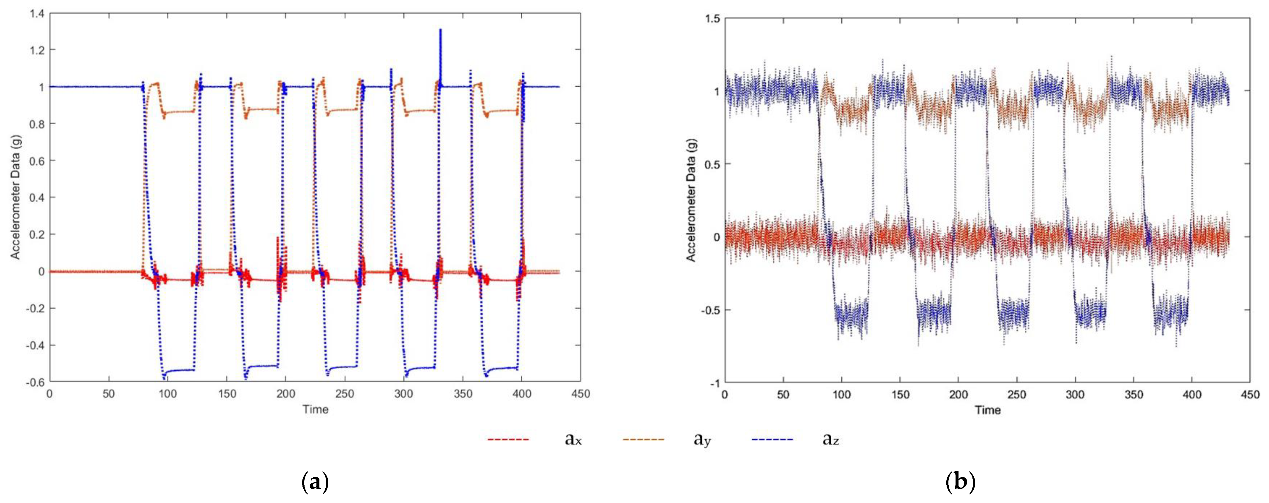
3.2. Joint Angle Measurement Considering External Acceleration

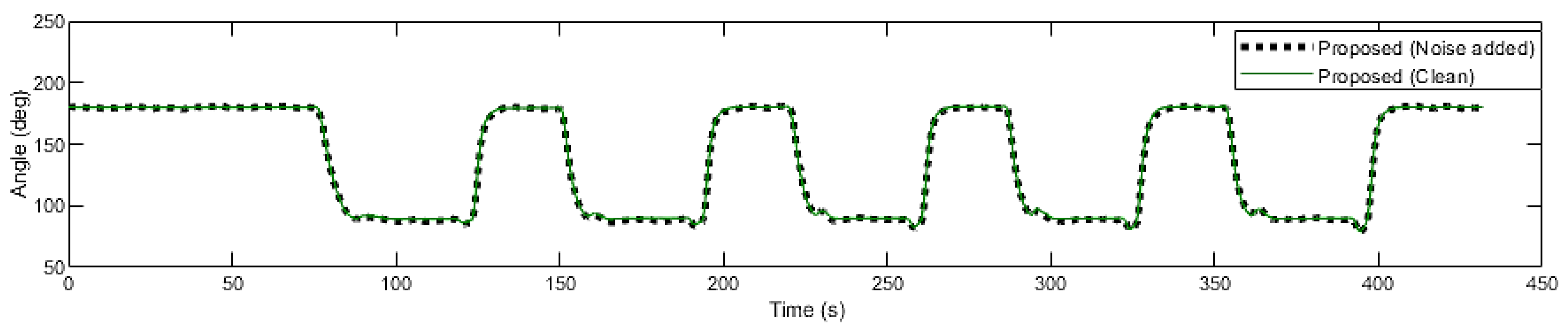
In the presence of an external acceleration, the proposed algorithm’s effectiveness was verified by simulating zero-mean white Gaussian noise to the acceleration measurements of all three IMUs. Zero-mean Gaussian noise was used to create external acceleration as IMU noise is best fitted by a Gaussian distribution, and the noise in IMU is white Gaussian in nature [13,47]. Figure 10a shows the sample raw accelerometer data without external noise, and Figure 10b displays the sample raw accelerometer data with external noise, which was contaminated at 20 dB signal-to-noise ratio (SNR) for one wearable IMU.

In Figure 11, the joint angle is shown, estimated using the proposed algorithm that takes into account the noisy accelerometer data, and compared to the angle obtained using the proposed algorithm with clean accelerometer data.

Table 9. RMSE (°) of the joint angle (external noise added).

EG	PA	Error (PA)	RMSE (PA)
89.20	88.02	1.18	0.996
89.95	88.42	1.53
89.90	89.58	0.32
89.85	88.87	0.98
89.80	89.40	0.40

displays the root mean square error associated with calculated joint angles when an external acceleration is present. Figure 11 and Table 9 both demonstrate that the suggested algorithm was exceptionally resistant to the effects of acceleration from the environment, as the RMSE was 0.996° after the addition of external noise. Moreover, the RMSE value was below the threshold of 5°, which is considered clinically acceptable [13].

3.3. Limitations

In this experiment, the attachment location of the sensors was not precisely regulated, especially the shoulder sensor; nonetheless, while the measurements were being taken, they were aligned approximately in the sagittal plane. The reference sensor may face unwanted motion in real-world scenarios. Thus, this straightforward way of attaching sensors is significant for real-world clinical applications, but to get a high level of measurement accuracy in real-world clinical applications, the sensors themselves need to be precisely positioned, or their positions need to be measured. On the other hand, determining the placements of the sensors to achieve high measurement accuracy with patients may be challenging. In this study, the joint angle measurement error was minimized. However, the motion speed was not detected while the rigid body was in motion. Here, the sensor movement caused by the muscles or tendons was not considered. Moreover, this study only focused on the joint angles in the sagittal plane. However, it is desirable to measure the abduction and adduction angles and internal and external rotation angles. In addition, there is a possibility of challenges in dealing with stroke patients, especially those suffering from upper limb tightening or contracture. Nevertheless, the developed system in this study is thought to have attained a good level of accuracy when practical applications are taken into consideration.

4. Conclusions

This study implemented the Madgwick filter-based joint angle measurement algorithm to construct a wireless wearable sensor system for simplified joint angle measurement. The design and development of a 3D rigid body included the attachment of three IMU sensors to the body’s arms. The proposed algorithm was tested against a gold standard EG system and also compared with the outcomes of WitMotion software (WM). The comparison confirms that the proposed algorithm performed better for joint angle measurement, which is necessary for clinical acceptance. The suggested approach successfully predicted the elbow joint angle with a maximum root mean square error (RMSE) of 0.46°. The joint angles were also determined using external acceleration, and the RMSE was 0.996°. All the RMSE values were within the range of acceptable joint angles appropriate for medical applications. Still, there are some critical issues and possibilities for future investigation. In this analysis, a rigid body was used to assess how efficiently the proposed algorithm performed. Therefore, in future work, the measurement in real-world scenarios (with the human body upper limb joint angle) will be used to assess the efficacy. For quantitative risk assessment of the human upper limb joints, we will incorporate a real-time feedback system with this proposed system. A focus may be given to semi-permanent tissue implantation with a remote sensor for accurate measurement, and in this way, researchers will have round-the-clock total body measurements. Finally, a comprehensive wearable system based on IMU will be developed to monitor all upper body joints at home.

References

1. Ramlee, M.H.; Beng, G.K.; Bajuri, N.; Abdul Kadir, M.R. Finite element analysis of the wrist in stroke patients: The effects of hand grip. Med. Biol. Eng. Comput. 2018, 56, 1161–1171. [Google Scholar] [CrossRef] [PubMed]
2. Ponvel, P.; Singh, D.K.A.; Beng, G.K.; Chai, S.C. Factors affecting upper extremity kinematics in healthy adults: A systematic review. Crit. Rev. Phys. Rehabil. Med. 2019, 31, 101–123. [Google Scholar] [CrossRef]
3. Ramlee, M.H.; Gan, K.B. Function and biomechanics of upper limb in post-stroke patients—A systematic review. J. Mech. Med. Biol. 2017, 17, 1750099. [Google Scholar] [CrossRef]
4. Faisal, A.I.; Majumder, S.; Mondal, T.; Cowan, D.; Naseh, S.; Deen, M.J. Monitoring methods of human body joints: State-of-the-art and research challenges. Sensors 2019, 19, 2629. [Google Scholar] [CrossRef] [PubMed]
5. Zheng, R.; Zhang, Y.; Zhang, K.; Yuan, Y.; Jia, S.; Liu, J. The Complement System, Aging, and Aging-Related Diseases. Int. J. Mol. Sci. 2022, 23, 8689. [Google Scholar] [CrossRef] [PubMed]
6. McGrath, T.; Stirling, L. Body-Worn IMU-Based Human Hip and Knee Kinematics Estimation during Treadmill Walking. Sensors 2022, 22, 2544. [Google Scholar] [CrossRef] [PubMed]
7. Vincent, A.C.; Furman, H.; Slepian, R.C.; Ammann, K.R.; Maria, C.D.; Chien, J.H.; Siu, K.C.; Slepian, M.J. Smart Phone-Based Motion Capture and Analysis: Importance of Operating Envelope Definition and Application to Clinical Use. Appl. Sci. 2022, 12, 6173. [Google Scholar] [CrossRef]
8. Lee, J.K.; Jung, W.C. Quaternion-based local frame alignment between an inertial measurement unit and a motion capture system. Sensors 2018, 18, 4003. [Google Scholar] [CrossRef]
9. Li, J.; Liu, X.; Wang, Z.; Zhao, H.; Zhang, T.; Qiu, S.; Zhou, X.; Cai, H.; Ni, R.; Cangelosi, A. Real-Time Human Motion Capture Based on Wearable Inertial Sensor Networks. IEEE Internet Things J. 2022, 9, 8953–8966. [Google Scholar] [CrossRef]
10. Sung, J.; Han, S.; Park, H.; Cho, H.M.; Hwang, S.; Park, J.W.; Youn, I. Prediction of lower extremity multi-joint angles during overground walking by using a single IMU with a low frequency based on an LSTM recurrent neural network. Sensors 2022, 22, 53. [Google Scholar] [CrossRef]
11. Basso, M.; Galanti, M.; Innocenti, G.; Miceli, D. Pedestrian Dead Reckoning Based on Frequency Self-Synchronization and Body Kinematics. IEEE Sens. J. 2017, 17, 534–545. [Google Scholar] [CrossRef]
12. Majumder, S.; Mondal, T.; Deen, M.J. A Simple, Low-Cost and Efficient Gait Analyzer for Wearable Healthcare Applications. IEEE Sens. J. 2019, 19, 2320–2329. [Google Scholar] [CrossRef]
13. Majumder, S.; Member, G.S.; Deen, M.J.; Fellow, L. Wearable IMU-Based System for Real-Time Monitoring of Lower-Limb Joints. IEEE Sens. J. 2021, 21, 8267–8275. [Google Scholar] [CrossRef]
14. Shuai, Z.; Dong, A.; Liu, H.; Cui, Y. Reliability and Validity of an Inertial Measurement System to Quantify Lower Extremity Joint Angle in Functional Movements. Sensors 2022, 22, 863. [Google Scholar] [CrossRef]
15. Al-Amri, M.; Nicholas, K.; Button, K.; Sparkes, V.; Sheeran, L.; Davies, J.L. Inertial measurement units for clinical movement analysis: Reliability and concurrent validity. Sensors 2018, 18, 719. [Google Scholar] [CrossRef]
16. Brouwer, N.P.; Yeung, T.; Bobbert, M.F.; Besier, T.F. 3D trunk orientation measured using inertial measurement units during anatomical and dynamic sports motions. Scand. J. Med. Sci. Sport. 2021, 31, 358–370. [Google Scholar] [CrossRef]
17. Lim, X.Y.; Gan, K.B.; Aziz, N.A.A. Deep convlstm network with dataset resampling for upper body activity recognition using minimal number of imu sensors. Appl. Sci. 2021, 11, 3543. [Google Scholar] [CrossRef]
18. Majumder, S.; Mondal, T.; Deen, M.J. Wearable sensors for remote health monitoring. Sensors 2017, 17, 130. [Google Scholar] [CrossRef]
19. Majumder, S.; Aghayi, E.; Noferesti, M.; Memarzadeh-Tehran, H.; Mondal, T.; Pang, Z.; Deen, M.J. Smart homes for elderly healthcare—Recent advances and research challenges. Sensors 2017, 17, 2496. [Google Scholar] [CrossRef]
20. Vijayan, V.; Connolly, J.; Condell, J.; McKelvey, N.; Gardiner, P. Review of wearable devices and data collection considerations for connected health. Sensors 2021, 21, 5589. [Google Scholar] [CrossRef]
21. Longo, U.G.; De Salvatore, S.; Sassi, M.; Carnevale, A.; De Luca, G.; Denaro, V. Motion Tracking Algorithms Based on Wearable Inertial Sensor: A Focus on Shoulder. Electronics 2022, 11, 1741. [Google Scholar] [CrossRef]
22. Rigoni, M.; Gill, S.; Babazadeh, S.; Elsewaisy, O.; Gillies, H.; Nguyen, N.; Pathirana, P.N.; Page, R. Assessment of shoulder range of motion using a wireless inertial motion capture device—A validation study. Sensors 2019, 19, 1781. [Google Scholar] [CrossRef] [PubMed]
23. Chiella, A.C.B.; Teixeira, B.O.S.; Pereira, G.A.S. Quaternion-based robust attitude estimation using an adaptive unscented Kalman filter. Sensors 2019, 19, 2372. [Google Scholar] [CrossRef] [PubMed]
24. Yuan, X.; Yu, S.; Zhang, S.; Wang, G.; Liu, S. Quaternion-based unscented kalman filter for accurate indoor heading estimation using wearable multi-sensor system. Sensors 2015, 15, 10872–10890. [Google Scholar] [CrossRef]
25. Kottath, R.; Poddar, S.; Das, A.; Kumar, V. Window based Multiple Model Adaptive Estimation for Navigational Framework. Aerosp. Sci. Technol. 2016, 50, 88–95. [Google Scholar] [CrossRef]
26. Kalman, R.E. A new approach to linear filtering and prediction problems. J. Fluids Eng. Trans. ASME 1960, 82, 35–45. [Google Scholar] [CrossRef]
27. Wu, J.; Zhou, Z.; Fourati, H.; Li, R.; Liu, M. Generalized Linear Quaternion Complementary Filter for Attitude Estimation From Multisensor Observations: An Optimization Approach. IEEE Trans. Autom. Sci. Eng. 2019, 16, 1330–1343. [Google Scholar] [CrossRef]
28. Urrea, C.; Agramonte, R. Kalman Filter: Historical Overview and Review of Its Use in Robotics 60 Years after Its Creation. J. Sensors 2021, 2021, 9674015. [Google Scholar] [CrossRef]
29. Kim, J.; Lee, K. Unscented kalman filter-aided long short-term memory approach for wind nowcasting. Aerospace 2021, 8, 236. [Google Scholar] [CrossRef]
30. Poddar, S.; Narkhede, P.; Kumar, V.; Kumar, A. PSO Aided Adaptive Complementary Filter for Attitude Estimation. J. Intell. Robot. Syst. Theory Appl. 2017, 87, 531–543. [Google Scholar] [CrossRef]
31. Kottath, R.; Narkhede, P.; Kumar, V.; Karar, V.; Poddar, S. Multiple Model Adaptive Complementary Filter for Attitude Estimation. Aerosp. Sci. Technol. 2017, 69, 574–581. [Google Scholar] [CrossRef]
32. Madgwick, S.O.H.; Harrison, A.J.L.; Vaidyanathan, R. Estimation of IMU and MARG orientation using a gradient descent algorithm ACT Profile Report: State. Graduating Class 2012. In Proceedings of the 2011 IEEE International Conference on Rehabilitation Robotics, Zurich, Switzerland, 29 June–1 July 2011; pp. 1–7. [Google Scholar]
33. Mahony, R.; Hamel, T.; Morin, P.; Malis, E. Nonlinear complementary filters on the special linear group. Int. J. Control 2012, 85, 1557–1573. [Google Scholar] [CrossRef]
34. Ludwig, S.A.; Burnham, K.D. Comparison of Euler Estimate using Extended Kalman Filter, Madgwick and Mahony on Quadcopter Flight Data. In Proceedings of the 2018 International Conference on Unmanned Aircraft Systems (ICUAS), Dallas, TX, USA, 12–15 June 2018; pp. 1236–1241. [Google Scholar] [CrossRef]
35. Fayat, R.; Betancourt, V.D.; Goyallon, T.; Petremann, M.; Liaudet, P.; Descossy, V.; Reveret, L.; Dugué, G.P. Inertial measurement of head tilt in rodents: Principles and applications to vestibular research. Sensors 2021, 21, 6318. [Google Scholar] [CrossRef] [PubMed]
36. Rahman, M.M.; Gan, K.B. Range of Motion Measurement Using Single Inertial Measurement Unit Sensor: A Validation and Comparative Study of Sensor Fusion Techniques. In Proceedings of the IEEE 20th Student Conference on Research and Development (SCOReD), Bangi, Malaysia, 8–9 November 2022; pp. 114–118. [Google Scholar] [CrossRef]
37. Li, R.; Fu, C.; Yi, W.; Yi, X. Calib-Net: Calibrating the Low-Cost IMU via Deep Convolutional Neural Network. Front. Robot. AI 2022, 8, 772583. [Google Scholar] [CrossRef]
38. Bao, Q. A Field Calibration Method for Low-Cost MEMS Accelerometer Based on the Generalized Nonlinear Least Square Method. Multiscale Sci. Eng. 2020, 2, 135–142. [Google Scholar] [CrossRef]
39. Soriano, M.A.; Khan, F.; Ahmad, R. Two-Axis Accelerometer Calibration and Nonlinear Correction Using Neural Networks: Design, Optimization, and Experimental Evaluation. IEEE Trans. Instrum. Meas. 2020, 69, 6787–6794. [Google Scholar] [CrossRef]
40. Sarkka, O.; Nieminen, T.; Suuriniemi, S.; Kettunen, L. A Multi-Position Calibration Method for Consumer-Grade Accelerometers, Gyroscopes, and Magnetometers to Field Conditions. IEEE Sens. J. 2017, 17, 3470–3481. [Google Scholar] [CrossRef]
41. Wang, S.M.; Meng, N. A new Multi-position calibration method for gyroscope’s drift coefficients on centrifuge. Aerosp. Sci. Technol. 2017, 68, 104–108. [Google Scholar] [CrossRef]
42. Ding, Z.; Cai, H.; Yang, H. An improved multi-position calibration method for low cost micro-electro mechanical systems inertial measurement units. Proc. Inst. Mech. Eng. Part G J. Aerosp. Eng. 2015, 229, 1919–1930. [Google Scholar] [CrossRef]
43. Franco, T.; Sestrem, L.; Henriques, P.R.; Alves, P.; Varanda Pereira, M.J.; Brandão, D.; Leitão, P.; Silva, A. Motion Sensors for Knee Angle Recognition in Muscle Rehabilitation Solutions. Sensors 2022, 22, 7605. [Google Scholar] [CrossRef]
44. Woods, C.; Vikas, V. Joint angle estimation using accelerometer arrays and model-based filtering. IEEE Sens. J. 2022, 22, 19786–19796. [Google Scholar] [CrossRef]
45. Tuan, C.C.; Wu, Y.C.; Yeh, W.L.; Wang, C.C.; Lu, C.H.; Wang, S.W.; Yang, J.; Lee, T.F.; Kao, H.K. Development of Joint Activity Angle Measurement and Cloud Data Storage System. Sensors 2022, 22, 4684. [Google Scholar] [CrossRef]
46. González-Alonso, J.; Oviedo-Pastor, D.; Aguado, H.J.; Díaz-Pernas, F.J.; González-Ortega, D.; Martínez-Zarzuela, M. Custom imu-based wearable system for robust 2.4 ghz wireless human body parts orientation tracking and 3d movement visualization on an avatar. Sensors 2021, 21, 6642. [Google Scholar] [CrossRef] [PubMed]
47. Nirmal, K.; Sreejith, A.G.; Mathew, J.; Sarpotdar, M.; Suresh, A.; Prakash, A.; Safonova, M.; Murthy, J. Noise modeling and analysis of an IMU-based attitude sensor: Improvement of performance by filtering and sensor fusion. Adv. Opt. Mech. Technol. Telesc. Instrum. II 2016, 9912, 99126W. [Google Scholar] [CrossRef] [Green Version]
Figure 1. (a,b) The hardware of the motion capture system. Source: https://www.wit-motion.com/. (c) Three-dimensional rigid body structure.
Mathematics 11 00970 g001
Figure 2. Proposed algorithm for joint angle estimation.
Mathematics 11 00970 g002
Figure 3. Joint angle (two sensors).
Mathematics 11 00970 g003
Figure 4. Measured angle from proposed algorithm (PA) and WitMotion (WM) using two IMUs.
Mathematics 11 00970 g004
Figure 5. Joint angle (three sensors).
Mathematics 11 00970 g005
Figure 6. Measured angle using proposed algorithm (PA) and WitMotion (WM) (first trial).
Mathematics 11 00970 g006
Figure 7. Measured angle using proposed algorithm (PA) and WitMotion (WM) (second trial).
Mathematics 11 00970 g007
Figure 8. Measured angle using proposed algorithm (PA) and WitMotion (WM) (third trial).
Mathematics 11 00970 g008
Figure 9. Measured angle using proposed algorithm (PA) and WitMotion (WM) (fourth trial).
Mathematics 11 00970 g009
Figure 10. Raw accelerometer data (a) without noise and (b) with external noise.
Mathematics 11 00970 g010
Figure 11. Measured angle using proposed algorithm (PA) with and without external noise.
Mathematics 11 00970 g011