Article

Adaptive Fuzzy Predictive Approach in Control

by
Anton A. Romanov
*,
Aleksey A. Filippov
and
Nadezhda G. Yarushkina
Department of Information Systems, Ulyanovsk State Technical University, 32 Severny Venetz Street, 432027 Ulyanovsk, Russia
*
Author to whom correspondence should be addressed.
Mathematics 2023, 11(4), 875; https://doi.org/10.3390/math11040875
Submission received: 30 December 2022 / Revised: 2 February 2023 / Accepted: 7 February 2023 / Published: 9 February 2023
(This article belongs to the Special Issue Advanced Numerical Analysis and Scientific Computing)

Abstract

:
This article studies the approach to solving the problem of controlling the complex organizational and technical systems based on hybrid models. We propose a new component of intelligent decision support that is integrated with control systems. The proposed component is based on fuzzy logic and knowledge engineering. We present a model of ontology to form the context of data analysis and time series modeling. The ontological context allows us to represent trends of the analyzed object indicators. An expert can add a set of fuzzy rules to the ontology for systems control based on the fuzzy inference. The proposed approach allows reducing the time of analysis and interpretation of the results. Experimental results confirm the correctness and effectiveness of the approach proposed in this article.

1. Introduction

The management of complex technical systems requires the analysis of a large volume of data. The precision of the decisions depends on various factors, such as the control object complexity, the volume of data for analysis, the control level, and the urgency of decision making. The described factors require choosing a suitable class of analytical models for decision support systems. We need to define properties of the analyzed objects to determine the acceptable approaches and methods for solving control problems.
The proposed approach is based on the following principles:
  • The principle of the control object decomposition: The management of a complex object is based on analysis of a large volume and the various types of data. It is necessary to ensure management models have sustainable functioning when choosing and adapting them. One solution is the formulation of restrictions on input data and its types and on operation modes of management models. First, this task must be solved successfully at the lowest level. Then, decision makers can build models for higher levels.
  • The principle of dynamic indicators: We must analyze the attributes of objects over the time (in dynamic states) to track tendencies in their values for successful analysis. Such an analysis allows us to consider a greater number of dependencies.
  • The principle of abstraction: It is necessary to conceptualize abstractions from the features of the analyzed objects in the modeling process.
  • The principle adaptability: The context of analyzed objects allows us to adapt models to features and restrictions of the current problem area.
These principles are based on the general theory of control [1] and also require the creation of new classes of models. We propose to use context modeling for solving forecasting problems in complex organizational and technical systems control. The novelty of the proposed approach is the creation of a new intelligent decision support component based on fuzzy logic and knowledge engineering for building hybrid control systems.

2. Related Works

As you can see in Figure 1, the scheme of the control process contains the following vectors:
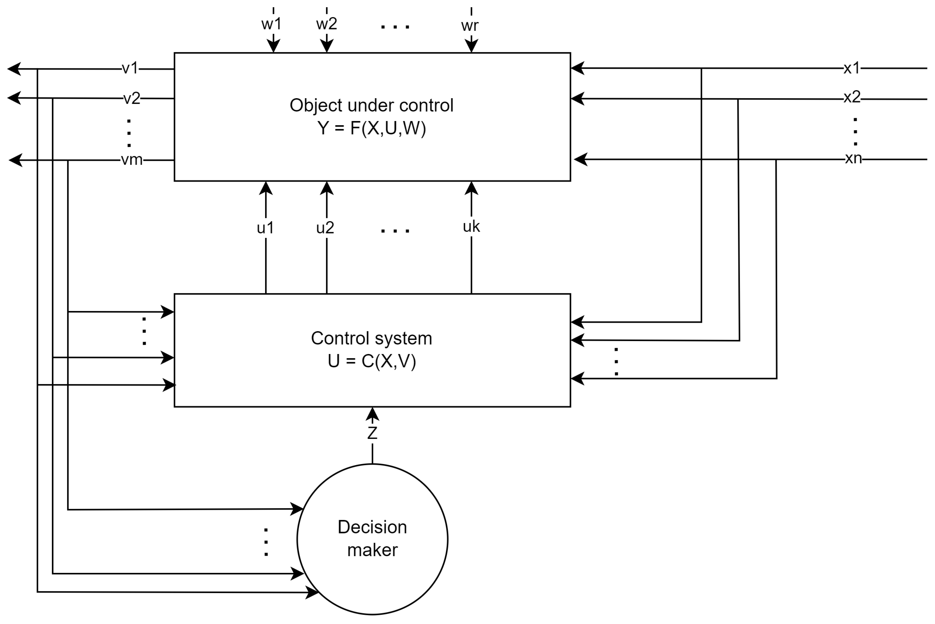
  • The input of the control object is the vector X = { x 1 , , x n } .
  • The control object is also regulated by the vector W = { w 1 , , w r } . The values of the vector W cannot be determined.
  • The output of the control object is the vector V = { v 1 , , v n } .
  • The feedback vector from the control system U = { u 1 , , u k } also comes to the input of the control object.
There are various approaches to control complex technical systems that provide control stability. For example, deterministic models as mathematical dependencies can be used for this task. Intelligent components and components based on machine learning can be used for systems with non-linearity and/or uncertainty in the behavior of a control object [2]. The use of forecasting methods allows us to reduce the response time of the system to emerging deviations. Predictive models have the disadvantage of needing to choose the appropriate volume of data to build a forecast and evaluate the quality of this data.
Neural networks can be a solution for a control task. A neural network is a black box model that can accurately estimate complex non-linear relationships. Fuzzy modeling also can be used for solving the control task. Fuzzy modeling is a modeling method that uses a fuzzy inference system based on fuzzy rules [3]. Hybrid solutions that overcome the limitations of existing individual models allow us to obtain new results from both. One such model is ANFIS. However, the development of methods and algorithms based on artificial intelligence requires several experiments to produce the required configuration and accuracy of the models. In addition, if the data contain incompleteness, noise, or gaps, the results of the work of intelligent models will be of poor quality [4,5].
There are several control systems types. The first class includes automatic control systems. The role of the decision maker is minimized in these systems [6,7]. Automatic control systems are often based on PID controllers with various types of models. Another class of systems is the decision support system. This class of systems is actively used by decision makers in various management tasks. A hierarchical approach to the decomposition of data analysis and decision-making tasks is possible in decision support systems [8].
The directions for the development of intellectual methods are [9]:
  • The expansion of the set of analyzed data;
  • The complication of the applied models;
  • The increase in the interpretability of the results;
  • The explainability of the result.
Authors in the article [10] noted that the use of additional information can improve the quality of modeling.
Researchers often use time series models to identify the patterns of changes in indicators. Time series models are based on methods of trend analysis and various methods for correlations. Correlation methods allow us to identify relationships between indicators of a single object or between indicators of different objects. These methods are based on an analysis of object attributes in dynamics. Statistical, fuzzy, and neural network models of time series allow solving these tasks, depending on the type of data [11].

3. The Problem Statement

In our study, we use a hybrid approach. The novelty of the proposed approach is the use of contextual information about the analysed object, such as dependencies, restrictions, and relationships. We use a priori information specified in the context of objects of the organizational and technical system instead of searching for dependencies through the analysis of time series.
It is necessary to change the scheme of the common control process (Figure 1) to apply the proposed approach. The new block allows for modeling dynamic parameters and using context data. The new block is not part of the control system because it provides information to the decision maker and/or to the automatic control system. This solution is not a decision support system in the classic sense, but it allows increased flexibility of the control process. We plan to continue improving the contextual analysis of the dynamics of object attributes in the future. We also plan to apply the approach to unmanned vehicles in agriculture for automatic planning and tracking the movement trajectory. The modified scheme is shown in Figure 2.
Let us consider the new block in more detail. The contextual and dynamic decision support block has the following properties:
  • Input to obtain external information about the control context D of a control object;
  • Input to accumulate the dynamics of a control object attributes (vector V);
  • Management recommendations R e s as the output (recommendations for decision maker and/or numerical values to regulate the behavior of a control object).
Software development based on agile methodologies is the example of a problem area used for the proposed approach demonstration. Timely response to emerging events is especially important in this domain because it allows implementing aspects such as inspection and adaptation in conditions of extreme development parameters [12].
The indicators of quality in a model software system include functionality (measured by the number of implemented tasks with new functionality), performance (measured by the time it takes to execute functions), and reliability (measured by the number of unhandled exceptions) [13].
The indicators of a quality model during the development process include mainly internal project quality indicators: efficiency (measured by the test execution time, project build time, the ratio of the number of implemented functionality to the number of developers), reliability (measured by the number of errors during static testing of the code, test coverage), and fulfillment of requirements (measured by the duration of the development tasks).
Note that this selection of parameters does not pretend to be original. These parameters are just used to demonstrate the proposed approach in the project management task. The main aim is to reduce the time required for obtaining information about the critical levels of quality models.

4. Control Models

Let us present the necessary models for the block of contextual analysis of the dynamics of indicators of the proposed scheme as shown in Figure 2. A significant difference from the traditional control scheme is the availability of information about related objects.
Building a model for managing a complex technical system must begin with the selection of a set of analyzed objects and their properties.
Let O = { o 1 , o 2 , , o n } be a set of such objects, where n N . For each object, we define a set of attributes that characterizes the state of the object: o j = { v i o j } , where v i o j is the numerical value of the indicator i for the analyzed object o j . In the scheme in Figure 2, such a set of attributes for a control object are represented by the vector V = { v 1 , , v m } . These indicators are the basis for the time series of indicators. They help implement the principle of dynamics of indicators, see (1)
T S ( v i o j , t ) t s i o j ,
where T S is the function that creates the time series of the indicator i of the object o j , t is the time of the fixation the value of the indicator, and t s i o j is the time series of the indicator i object o j .
The relations between the objects of the problem area must be considered in order to analyze the mutual influence of their states and track dependencies.
Take the case of R k l = r o k o l , where r o k o l characterizes the object connection degree between o k and object o l . The relation degree is a numerical characteristic involved in the analysis of the dynamics of indicators. It shows how the selected indicator positively or negatively affects the state of the associated object. When solving the control problem, such a relation helps to achieve the principle of decomposition. The limited set of related objects makes it possible to determine the criteria for achieving a stable state of the control system based on the proposed models. Instead of the relationship degree of one object to another, we can use the object attributes relationship degree for more flexibility.
Calculating the dependency degree of the attributes of one object on the parameters of another is expressed as a function, see (2).
f ( R k l ) = t s t + 1 o k r o k o l
Such functionality allows us to calculate the state or adjust the control process in the following scenarios:
  • The state and reliable trends of changes in the values of attributes of one object are known. It is possible to predict the value of the attribute associated with the source object by the presented functional dependence: v i o j = v i o k r o k o l , where v i o j is the predicted value of i-th attribute j-th object, or in the form of a time series forecast: t s t + 1 o j = t s t + 1 o k r o k o l
  • We do not know the trends in the values of related objects, but there are predictive values. Using these values, it is possible to diagnose the values of the attributes | v i o j v i o k | .
Control actions on the control object are defined by the control task after analyzing the deviations of the output indicators of the control object from the reference ones, see (3).
| v i o j e o j | 0 , i , j ,
where v i o j is the value of the i-th attribute of the j-th object, and e i o j is the reference value.
An exact match of the values is not achieved, and it is required to set some intervals boundaries of acceptable values. We can express a vector for each object, see Equation (4).
Δ o j = { δ i o j } | v i o j e o j | δ i o j , i , j .
To implement the principle of adaptability, we specify intervals of acceptable values as fuzzy labels Δ ˜ o j .
As a result, we denote the function implemented by the control model of the function (5).
D = < O , Δ ˜ O , R > , C o n t r o l ( D , T S M o d e l s ) R e s ,
where D is an ontology that describes the links of the objects of analysis O by setting the weight of the link R and includes restrictions on the values of the attributes of the control object Δ ˜ O based on the ontology and a set of models, time series T S M o d e l s , recommended for managing R e s as consequential rules for responding to deviations.

5. Analysis Algorithm

According to the scheme shown in the Figure 2, it is necessary to determine the order of operation of the block for contextual analysis of the dynamics of indicators. The algorithm given below concerns only the operation of this block and is not a description of the entire control task. The complex of models in solving the control problem is a set of prognostic models of time series T S M o d e l s , a knowledge base model for the context of modeling time series D, and a control model based on fuzzy logical inference during the operation of the system of rules C o n t r o l ( D , T S M o d e l s ) R e s .
Let us describe the algorithm used for the decision-making procedure in solving control problems.
  • Form an ontology D that describes the relationships between objects and attributes.
  • Generate time series of values of indicators of the studied objects v i o j . Instead of a single output vector of the control object, it is necessary to present the history of each indicator T S ( v i o j , t ) t s i o j .
  • Describe the context in the ontology D as rules for performing fuzzy inference when working with predictive T S M o d e l s , their parameters, and types.
  • Select and train fuzzy predictive T S M o d e l s to adapt to the features of the selected objects. The results are presented in more detail in [14].
  • Make a forecast based on incoming data and context.
  • Evaluate the result on test data | v i o j e o j | .
  • If the quality is satisfactory, make a forecast for the next management period and adjust the management parameters R e s based on the forecasts; otherwise, choose other predictive models.
The comparison procedure with reference values during testing works on fuzzy values and rules defined in the ontology. This is not able to set the exact values of the error thresholds, but it can be used as fuzzy labels Δ ˜ o j .

6. Quality Assessment

Evaluation of the quality of the models is a multi-level process. There are some metrics that include a metric for assessing the quality of time series modeling and a metric for assessing the quality of a management model.

6.1. Time Series Quality Assessment

One of the metrics for assessing the quality of time series forecasting is the SMAPE [15] criterion. The expression (6) represents the calculations of the metric
S M A P E = 100 % n t = 1 n | F t A t | ( | A t | + | F t | ) / 2 .
where F t is t-th forecasted value, A t is t-th real value, and n is the forecast horizon.
The value of the forecast error by the SMAPE criterion affects the choice of the time series model when the algorithm is running.

6.2. Total Quality Assessment

The quality coefficient (the lower the better) of the management model is to measure the discrepancy between the output of the model and the referenced value. Let us express this as functional (7).
Q t o t a l = i , j | v i o j e i o j | δ i o j m i n ,
where v i o j is the predicted value of the i-th attribute of the j-th object when testing the model, e i o j is the reference value when testing the model, and δ i o j is the maximum deviation from the reference value of the i-th attribute of the j-th object.
The error rate and the difference | v i o j e i o j | are used to make recommendations for management.

7. Ontology for Representing the Context of a Control Problem

The solution to the control problem involves considering the features of both the control object itself and the domain [16,17]. In addition, the control object functions under the limitations of the restrictions of some domain. We define these features and limitations as the context of the control problem (context).
We use ontologies to describe the context of a control problem.

7.1. Description Logic

Ontologies are an effective instrument of describing the context for solving various automation problems [18]. Ontologies combine tools for describing the features of a domain, components for the formation and execution of a set of production rules, and a set of inference engines. The process of inference forms new knowledge based on ontology constraints and/or a set of production rules in the SWRL language [19]. In addition, the inference engine controls the consistency of ontology axioms.
Ontologies are based on various description logic languages. Description logic makes it possible to guarantee the decidability of ontology axioms at low computational costs. Currently, the OWL 2 standard is used to represent ontologies [20,21,22].
Table 1 contains description logic operators and axioms for representing the elements of the proposed ontology.

7.2. Model of the Proposed Ontology

We propose an OWL 2 ontology of the following structure to describe the context of a control problem:
D = O D , F D , E D , R D ,
where
O D is an ontological representation of objects of analysis O;
F D is an ontological representation of a set of modeling methods of time series;
E D is an ontological representation of expert knowledge to implement management functions;
R D is a set of relationships between ontology components.
We present the ontology D of the context of the control problem using a dialect of ALCHONF ( D ) description logic:
D = D T B o x , O T B o x D , O A B o x D , F T B o x D , F A B o x D , E T B o x D , E A B o x D ,
where
T B o x is a set of terminological axioms;
A B o x is a set of axioms.

7.3. Terminology of the Proposed Ontology ( T B o x )

The common terminology of the D ontology is:
h a s N a m e . S t r i n g h a s N a m e . S t r i n g = 1 h a s N a m e . S t r i n g ,
where h a s N a m e is a functional role common to all ontology classes.
The terminology for representing analysis objects ( O T B o x D ) can be described as the following axioms:
  • The terminology O T B o x D contains a set of classes for describing:
    Analyzed objects— O b j e c t ;
    Properties (attributes) of an object— A t t r i b u t e ;
    The time series of values of an object attribute— T S ;
    Dependencies between attributes of objects— D e p e n d e n c y ;
    Types of dependencies: positive, negative— D e p e n d e n c y T y p e :
    O b j e c t A t t r i b u t e T S D e p e n d e n c y D e p e n d e n c y T y p e { p o s i t i v e , n e g a t i v e } ;
  • The classes O b j e c t , A t t r i b u t e , T S , D e p e n d e n c y , and D e p e n d e n c y T y p e are declared as disjoint:
    O b j e c t A t t r i b u t e T S D e p e n d e n c y D e p e n d e n c y T y p e ;
  • The O b j e c t class has the h a s A t t r i b u t e role to specify a tie between some object and a set of its attributes:
    O b j e c t h a s A t t r i b u t e . A t t r i b u t e ;
  • The A t t r i b u t e class has:
    Functional roles h a s D e l t a M i n and h a s D e l t a M a x to define the minimum and maximum value of an attribute;
    The h a s D e p e n d e n c y role to specify a tie between attributes of analyzed objects;
    The functional role h a s T S to define a tie between an attribute and time series that contains a dynamic of an attribute:
    A t t r i b u t e h a s D e l t a M i n . D o u b l e = 1 h a s D e l t a M i n . D o u b l e h a s D e l t a M a x . D o u b l e = 1 h a s D e l t a M a x . D o u b l e h a s D e p e n d e n c y . D e p e n d e n c y h a s T S . T S h a s T S . T S = 1 h a s T S . T S ;
  • The T S class has the h a s D a t a functional role to define a source of time series data:
    T S h a s D a t a . S t r i n g h a s D a t a . S t r i n g = 1 h a s D a t a . S t r i n g ;
  • The D e p e n d e n c y class has:
    The functional role d e p e n d s O n to organize dependencies between object attributes;
    The functional role h a s T y p e to define the dependency between attributes;
    The functional role h a s W e i g h t to determine a weight of dependency between attributes:
    D e p e n d e n c y d e p e n d s O n . A t t r i b u t e d e p e n d s O n . A t t r i b u t e = 1 d e p e n d s O n . A t t r i b u t e h a s T y p e . D e p e n d e n c y T y p e h a s T y p e . D e p e n d e n c y T y p e = 1 h a s T y p e . D e p e n d e n c y T y p e h a s W e i g h t . D o u b l e h a s W e i g h t . D o u b l e = 1 h a s W e i g h t . D o u b l e .
The terminology of representation of modeling methods of time series ( F T B o x D ) contains the following axioms:
  • The terminology F T B o x D contains a set of classes for describing:
    Methods for time series modeling— M e t h o d ;
    The features of time series that a method supports: fuzziness, periodicity, smoothing, trends— M e t h o d F e a t u r e :
    M e t h o d M e t h o d F e a t u r e { f u z z y , p e r i o d i c , s m o o t h , t e n d e n c y } ;
  • The classes M e t h o d and M e t h o d F e a t u r e are declared as disjoint:
    M e t h o d M e t h o d F e a t u r e ;
  • The M e t h o d class has:
    The h a s F e a t u r e role to define a tie between the method and its features;
    Functional roles h a s L e n g t h M i n and h a s L e n g t h M a x to determine the minimum and maximum lengths of time series that the method supports:
    M e t h o d h a s F e a t u r e . M e t h o d F e a t u r e h a s F e a t u r e . M e t h o d F e a t u r e > = 1 h a s F e a t u r e . M e t h o d F e a t u r e h a s L e n g t h M i n . I n t e g e r = 1 h a s L e n g t h M i n . I n t e g e r h a s L e n g t h M a x . I n t e g e r = 1 h a s L e n g t h M a x . I n t e g e r ;
  • In addition, the additional n e e d F e a t u r e role is defined for the T S class in the terminology O T B o x D . The n e e d F e a t u r e role allows declaring a tie between time series and its features:
    T S n e e d F e a t u r e . M e t h o d F e a t u r e n e e d F e a t u r e . M e t h o d F e a t u r e > = 1 n e e d F e a t u r e . M e t h o d F e a t u r e .
The terminology for representing expert knowledge ( E T B o x D ) can be described as the following axioms:
  • The terminology E T B o x D contains a set of classes for describing:
    Expert knowledge— E x p e r t ;
    A value of some attribute of the object at a certain point of a time series— P o i n t ;
    States in which an object is located— S t a t e . A set of states of an object is based on a value of some object attributes. The S t a t e class extends the E x p e r t class;
    Actions to correct a value of some object attribute— R e s u l t . The R e s u l t class extends the E x p e r t class:
    E x p e r t P o i n t S t a t e E x p e r t R e s u l t E x p e r t ;
  • The classes S t a t e , R e s u l t , and P o i n t are declared as disjoint:
    S t a t e R e s u l t P o i n t ;
  • The E x p e r t class has the functional role h a s D e s c r i p t i o n common to all classes of expert knowledge:
    E x p e r t h a s D e s c r i p t i o n . S t r i n g h a s D e s c r i p t i o n . S t r i n g = 1 h a s D e s c r i p t i o n . S t r i n g ;
  • The P o i n t class has:
    The functional role h a s I n d e x to associate a value of some attribute with a specific point of a time series,;
    The functional role h a s R e s u l t to define actions to correct a value of some object attribute;
    The functional role h a s V a l u e to define a value of an attribute at some point in a time series;
    The functional role f o r A t t r i b u t e to associate some point of a time series with an object attribute:
    P o i n t h a s I n d e x . I n t e g e r h a s I n d e x . I n t e g e r = 1 h a s I n d e x . I n t e g e r h a s S t a t e . S t a t e h a s S t a t e . S t a t e = 1 h a s S t a t e . S t a t e h a s R e s u l t . R e s u l t h a s R e s u l t . R e s u l t = 1 h a s R e s u l t . R e s u l t h a s V a l u e . D o u b l e h a s V a l u e . D o u b l e = 1 h a s V a l u e . D o u b l e f o r A t t r i b u t e . A t t r i b u t e f o r A t t r i b u t e . A t t r i b u t e = 1 f o r A t t r i b u t e . A t t r i b u t e .

7.4. Axioms of the Proposed Ontology ( A B o x )

A set of facts A B o x of the proposed ontology is formed automatically using special screen forms to automate the work of an expert.
The following steps are used to form the axioms ( O T B o x D ) for the control problem:
  • Specification of objects:
    o b j e c t 1 : O b j e c t ( o b j e c t 1 , S o m e o b j e c t ) : h a s N a m e .
  • Specification of the attributes for each object. Each attribute specifies a data source and a valid range of values:
    t s 1 : T S ( t s 1 , S o m e t i m e s e r i e s ) : h a s N a m e ( t s 1 , . . / d a t a / t s 1 . c s v ) : h a s D a t a a t t r i b u t e 1 : A t t r i b u t e ( a t t r i b u t e 1 , S o m e a t t r i b u t e ) : h a s N a m e ( a t t r i b u t e 1 , 0.5 ) : h a s D e l t a M i n ( a t t r i b u t e 1 , 11.6 ) : h a s D e l t a M a x ( a t t r i b u t e 1 , t s 1 ) : h a s T S ( o b j e c t 1 , a t t r i b u t e 1 ) : h a s A t t r i b u t e .
    Currently, only one-dimensional time series in CSV format are supported.
  • Specification of dependencies between object attributes:
    d e p e n d e n c y 1 : D e p e n d e n c y ( d e p e n d e n c y 1 , a t t r i b u t e 2 ) : d e p e n d s O n ( d e p e n d e n c y 1 , p o s i t i v e ) : h a s T y p e ( d e p e n d e n c y 1 , 0.85 ) : h a s W e i g h t ( a t t r i b u t e 1 , d e p e n d e n c y 1 ) : h a s D e p e n d e n c y .
The following query in the SQWRL language is used to obtain a list of dependencies for the selected attribute of some object:
h a s D e p e n d e n c y ( a t t r i b u t e 1 , ? d ) h a s T y p e ( ? d , p o s i t i v e ) d e p e n d s O n ( ? d , ? a d e p ) h a s W e i g h t ( ? d , ? w ) s q w r l : s e l e c t ( a t t r i b u t e 1 , ? a d e p , ? w )
It is also necessary to add to the ontology the information about the modeling methods of time series and specify their features:
m e t h o d 1 : M e t h o d ( m e t h o d 1 , F t r a n s f o r m ) : h a s N a m e ( m e t h o d 1 , s m o o t h ) : h a s F e a t u r e ( m e t h o d 1 , f u z z y ) : h a s F e a t u r e ( m e t h o d 1 , p e r i o d i c ) : h a s F e a t u r e ( t s 1 , p e r i o d i c ) : n e e d F e a t u r e ( t s 1 , f u z z y ) : n e e d F e a t u r e .
The following SQWRL query can be used to obtain suitable time series modeling methods:
M e t h o d ( ? m ) h a s F e a t u r e ( ? m , ? m f ) s q w r l : m a k e S e t ( ? m f s e t , ? m f ) s q w r l : g r o u p B y ( ? m f s e t , ? m ) h a s T S ( a t t r 1 , ? t s ) n e e d F e a t u r e ( ? t s , ? a f ) s q w r l : m a k e S e t ( ? a f s e t , ? a f ) s q w r l : c o n t a i n s ( ? m f s e t , ? a f s e t ) s q w r l : s e l e c t ( ? m ) .
An expert needs to execute the following steps to form axioms of expert knowledge representation ( E T B o x D ):
  • Specification of a set of states for some attribute and a membership function to make fuzzification of attribute values [23]:
    l o w : S t a t e ( l o w , L o w s t a t e ) : h a s D e s c r i p t i o n m i d d l e : S t a t e ( m i d d l e , M i d d l e s t a t e ) : h a s D e s c r i p t i o n h i g h : S t a t e ( h i g h , H i g h s t a t e ) : h a s D e s c r i p t i o n .
    A more detailed description of the fuzzy inference module is presented in the Section 7.5.
  • Specification of a set of actions to correct a value of some object attribute:
    r e s u l t 1 : R e s u l t ( r e s u l t 1 , S o m e r e s u l t ) : h a s D e s c r i p t i o n r e s u l t 2 : R e s u l t ( r e s u l t 2 , A n o t h e r r e s u l t ) : h a s D e s c r i p t i o n .
  • Specification of a set of SWRL-rules for transition from states to results:
    f o r A t t r i b u t e ( ? p 1 , a t t r 1 ) h a s S t a t e ( ? p 1 , l o w ) f o r A t t r i b u t e ( ? p 2 , a t t r 2 ) h a s S t a t e ( ? p 2 , m i d d l e ) f o r A t t r i b u t e ( ? p 3 , a t t r 3 ) h a s S t a t e ( ? p 3 , l o w ) h a s R e s u l t ( p 1 , r e s u l t 1 ) f o r A t t r i b u t e ( ? p 1 , a t t r 1 ) h a s S t a t e ( ? p 1 , m i d d l e ) f o r A t t r i b u t e ( ? p 2 , a t t r 2 ) h a s S t a t e ( ? p 2 , m i d d l e ) f o r A t t r i b u t e ( ? p 3 , a t t r 3 ) h a s S t a t e ( ? p 3 , l o w ) h a s R e s u l t ( p 1 , r e s u l t 2 ) .
    The rules are based on the states of the attributes at a certain point in time (a point in a time series) through the ‘forAttribute’ role.

7.5. Fuzzy Inference

Conclusions about the state of some objects based on the analysis of their attribute values are formed with fuzzy inference. The following concepts of the fuzzy sets theory are used for fuzzy inference [24,25]:
  • Membership functions;
  • Linguistic variables;
  • Fuzzy implication methods.
A membership function in fuzzy logic determines a membership degree of the elements of a universal set to some fuzzy set.
The fuzzy set for a universal set U and a membership function μ : U [ 0 , 1 ] is defined as [24,25]:
A ˜ = { u , μ A ( x ) | u U } .
Membership function μ A ( x ) quantitatively grades the membership of the elements of a universal set u U to a fuzzy set A ˜ . Membership degree zero means that an element is not included in a fuzzy set, and membership degree one describes a fully included element. Values between zero and one represent fuzzy included elements.
A linguistic variable in the fuzzy set theory takes the semantic of terms in a natural or formal language. Terms represent fuzzy variables and are described by a fuzzy set.
A linguistic variable can be represented as an expression [25]:
L T = { x , T ( x ) , X , G , M } ,
where x is a variable name, and T ( x ) is a set of values of a linguistic variable x. Each value of a set is a fuzzy variable on a set X; G is a is a set of additional features for generating new x values; M is a mathematical rule for determining the type of membership function for each value formed based on a G set.
For example, for the linguistic variable ‘employees number’ (Figure 3):
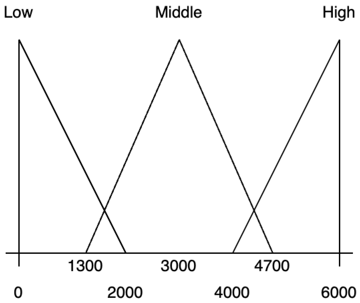
  • x is an employees number;
  • X a set of integers from the range [0, 6000];
  • T ( x ) is a set of fuzzy variables: ‘low’, ‘middle’, ‘high’. It is necessary to set a membership function that specifies information about what employees number should be considered ‘low’, ‘middle’, or ‘high’;
  • G is a set of additional features: ‘less than’, ‘more than’. Additional features are used to create new fuzzy variables. For example, ‘less than middle’ and ‘more than low’, etc.
Fuzzy inference is executed based on fuzzy rules. A set of fuzzy rules form a fuzzy production system in the context of some subject area. A fuzzy rule can be represented as the expression:
R = K , E , W ,
where K is the core of a fuzzy rule of the following form:
K = A C ,
where A = { A 1 , A 2 , , A i , , A n } is an antecedent of a rule consisting of many atoms A i ; and C = { C 1 , C 2 , , C i , , C k } is a consequent of a rule consisting of atoms C i . Atoms of a fuzzy rule must represent single and compound statements connected by binary operations AND and OR. In SWRL-rules, the ∧ operator represents the AND operation, and multiple queries represent the OR operation; the E function determines a truth degree (from range (0; 1)) of a fuzzy rule result; W is a fuzzy rule weight. If rule weight is not defined, then the weight is one.
The fuzzy inference module uses the Mamdani algorithm. The fuzzy inference consists of the following steps:
  • Fuzzification. Fuzzification is used to switch from numerical indicators of object properties to linguistic variables. The values of all input variables are associated with specific values of the membership functions of linguistic terms from antecedents of fuzzy rules at the fuzzification stage.
    A set of attribute states is formed in the process of fuzzy inference based on the values of time series points (‘hasValue’ role). Each point of a time series is associated through the ‘hasState’ role with a corresponding linguistic term in the process of fuzzy inference [23]. The ‘hasState’ role describes a membership of some time series point to a certain fuzzy set with some degree of membership:
    p o i n t i : P o i n t ( p o i n t i , i ) : h a s I n d e x ( p o i n t i , s j S t a t e ) : h a s S t a t e .
  • Aggregation. A truth degree of antecedents for each rule is determined at the aggregation stage. If an antecedent of a fuzzy rule contains one atom, then a truth degree of an antecedent is a truth degree of this atom. A truth degree of an atom is calculated based on the value of a membership function of a linguistic variable term. If an antecedent of a rule contains several atoms, then a truth degree is calculated based on the truth degrees of the antecedent atoms using fuzzy logic AND ( m i n ) operator.
  • Activation. A truth degree of each consequent atom of the fuzzy rule is determined at the stage of activation. A truth degree of each consequent atom is equal to the algebraic product of a rule weight and a truth degree of a rule antecedent. If weights of production rules are not specified, then their default values are equal to one. Minimum is used to calculate truth degrees.
    A Set of results for object control is formed as a result of the inference. It is possible to obtain results for each point of a time series or for the individual points. Fuzzy inference allows obtaining a set of solutions ordered by their degree of truth. The degree of truth is calculated at the stages of aggregation and activation of the fuzzy inference [23]. For example:
    AttributeResultResult descriptionTruth degree
    attr1result1Some result0.356
    attr1result2Another result0.047
  • Accumulation. A membership function is formed for each linguistic variable from the consequent fuzzy rules at the accumulation stage. Accumulation is based on the union of fuzzy sets of all consequent atoms for some linguistic variable using fuzzy logic OR ( m a x ) operator.
  • Defuzzification. The result of defuzzification is quantitative (crisp) values for each output linguistic variable based on the results of the accumulation of all output linguistic terms from the consequences of fuzzy rules using the center of gravity method.
As you can see from Figure 2, the proposed fuzzy inference mechanism can produce two types of results:
  • A set of recommendations for decision makers ordered by truth degree. The result is formed at the aggregation step, the accumulation and defuzzification steps are not required.
  • A set of numerical values to regulate the behavior of the object. All steps must be completed.
Thus, the proposed ontology model makes it possible to form a context for solving the control problem. Creation of axioms for the proposed ontology does not require knowledge of special tools from an expert. Using fuzzy inference makes it easier to form a set of SWRL-rules.

8. Results

We will consider the analysis according to the scheme in Figure 2. The object under control is the software project development process. The vector of input parameters X = { x 1 , , x n } will be a set of requirements for developers: a list of tasks to be implemented and time limits. The output data V = { v 1 , , v m } of the control object will be artifacts and indicators extracted from the git repositories of the program code, testing systems, and source code analysis.
By themselves, the values of these parameters may not reflect the actual state of the project being implemented. Therefore, we introduce an integrated assessment, which makes it possible to track the influence of input data, control actions and random influences as a quality assessment in dynamics.
Two main sections: product quality and quality of development processes, represent software development quality models. Development management keeps track of both key metrics. Therefore, it is possible to identify development indicators that will influence the formation of quality. For each indicator, the history of the value change as a time series is retrieved.
We show the application of the proposed approach on one of the software projects to automate the activities of the university research group [26]. Junior programmers developed the project over several months.
The source data for analysis are the indicators of the git source code repository, which reflects the indicators of the development process and its results. We host the repository on the GitLab service, which allows storing and versioning the source code, to automate development processes: building and testing the project, keeping statistics, and managing project tasks.
Let s provide a description of each indicator. The indicator values are average values over a weekly time interval.
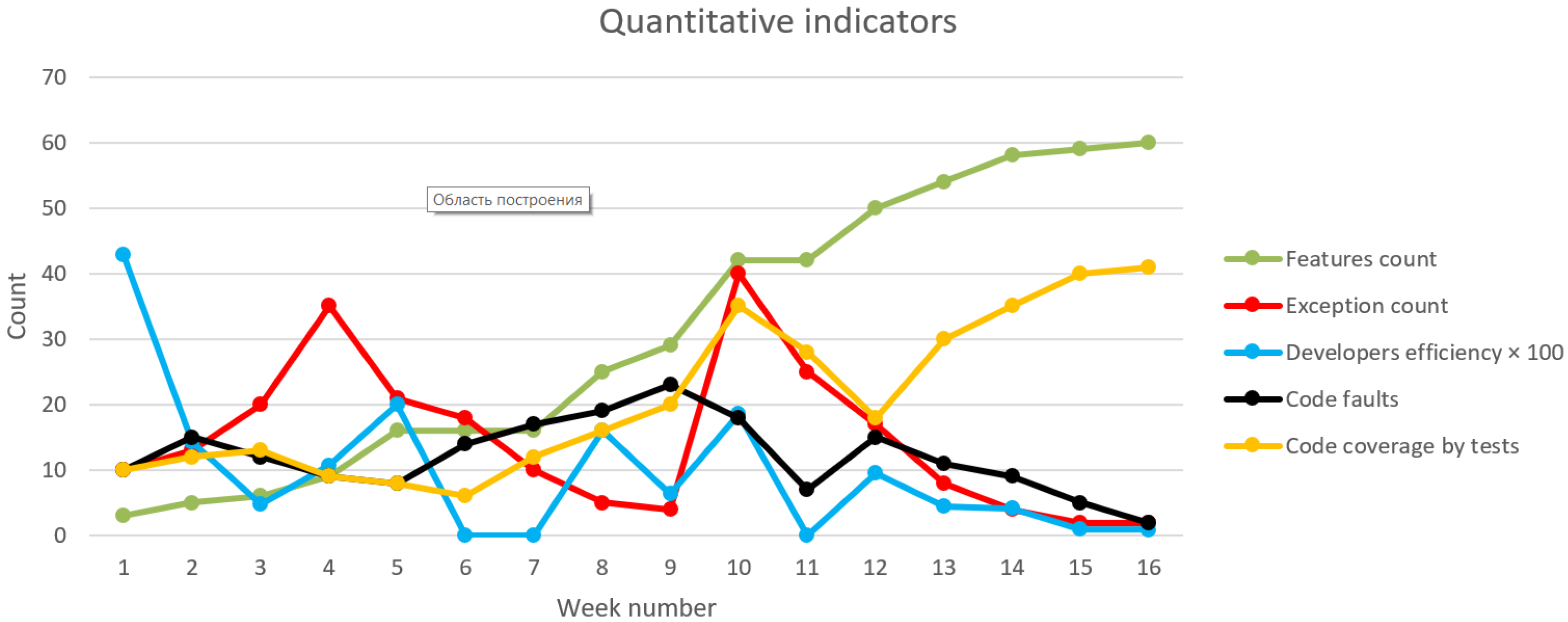
  • The number of features is determined by the number of issues (issue) in the “Implemented” state.
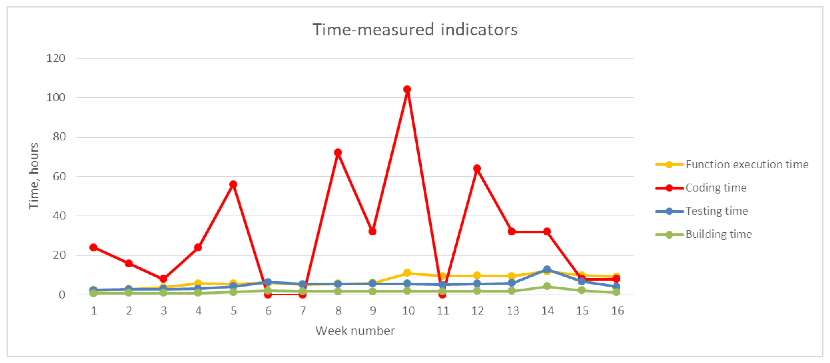
  • Feature execution time is determined by the cumulative execution time of automated tests.
  • Exception count is the sum of all exceptions found during testing.
  • Test time is the cumulative runtime of unit tests.
  • Project build time is the average time of compilation of a project and running in automatic mode to check if it works.
  • Efficiency of developers is determined by the number of completed tasks in a weekly interval.
  • Bugs in the code are determined using the SonarQube service to obtain an indicator of the static code analysis system.
  • Code test coverage shows the measure of checking all the implemented functionality with unit tests.
  • Code writing time reflects a measure similar to developer efficiency, the time developers spend on tasks. However, unlike the first indicator, the measurement of this indicator does not include such overhead costs as task management, life cycle changes, discussion, and testing costs.
Table 2 also lists the weights of indicator links that affect quality models. That is, for example, the relationship between the problem area object “Product Quality” and “Number of Features” is ranked by weight five.
By the steps of the algorithm (see the Section 5), the ontology describes choosing methods for predicting time series and relationships between analyzed objects (see the Section 7.2).
Figure 4 and Figure 5 show examples of extracted time series.
Forecast values of indicators allow making a logical inference in the ontology. These forecasted values are input as parameters according to the trends in the time series of indicators, as shown in Table 3. In this experiment, the forecast horizon was based on known real values to help assess the quality of the forecasts. The test forecast horizon covers time series points from 11 to 16. The described earlier in [27] approach forecasts by choosing a model suitable for the time series context.
Forecast values represent only a single trend value per forecast interval (for simplicity). Based on the forecast data and information from the ontology about the allowable change intervals, the following indicators have deviations: exception count, building time, and testing time parameters. The values of these indicators are inflated compared to the model’s predicted values.
Previously, there were certain links between indicators and objects of management—the quality of development processes and the quality of a software product. This relationship can explain why the state of the control object is deteriorating and in what proportion.
In the compiled ontology, the boundaries of the permissible values of indicators, as well as the rules for responding to exceeding the boundaries, are determined.
Let us assess the control object indicators based on the forecast values as shown in Table 4. We made the calculation considering the normalized values because the weights of the r o k o l indicators according to (2) are already normalized relative to each other, and the absolute values of the indicators can differ greatly. We normalize considering the maximum value among the current and forecast values of indicators. For example, for the “Features count” indicator, the maximum value will be 63. Further, using the formula v a l u e w e i g h t , we will recalculate the values of indicators from the Table 3.
The values from Table 4 are used to calculate the integral quality index Q t o t a l . The value of the software system quality model reflects a higher value of the quality of the software product. It was the primary target of the development of the software project, and the indicators of the quality model of the development processes significantly worsened its total value. Predictive models reflected this state. The final assessment of the quality is Q t o t a l = 5.94.
During the implementation of the project, we made organizational changes. We changed the test environment (continuous integration server) and the logic for testing developers’ code changed. These changes allowed us to improve the indicators “|Testing time” and “Project build time”. After the changes, Q t o t a l was 2.75.

9. Conclusions

The results presented in this article develop a previously proposed approach for the contextual analysis of indicators of objects in the problem area, expressed as time series. This approach helps obtain a set of models that reflect the features of the analyzed objects, reduces the burden on experts, and has complete possibilities for interpreting the simulation result.
This article showed an approach to solving a control problem based on the dynamics of changes in the indicators of a set of objects in the problem area.
The advantages of this approach are the ability to use more complete data for making management decisions, as well as reducing the analysis time through the use of intelligent models. Thus, the experiment conducted on the data of the git repository of the program code showed that the proposed approach also made it possible to increase the explainability of the analysis results. We show the difference between the proposed approach as a hybrid solution between traditional control systems and a decision support system.
Further work within the framework of this study involves the creation of a control system for solving problems of automatic control based on the analysis of the context of the dynamics of changes in the parameters of objects.

Author Contributions

Conceptualization, A.A.R.; data curation, A.A.F.; formal analysis, A.A.F.; methodology, N.G.Y.; visualization, A.A.R. All authors contributed equally. All authors have read and agreed to the published version of the manuscript.

Funding

This research was funded by the Ministry of Science and Higher Education of the Russian Federation in the framework of the state task No. 075-00233-20-05 “Research of intelligent predictive multimodal analysis of big data, and the extraction of knowledge from different sources”.

Institutional Review Board Statement

Not applicable.

Informed Consent Statement

Not applicable.

Data Availability Statement

Not applicable.

Conflicts of Interest

The authors declare no conflict of interest.

References

  1. Pospelov, D.A. Situational Management: Theory and Practice; Fizmatlit: Moscow, Russia, 1986. (In Russian) [Google Scholar]
  2. Xu, J.; Wang, Q.; Lin, Q. Parallel robot with fuzzy neural network sliding mode control. Adv. Mech. Eng. 2018, 10, 1687814018801261. [Google Scholar] [CrossRef]
  3. Nguyen, A.-T.; Taniguchi, T.; Eciolaza, L.; Campos, V.; Palhares, R.; Sugeno, M. Fuzzy Control Systems: Past, Present and Future. IEEE Comput. Intell. Mag. 2019, 14, 56–68. [Google Scholar] [CrossRef]
  4. Tabbussum, R.; Dar, A.Q. Performance evaluation of artificial intelligence paradigms—Artificial neural networks, fuzzy logic, and adaptive neuro-fuzzy inference system for flood prediction. Environ. Sci. Pollut. Res. 2021, 28, 25265–25282. [Google Scholar] [CrossRef]
  5. Frazzon, E.M.; Kück, M.; Freitag, M. Data-driven production control for complex and dynamic manufacturing systems. CIRP Ann. 2018, 67, 515–518. [Google Scholar]
  6. Bejarano, G.; Alfaya, J.A.; Rodríguez, D.; Morilla, F.; Ortega, M.G. Benchmark for PID control of refrigeration system based on vapour compression. IFAC PapersOnLine 2018, 51, 497–502. [Google Scholar]
  7. Márquez-Vera, M.A.; Ramos-Fernández, J.C.; Cerecero-Natale, L.F.; Lafont, F.; Balmat, J.F.; Esparza-Villanueva, J.I. Temperature control in a MISO greenhouse by inverting its fuzzy model. Comput. Electron. Agric. 2016, 124, 168–174. [Google Scholar] [CrossRef]
  8. Kotenko, I.; Saenko, I.; Ageev, S. Hierarchical fuzzy situational networks for online decision-making: Application to telecommunication systems. Knowl.-Based Syst. 2019, 185, 104935. [Google Scholar] [CrossRef]
  9. Petrushevskaya, A.A. Control model of technological operations of mounting automatic printed circuit boards based on a multiparameter fuzzy classifier. J. Phys. Conf. Ser. 2019, 1333, 042026. [Google Scholar]
  10. Morales Escobar, L.; Aguilar, J.; Garcés-Jiménez, A.; Gutierrez De Mesa, J.A.; Gomez-Pulido, J.M. Advanced Fuzzy-Logic-Based Context-Driven Control for HVAC Management Systems in Buildings. IEEE Access 2020, 8, 16111–16126. [Google Scholar] [CrossRef]
  11. Novák, V.; Mirshahi, S. On the Similarity and Dependence of Time Series. Mathematics 2021, 9, 550. [Google Scholar] [CrossRef]
  12. What Is Scrum. Available online: https://www.scrum.org/resources/what-is-scrum (accessed on 30 December 2022).
  13. ISO/IEC 25010:2011. Systems and Software Engineering—Systems and Software Quality Requirements and Evaluation (SQuaRE)—System and Software Quality Models. Available online: https://www.iso.org/ru/standard/35733.html (accessed on 30 December 2022).
  14. Romanov, A.; Filippov, A.; Yarushkina, N. An Approach to Contextual Time Series Analysis. In Proceedings of theArtificial Intelligence and Soft Computing: 20th International Conference, ICAISC 2021, Virtual Event, 21–23 June 2021. [Google Scholar]
  15. SMAPE Criterion by Computational Intelligence in Forecasting (CIF). Available online: http://irafm.osu.cz/cif/main.php (accessed on 30 December 2022).
  16. Perfilieva, I.G.; Yarushkina, N.G.; Afanasieva, T.V.; Romanov, A.A. Web-Based System for Enterprise Performance Analysis on the Basis of Time Series Data Mining. In Proceedings of the First International Scientific Conference “Intelligent Information Technologies for Industry” (IITI-16), Rostov-on-Don, Russia, 16–21 May 2016; pp. 75–86. [Google Scholar]
  17. Romanov, A.; Filippov, A.; Yarushkina, N. Extraction and Forecasting Time Series of Production Processes. In Proceedings of the International Conference on Information Technologies, Paris, France, 23–26 April 2019; pp. 173–184. [Google Scholar]
  18. Guarino, N.; Musen, M.A. Ten years of applied ontology. Appl. Ontol. 2015, 10, 169–170. [Google Scholar]
  19. Horrocks, I.; Patel-Schneider, P.F.; Boley, H.; Tabet, S.; Grosof, B.; Dean, M. SWRL: A semantic web rule language combining OWL and RuleML. W3C Memb. Submiss. 2004, 21, 1–31. [Google Scholar]
  20. Baader, F.; Calvanese, D.; McGuinness, D.; Nardi, D.; Patel-Schneider, P.F. The Description Logic Handbook: Theory, Implementation, and Applications; Cambridge University Press: New York, NY, USA, 2003. [Google Scholar]
  21. Bonatti, P.; Tettamanzi, A. Some complexity results on fuzzy description logics. In Proceedings of the WILF 2003 International Workshop on Fuzzy Logic and Applications, Naples, Italy, 9–11 October 2003; Volume 2955. [Google Scholar]
  22. Grosof, B.; Horrocks, I.; Volz, R.; Decker, S. Description logic programs: Combining logic programs with description logics. In Proceedings of the WWW 2003, Budapest, Hungary, 20–24 May 2003; pp. 48–57. [Google Scholar]
  23. Romanov, A.; Stroeva, J.; Filippov, A.; Yarushkina, N. An Approach to Building Decision Support Systems Based on an Ontology Service. Mathematics 2021, 9, 2946. [Google Scholar] [CrossRef]
  24. Zadeh, L.A. Fuzzy logic. Computer 1988, 21, 83–93. [Google Scholar] [CrossRef]
  25. Zadeh, L.A. The concept of a linguistic variable and its application to approximate reasoning—I. Inf. Sci. 1975, 8, 199–249. [Google Scholar] [CrossRef]
  26. Automation of Scientific Group Activities. Available online: https://gitlab.com/romanov73/ng-tracker (accessed on 30 December 2022).
  27. Romanov, A.A.; Filippov, A.A.; Voronina, V.V.; Guskov, G.; Yarushkina, N.G. Modeling the Context of the Problem Domain of Time Series with Type-2 Fuzzy Sets. Mathematics 2021, 9, 2947. [Google Scholar] [CrossRef]
Figure 1. Scheme of the control process.
Mathematics 11 00875 g001
Figure 2. Modified scheme of the control process.
Mathematics 11 00875 g002
Figure 3. Example of linguistic variables and their membership functions.
Mathematics 11 00875 g003
Figure 4. Time series of quantitative indicators.
Mathematics 11 00875 g004
Figure 5. Time series of time-measured indicators.
Mathematics 11 00875 g005
Table 1. DL operators and axioms.
DescriptionDLOWL
top (a special class with every individual as an instance)owl:Thing
bottom (an empty class)owl:Nothing
class inclusion axiom A B A owl:SubClassOf B
disjoint classes axiom A B [A, B] owl:DisjointClasses
equivalence classes axiom (or defining classes with necessary and sufficient conditions) A B [A, B] owl:equivalentClasses
intersection or conjunction of classes A B A and B
universal restriction axiom R . A R only A
existential restriction axiom R . A R some A
cardinality restrictions axiom n R . A R exactly n A
concept assertion axiom (a is an instance of class A) a : A a: A
role assertion axiom a , b : R aRb
Table 2. Indicators of development and theirs impact on quality models.
Indicator NameRelation Weight
Product qualityFeatures count5
Features execution time−3
Exception count−1
Testing time−2
Project qualityBuilding time−1
Developers efficiency5
Code faults−4
Code coverage by tests3
Coding time−5
Table 3. Forecasts of indicators of development.
Indicator NameActual ValueForecast Tendency ValueSmape, %
Features count60631.28
Features execution time9.1104.35
Exception count1.91.710.79
Testing time8.814.415.83
Building time3.551.4215.65
Developers efficiency0.140.720.01
Code faults1.991.914.67
Code coverage by tests40.845.13.83
Coding time890.1
Table 4. Quality models evaluation.
Indicator NameWeight × Normalized ValueWeight × Normalized Forecast
Product qualityFeatures count4.75
Features execution time−1.72−1.89
Exception count−0.03−0.02
Total2.953.09
Project qualityTesting time−1.11−0.55
Building time−0.22−0.08
Developers efficiency0.010.057
Code faults−0.12−0.12
Code coverage by tests1.942.14
Coding time−2.52−2.84
Total−1.02−1.48
Disclaimer/Publisher’s Note: The statements, opinions and data contained in all publications are solely those of the individual author(s) and contributor(s) and not of MDPI and/or the editor(s). MDPI and/or the editor(s) disclaim responsibility for any injury to people or property resulting from any ideas, methods, instructions or products referred to in the content.

