An Analysis of the New Reliability Model Based on Bathtub-Shaped Failure Rate Distribution with Application to Failure Data

Abstract

The reliability of software has a tremendous influence on the reliability of systems. Software dependability models are frequently utilized to statistically analyze the reliability of software. Numerous reliability models are based on the nonhomogeneous Poisson method (NHPP). In this respect, in the current study, a novel NHPP model established on the basis of the new power function distribution is suggested. The mathematical formulas for its reliability measurements were found and are visually illustrated. The parameters of the suggested model are assessed utilizing the weighted nonlinear least-squares, maximum-likelihood, and nonlinear least-squares estimation techniques. The model is subsequently verified using a variety of reliability datasets. Four separate criteria were used to assess and compare the estimating techniques. Additionally, the effectiveness of the novel model is assessed and evaluated with two foundation models both objectively and subjectively. The implementation results reveal that our novel model performed well in the failure data that we examined.

1. Introduction

In order to advance and make breakthroughs, development and science today need high-excellence hardware and high-characteristic software. Software’s capacity to integrate has enabled developers to come up with more optimistic systems that have a wider and more interdisciplinary scope. The extensive use of software elements is primarily liable for the high level of general complicated numerous system designs. It is vital to addressing concerns such as the product’s reliability in order to optimize software utilization. Software engineers can develop various testing programs or automate testing equipment according to the technical specifications, timeframe, and costs of the client using tools, techniques, and approaches [1]. Through the formation of models that regulate software breakdowns centered on different fundamental presumptions, considerable work has been put into determining the level of a software system’s reliability [2]. “Software reliability models (SRMs)” refers to all of these models. These models’ main objectives are to assess the time to failure centered on software test data, fit a theoretical distribution to time-between-failure data, estimate software system reliability, and design a terminating guideline to choose when the software should be provided after testing in the market [3,4].

The most important factor in the software lifecycle, particularly throughout the development and operating phases, is software reliability. Various SRMs are employed at various stages of the software formation lifespan. Software development companies must manage quality accomplishments and assessments in light of the rising demand for high-quality software [5,6]. When testing software, it is common to expect that fixing flaws does not result in the introduction of new ones, and that the product would become more reliable as bugs are found and fixed. Software reliability growth models (SRGMs) are employed during the testing phase. Nonhomogeneous Poisson process (NHPP) models, a broad class of good stochastic process models employed in dependable technology, have been utilized to analyzed hardware reliability issues with success [7]. They are especially helpful in defining the features of failure processes that exhibit particular tendencies, including reliability growth and deterioration. As a result, it is simple to apply NHPP models to software reliability analysis [8,9]. A model is NHPP if its primary premise is that the malfunction mechanism is adequately captured by NHPP. The primary aspect of these models, aside from their wide usefulness in the field of testing, is the existence of a mean value function that is expressed as the anticipated number of failures up to a particular period. In a real sense, SRM is an NHPP’s mean value function. Since they can simulate both continuous and discrete stochastic processes, these models are adaptable [10,11]. In order to fit an exponential reliability growth curve, earlier SRGMs, often referred to as exponential SRGMs, were formed. Additionally, a few exponential models were created to account for various testing scenarios [12,13,14].

Over the years, a number of researchers have employed reliability models on the basis of the NHPP [15,16]. A revised NHPP model based on the partial differential equation was proposed by Xu and Yao [17], and their model had a better fit with the data. An NHPP model based on the two-parameter log-logistic distribution was newly developed by Al-Turk [18]. Through the use of the software reliability modeling techniques of the reliability fitness test and predictive power analysis, Xiao and Dohi [19] examined the effectiveness of Weibull distribution features. Pham [20] introduced a novel distribution function to define utilizing the failure rate function, and a method for estimating the failure rate’s confidence interval. After examining the variables impacting software reliability using exponential–exponential distribution, Kim [21] took on a challenge regarding the autonomous error detection technique, taking into account both the learning effect set by the testing manager and the unexplained error. An SRGM depending on Gaussian novel distribution was proposed in [22]. Studies showed that the suggested model performed better at fitting data and performing predictions than alternative dependability models do. Yang [23] used the NHPP software reliability model to study and assess reliability properties on the basis of Weibull lifetime distribution. Additionally, Yang [24] offered performance characteristics depending on exponential distribution characteristics for software development cost and release time. Studies showed that the suggested model performed better at fitting data and performing predictions than alternative reliability models do. Kim and Moon [25] studied the reliability performance evaluation of a software reliability model using a modified intensity function. Kim and Shin [26] analyzed the comparative study of the NHPP software reliability model on the basis of exponential and inverse exponential distributions. Dohi et al. [27] summarized the so-called Burr-type software reliability models (SRMs) on the basis of the nonhomogeneous Poisson process (NHPP), and comprehensively evaluated the model performance by comparing it with that of existing NHPP-based SRMs. Because of this, after using the exponential family and nonexponential family distributions employed in the field of reliability in the finite failure NHPP software reliability model, we recently examined the reliability properties of the new model, which belongs to the NHPP class and nonexponential family distributions, in order to explore if our findings could improve the estimation accuracy of the models.

Many scholars have been motivated to examine and explore the PF distribution’s further extensions and applications in various practical fields because of its usefulness and simplicity. Dallas [28], for example, established a connection between the PF and Pareto distributions. PF distribution was used by Meniconi and Barry [29] to model data for electrical components, Tavangar [30] described the PF distribution using dual generalized order statistics, and Chang [31] explored the independence of record values on the basis of the characterization of the PF distribution.

As a result, the performance characteristics of the selected distributions were newly compared and examined on the basis of the NHPP reliability model in this study after choosing PF distributions that are efficient in the field of reliability testing. The beta version of the PF was developed by Cordeiro and Brito [32], who also discussed its application to data on milk production and petroleum reservoirs. The Weibull-G class was used by researchers [33] to generalize the PF and apply it to data in the shape of a bathtub.

The reliability sciences are interested in the current scientific zeal to find novel NHPP software reliability models with numeric and analytical approaches for solving reliability problems with nonlinearity, such as nonlinear least-squares estimation (NLSE) and weighted nonlinear least-squares estimation (WNLSE). The primary objective of this paper is to propose an SRGM based on new power function (NPF) distribution to improve the estimation accuracy of the models, and to investigate various numerical methods to handle dynamic software reliability data in order to see if our findings could be expanded and validated.

The suggested model’s behavior is also precisely predicted in this study using different nonlinear techniques, including maximum-likelihood estimates. In the literature, there are no studies that optimized and predicted reliability analyses of NHPP–NPF software reliability model using different methods. While estimation approaches are usable by a variety of reliability engineers and software modeling, this article provides a real-life implementation to assess and predict the NHPP–NPF software reliability model. This study aims to fill a significant gap in the pool of the literature.

2. NHPP–NPF Model Description

Below is a detailed discussion of the NHPP–NPF model.

2.1. NHPP-NPF Model Formation

The PF model is a flexible lifespan model that may effectively fit a variety of failure datasets [34]. In theory, one particular illustration of a beta model is the PF model. It was extracted from Pareto distribution using the inverse transformation. Additionally, it belongs to the Pearson Type I model’s subclass [35]. Iqbal et al. [36] explored the new power function (NPF) distribution. In order to quickly obtain failure rates and reliability measurements, the majority of engineers prefer to use simpler distributions. As a result, it is advised that NPF distribution be studied at as a straightforward choice that, in some circumstances, can give failure data a better fit, and more pertinent information on dependability and hazard rates. The distribution function (DF) and probability density function (PDF) of the NPF model with scale $\mu$ and shape $\lambda$ are

$$\stackrel{⌣}{G}\left(t| \mu , \lambda \right)=1-{\left(\frac{1-t}{1+\mu t}\right)}^{\lambda },$$

(1)

$$\stackrel{⌣}{g}\left(t| \mu , \lambda \right)=\frac{\lambda \left(\mu +1\right) {\left(1-t\right)}^{\lambda -1}}{{\left(1+\mu t\right)}^{\lambda +1}}, -1<\mu <\infty , \lambda >0, t\in \left(0,1\right).$$

(2)

The NHPP model’s primary objective is to evaluate and predict the expected number of identified faults up to a particular time, which is accessible using its mean value function (MVF). If $\stackrel{⌣}{G}\left(t\right)$ is the distribution function of time between two successive failures, and $\stackrel{⌣}{m}\left(t\right)$ is the total number of defects identified at time t, then the NHPP model’s MVF can be stated as follows [37]:

$$\stackrel{⌣}{m}\left(t\right)=\xi \stackrel{⌣}{G}\left(t\right),$$

(3)

Contrasted to the corresponding intensity function being

$$\stackrel{⌣}{\delta }\left(t\right)=\frac{d\stackrel{⌣}{m}\left(t\right)}{dt}=\xi \stackrel{⌣}{g}\left(t\right),$$

(4)

where $\xi >0$ is the expected frequency of errors, (3) and (4) are updated using (1) and (2), respectively; we obtain the NHPP–NPF model’s MVF in the manner described below:

$$\stackrel{⌣}{m}\left(t| \xi ,\mu ,\lambda \right)=\xi \left\{1-{\left(\frac{1-t}{1+\mu t}\right)}^{\lambda }\right\},$$

(5)

and the following intensity function in relation to it:

$$\stackrel{⌣}{\delta }\left(t| \xi ,\mu ,\lambda \right)=\frac{\xi \lambda \left(\mu +1\right){\left(1-t\right)}^{\lambda -1}}{{\left(1+\mu t\right)}^{\lambda +1}}.$$

(6)

2.2. Model Characteristics

Reliability metrics from the NHPP model are highly helpful in explaining failure scenarios. The key mathematical formulas of these metrics for the new model are provided in this section. Initially, the NHPP–NPF model’s remaining fault count is defined by

$$\stackrel{⌣}{\eta }\left(t\right)=\xi -\stackrel{⌣}{m}\left(t\right),$$

(7)

$$\stackrel{⌣}{\eta }\left(t\right)=\xi {\left(\frac{1-t}{1+\mu t}\right)}^{\lambda }.$$

(8)

Subsequently, the following definition of the error detection rate also represents the average failure rate caused by faults that can be used:

$$d\left(t\right)=\frac{\stackrel{⌣}{\delta }\left(t\right)}{\xi -\stackrel{⌣}{m}\left(t\right)},$$

(9)

$$d\left(t\right)=\frac{\lambda \left(\mu +1\right)}{\left(1-t\right)\left(1+\mu t\right)}.$$

(10)

in contrast, the mean time between failures (MTBF) is:

$$MTBF\left(t| \_\right)=\frac{1}{\stackrel{⌣}{\delta }\left(t\right)},MTBF\left(t| \xi ,\mu ,\lambda \right)=\frac{{\left(1+\mu t\right)}^{\lambda +1}}{\lambda \xi \left(\mu +1\right){\left(1-t\right)}^{\lambda -1}}.$$

(11)

Conditional reliability R(x|t) is expressed by the probability that an undetected fault is found in the (t, t + x) interval; given that a fault occurred at time t ≥ 0, x > 0 is the interval of operational time according to some practical or administrative requirements [38]. The NHPP–NPF model’s conditional reliability can be calculated mathematically as follows:

$$R\left(x|t\right)=\exp \left\{-\stackrel{⌣}{m}\left(t+x\right)-\stackrel{⌣}{m}\left(t\right)\right\},$$

(12)

$$R\left(x|t\right)=\exp \left[\xi \left\{-{\left(\frac{1-\left(t+x\right)}{1+\mu \left(t+x\right)}\right)}^{\lambda }-{\left(\frac{1-t}{1+\mu t}\right)}^{\lambda }\right\}\right].$$

(13)

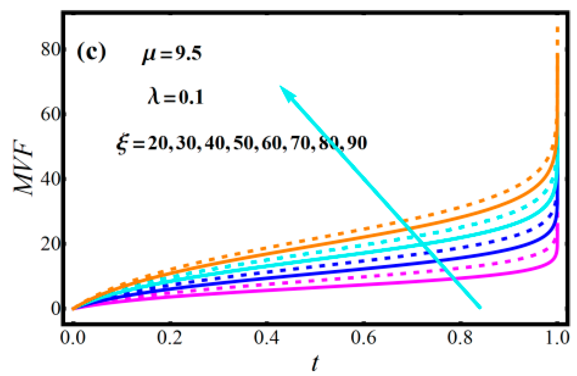
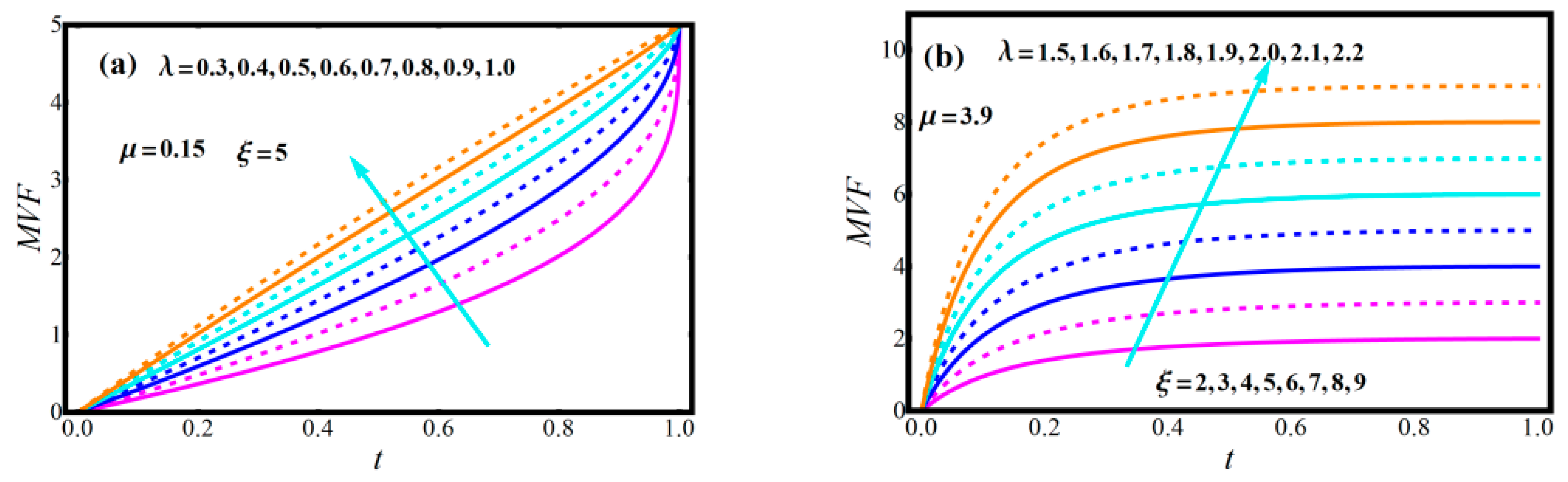
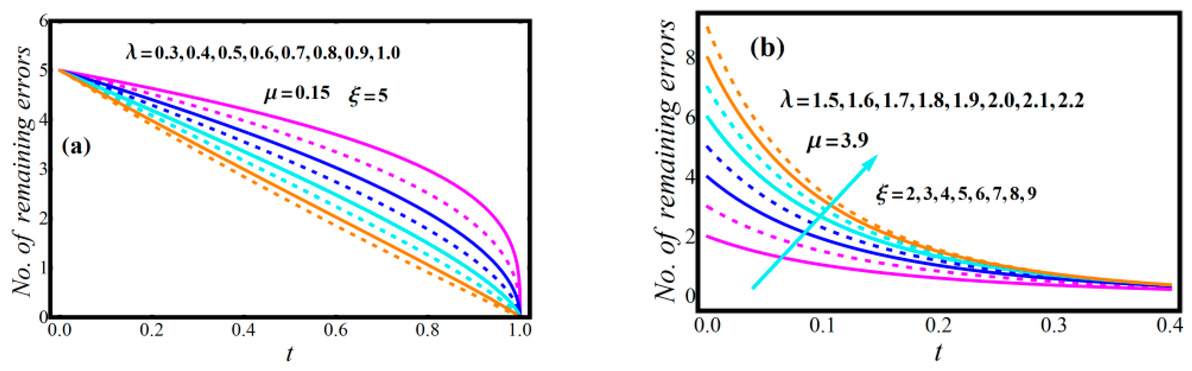
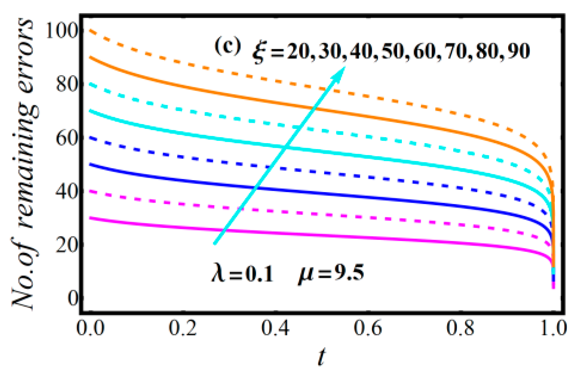
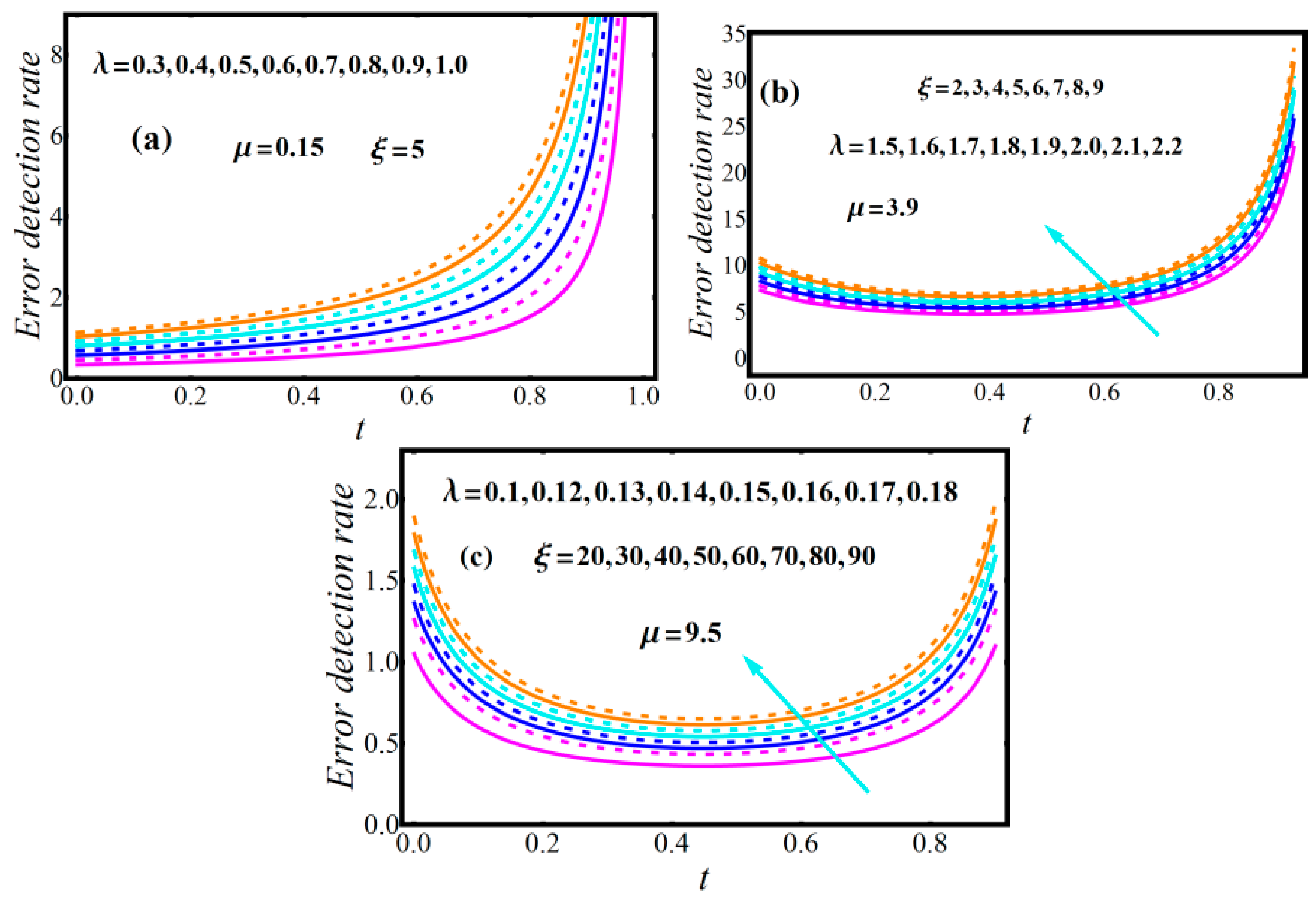
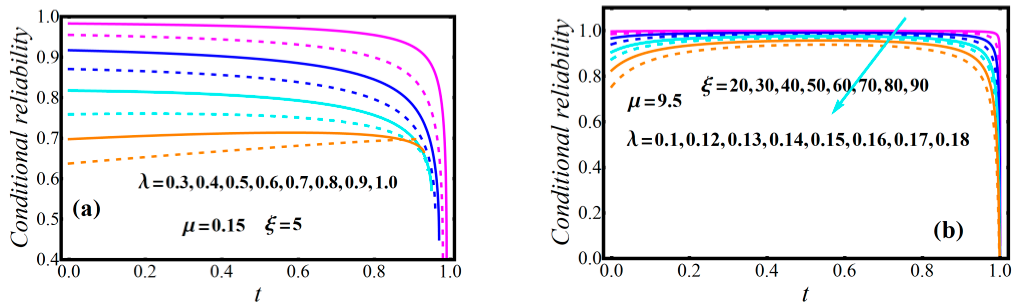
2.3. Diagrams of Model Attributes

Figure 1, Figure 2, Figure 3, Figure 4, Figure 5 and Figure 6 display the plots of the NHPP–NPF model’s features for various chosen input parameters. The MVF, which depicts the fluctuation in the number of errors identified with regard to time, is shown in Figure 1a–c. Defects found during testing were first quite high, but subsequently became steady. Greater values of parameter $\xi$ also generated a higher MVF form. Additionally, Figure 1 displays how the scale $\mu$ and shape $\lambda$ parameters evolved on the MVF profile. When $\mu \mathrm{and} \lambda >1,$ it produces a jump impact on the MVF profile, which decreased as $\mu <1 \mathrm{and} \lambda \le 1.$ Figure 2 illustrates how the intensity function (IF) changed across the various chosen parameters and had a high bathtub-shaped level with a greater value $\xi$ (see Figure 2c). The IF profile exhibits monotone growing (when $\mu , \lambda >1$) and declining ($\mu <1 \mathrm{and} \lambda \le 1$) behavior (see Figure 2a,b).

As the testing duration grew, the number of remaining error functions was reduced, as shown in Figure 3a–c; smaller values of parameter $\xi$ resulted in fewer appearances of the number of the remaining errors’ function. Figure 3b shows the behavior of $\mu \mathrm{and} \lambda$ on the number of the remaining errors functions’ profile.

Higher values ($\mu , \lambda >1$) of $\mu \mathrm{and} \lambda$ tended to enhance the profile of the remaining errors functions. When $\mu <1 \mathrm{and} \lambda \le 1$ and $\xi$ was constant, the profile of the remaining error functions was diminished. According to Figure 4a–c, the error detection rate function (EDRF) grew as testing duration grew; a higher value of the $\xi$ parameter resulted in bathtub shapes, which are desirable qualities in a lifetime model. When $\mu <1 \mathrm{and} \lambda \le 1$, $\xi$ was constant, and $\mu , \lambda >1,$ the EDRF increased as the testing period increased, resulting in a rising form of the failure occurrence rate per fault of the software function. These adaptable EDRF forms are great for including monotonic (MNT) and nonmonotonic (NMNT) EDRF trends that are typically present in practical applications. With the passage of testing time, the MTBF function profile in Figure 5a,b shows monotonic increasing behavior and bathtub shapes. Figure 6a,b shows that the conditional reliability approached zero as t increased to infinity.

$R\left(x|t\right)$ at different levels of $\lambda \mathrm{and} \xi$ demonstrates an initial rise to maximum and late fall to stationary of zero, at earlier time, most of the faults are yet removed; with elapsing time, more are debugged and this leads to a fall in software reliability; when the system is cleared of all faults, $R\left(x|t\right)$ reaches a stationary state. Therefore, later timeframe also presents a sharper drop to zero.

3. Estimation Techniques

The nonlinear least-squares (NLS), nonlinear weighted least-squares (NWLS), and maximum-likelihood (ML) techniques are employed in this section to estimate the parameters of the NHPP–NPF model.

NLSE, NWLSE and MLE Techniques

Suppose that, after T units of testing, n defects were found in the software system. Let $0<t_1<t_2<\dots$ $<t_n<T$ be the times when the failures were noticed. $\stackrel{⌣}{m}\left(t|\xi ,\lambda ,\mu \right)$ is the MVF with parameters $\xi ,\lambda$ and $\mu .$ The parameters were, thus, obtained from n observed data pairs: $\left({\stackrel{⌣}{m}}_0,t_0\right),\left({\stackrel{⌣}{m}}_1,t_1\right),$ $\dots ,\left({\stackrel{⌣}{m}}_n,t_n\right)$ where ${\stackrel{⌣}{m}}_i$ is the sum of all defects recorded throughout time $\left(0,t_i\right)$. The NLSE approach then needed to minimize the following function:

$$NLSE\left(\mathbf{t}|\xi ,\lambda ,\mu \right)={{\displaystyle \sum _{i=1}^n\left\{{\stackrel{⌣}{m}}_i-\stackrel{⌣}{m}\left(t_i|\xi ,\lambda ,\mu \right)\right\}}}^2={\displaystyle \sum _{i=1}^n{\left\{{\stackrel{⌣}{m}}_i-\xi \left(1-{\left(\frac{1-t_i}{1+\mu t_i}\right)}^{\lambda }\right)\right\}}^2},$$

(14)

Using (14) partial derivative $\left(\frac{\partial LSE\left(\mathbf{t}|.\right)}{\partial .}\right)$ with regard to $\xi ,\lambda \mathrm{and} \mu$, we obtain, respectively,

$$\frac{\partial LSE\left(\mathbf{t}|\xi ,\lambda ,\mu \right)}{\partial \xi }=-2{\displaystyle \sum _{i=1}^n\left\{{\stackrel{⌣}{m}}_i-\xi \left(1-{\left(\frac{1-t_i}{1+\mu t_i}\right)}^{\lambda }\right)\right\}}\left(1-{\left(\frac{1-t_i}{1+\mu t_i}\right)}^{\lambda }\right),$$

(15)

$$\frac{\partial LSE\left(\mathbf{t}|\xi ,\lambda ,\mu \right)}{\partial \mu }=-2\lambda \xi {\displaystyle \sum _{i=1}^n\frac{t_i{\left(\frac{1-t_i}{1+\mu t_i}\right)}^{\lambda }\left\{{\stackrel{⌣}{m}}_i-\xi \left(1-{\left(\frac{1-t_i}{1+\mu t_i}\right)}^{\lambda }\right)\right\}}{1+\mu t_i}},$$

(16)

$$\frac{\partial LSE\left(\mathbf{t}|\xi ,\lambda ,\mu \right)}{\partial \lambda }=2\xi {\displaystyle \sum _{i=1}^n{\left(\frac{1-t_i}{1+\mu t_i}\right)}^{\lambda }\ln \left(\frac{1-t_i}{1+\mu t_i}\right)\left\{{\stackrel{⌣}{m}}_i-\xi \left(1-{\left(\frac{1-t_i}{1+\mu t_i}\right)}^{\lambda }\right)\right\}}.$$

(17)

The WNLSE technique, on the other hand, needs to minimize the following function:

$$NWLSE\left(\mathbf{t}|\xi ,\lambda ,\mu \right)={\displaystyle \sum _{i=1}^n{\mathsf{\Theta }}_i{\left\{{\stackrel{⌣}{m}}_i-\stackrel{⌣}{m}\left(t_i|\xi ,\lambda , \mu \right)\right\}}^2},$$

(18)

$$WLS\left(\mathbf{t}|\xi ,\lambda ,\mu \right)={\displaystyle \sum _{i=1}^n{\mathsf{\Theta }}_i{\left\{{\stackrel{⌣}{m}}_i-\xi \left(1-{\left(\frac{1-t_i}{1+\mu t_i}\right)}^{\lambda }\right)\right\}}^2},$$

(19)

where ${\mathsf{\Theta }}_i>0,$ and $i=1,2,\dots ,n$ are positive weights ${\displaystyle \sum _{i=1}^n{\mathsf{\Theta }}_i=n}$ [39]. Using (19) partial derivative $\left(\frac{\partial LSE\left(\mathbf{t}|.\right)}{\partial .}\right)$ with regard to $\xi ,\lambda \mathrm{and} \mu$, we obtain, respectively,

$$\frac{\partial WLSE\left(\mathbf{t}|\xi ,\lambda ,\mu \right)}{\partial \xi }=-2{\displaystyle \sum _{i=1}^n{\mathsf{\Theta }}_i\left\{{\stackrel{⌣}{m}}_i-\xi \left(1-{\left(\frac{1-t_i}{1+\mu t_i}\right)}^{\lambda }\right)\right\}}\left(1-{\left(\frac{1-t_i}{1+\mu t_i}\right)}^{\lambda }\right),$$

(20)

$$\frac{\partial WLSE\left(\mathbf{t}|\xi ,\lambda ,\mu \right)}{\partial \mu }=-2\lambda \xi {\displaystyle \sum _{i=1}^n{\mathsf{\Theta }}_i\frac{t_i{\left(\frac{1-t_i}{1+\mu t_i}\right)}^{\lambda }\left\{{\stackrel{⌣}{m}}_i-\xi \left(1-{\left(\frac{1-t_i}{1+\mu t_i}\right)}^{\lambda }\right)\right\}}{1+\mu t_i}},$$

(21)

$$\frac{\partial LSE\left(\mathbf{t}|\xi ,\lambda ,\mu \right)}{\partial \lambda }=2\xi {\displaystyle \sum _{i=1}^n{\mathsf{\Theta }}_i{\left(\frac{1-t_i}{1+\mu t_i}\right)}^{\lambda }\ln \left(\frac{1-t_i}{1+\mu t_i}\right)\left\{{\stackrel{⌣}{m}}_i-\xi \left(1-{\left(\frac{1-t_i}{1+\mu t_i}\right)}^{\lambda }\right)\right\}}.$$

(22)

It is difficult to obtain the closed-form expression for the NLS and NWLS estimates of $\xi ,\lambda \mathrm{and} \mu .$ Therefore, parameter estimates can be obtained by numerically solving nonlinear Equations (15)–(17) and (20)–(22), and one can estimate $\stackrel{⌣}{m}\left(\mathbf{t}|\xi ,\lambda ,\mu \right)$ by substituting these estimates into Equation (5).

The log-likelihood function of the finite-failure NHPP model is obtained using (5) and (6) as follows.

$$l\left(\mathbf{t}|\xi ,\gamma ,\mu \right)=\log {\displaystyle \prod _{i=1}^n\frac{\xi \lambda \left(\mu +1\right){\left(1-t_i\right)}^{\lambda -1}}{{\left(1+\mu t_i\right)}^{\lambda +1}}\exp \left(-\xi \left\{1-{\left(\frac{1-t_n}{1+\mu t_n}\right)}^{\lambda }\right\}\right).}$$

(23)

$$l\left(\mathbf{t}|\xi ,\gamma ,\mu \right)=n\log \xi +n\log \lambda +n\log \left(\mu +1\right)+\left(\lambda -1\right){\displaystyle \sum _{i=1}^n\log \left(1-t_i\right)}-\left(\lambda +1\right){\displaystyle \sum _{i=1}^n\log \left(1+\mu t_i\right)}-\xi \left\{1-{\left(\frac{1-t_n}{1+\mu t_n}\right)}^{\lambda }\right\}.$$

(24)

Our objective was to obtain the MLEs. In order to do this, we first maximized (24), and computed partial derivatives with respect to unknown parameters and equal to zero in accordance with those results.

$$\frac{\partial l\left(\mathbf{t}|\xi ,\lambda ,\mu \right)}{\partial \xi }=\frac{n}{\xi }-\left\{1-{\left(\frac{1-t_n}{1+\mu t_n}\right)}^{\lambda }\right\},$$

(25)

$$\frac{\partial l\left(\mathbf{t}|\xi ,\lambda ,\mu \right)}{\partial \lambda }=\frac{n}{\lambda }+{\displaystyle \sum _{i=1}^n\log \left\{1-t_i\right\}}-{\displaystyle \sum _{i=1}^n\log \left(1+\mu t_i\right)}+\xi {\left(\frac{1-t_n}{1+\mu t_n}\right)}^{\lambda }\log {\left(\frac{1-t_n}{1+\mu t_n}\right)}^{\lambda },$$

(26)

$$\frac{\partial l\left(\mathbf{t}|\xi ,\lambda ,\mu \right)}{\partial \mu }=\frac{n}{1+\mu }-\xi \frac{\lambda t_n}{\left(1+\mu t_n\right)}{\left(\frac{1-t_n}{1+\mu t_n}\right)}^{\lambda }-{\displaystyle \sum _{i=1}^n\frac{\left(1+\lambda \right)t_i}{\left(1+\mu t_i\right)}}.$$

(27)

The final three nonlinear equations failed to yield the exact answers for MLEs and the ideal values of the estimates of $\xi ,\lambda \mathrm{and} \mu .$ MLEs could be evaluated numerically using statistical software [40].

4. Performance Evaluation

To study the effectiveness of our suggested models more, numerical experiments were conducted. The three techniques of estimation for the proposed model were compared using the illustrations of five real datasets. In order to compare the effectiveness of the suggested model with that of two other models, we also conducted comparative research. At the conclusion of this article, practical findings based on the real examined datasets are given and discussed. A software program that simplifies mathematical computation was created using Mathematica 12 and R language 3.6.1.

4.1. Failure Datasets

Five published datasets with different sizes were chosen for our evaluation study. References for the selected datasets are shown in Table 1.

4.2. Model Performance Measures

On the basis of (28)–(32), we utilized the following three criteria to assess how well the considered models performed. The discrepancy between the expected values and the actual observations is the mean square error (MSE), defined as follows:

$$MSE={\displaystyle \sum _{i=1}^n\left\{\frac{{\left({\stackrel{⌣}{m}}_i\left(t_i\right)-{\stackrel{⌢}{\stackrel{⌣}{m}}}_i\left(t_i\right)\right)}^2}{n-k}\right\}}$$

(28)

where n is the number of measurements, k is the number of parameters to be estimated, and ${\stackrel{⌣}{m}}_i\left(t_i\right)$ is the total cumulative number of errors seen in the range of times $\left(0,t_i\right)$. MVF ${\stackrel{⌢}{\stackrel{⌣}{m}}}_i\left(t_i\right)$ is the estimated cumulative number of errors at time $t_i$, obtained using the fitting mean value function. More trust in the model and hence better performance are indicated by a lower MSE score. The coefficient of determination ($R^2$) is defined as the difference between the sum of squares from the trend model and the constant model, and is defined as follows:

$$R^2=1-\frac{{\displaystyle \sum _{i=1}^n{\left({\stackrel{⌣}{m}}_i\left(t_i\right)-{\stackrel{⌢}{\stackrel{⌣}{m}}}_i\left(t_i\right)\right)}^2}}{{\displaystyle \sum _{i=1}^n{\left({\stackrel{⌣}{m}}_i\left(t_i\right)-{\stackrel{⌣}{m}}_i\left(t_i\right)/n\right)}^2}}.$$

(29)

$R^2\in \left[0,1\right]$ R calculates how much of the total variation is measured. The fitted curve is explained by the mean. The greater that $R^2$ is, the more effectively the model describes the data’s variation. Predictive validity [41] is the proportional discrepancy between the observed and estimated numbers of faults at time t. Predicted relative error (PRE) is

$$\mathrm{PRE}(t) =\frac{\stackrel{⌢}{\stackrel{⌣}{m}}\left(t\right)-\stackrel{⌣}{m}\left(t\right)}{\stackrel{⌣}{m}\left(t\right)} ,$$

(30)

where $\stackrel{⌢}{\stackrel{⌣}{m}}\left(t\right)$ and $\stackrel{⌣}{m}\left(t\right)$ are the estimated and observed faults determined at time t. Therefore, $\mathrm{PRE}(t) \to 0$ is sought for a better fit to the data [42]. Bias is the mean of the prediction errors (PEs). A prediction error is the sum of the prediction defects. Measures of the variance in the forecasts are frequently based on bias and its standard deviation.

$$\mathrm{Bias}={\displaystyle \sum _{i=1}^n\frac{PE\left(t_i\right)}{n}},$$

(31)

where $\mathrm{PE} \left(t_i\right)=\stackrel{⌢}{\stackrel{⌣}{m}}\left(t\right)-\stackrel{⌣}{m}\left(t\right).$

Predicted relative variation (PRV) is the term for the standard deviation of PRV [43]. Lower values of PRV and bias improve the quality of fit.

$$\mathrm{PRV}=\sqrt{\frac{{\displaystyle \sum _{i=1}^n{\left(PE\left(t_i\right)-\mathrm{Bias}\right)}^2}}{n-1}}.$$

(32)

The suggested software reliability model’s analytical algorithm is as follows.

• Under all approaches of estimation, the parameter estimates for the suggested model are estimated.
• Mean square error (MSE), the coefficient of determination (R²), predicted relative variation (PRV), and bias are calculated for effective model selection.
• The MVF of the suggested models is examined by comparing the estimation techniques.
• By examining the performance of the suggested model, research information on the ideal model is provided.

After analyzing the performance of the suggested model using the aforementioned techniques, we provide information on the model that software developers need.

Table 1. References for the datasets.

Dataset	References	Detected Failure
1	Hayakawa and Telfar [44]	30
2	Liu et al. [45]	15
3	Li and Pham, [45]	14
4	Wood [46]	20
5	Liu et al. [45]	17

Table 1. References for the datasets.

Dataset	References	Detected Failure
1	Hayakawa and Telfar [44]	30
2	Liu et al. [45]	15
3	Li and Pham, [45]	14
4	Wood [46]	20
5	Liu et al. [45]	17

5. Results and Discussion

We first utilized our framework to analyze how the suggested model behaved under various techniques and when using statistical data; then, we evaluated the software’s reliability.

5.1. Evaluation of the Estimation Techniques

On the basis of five datasets, this section assesses the effectiveness of the MLE, NLSE and WNLSE approaches for the NHPP–NPF model.

Table 2. Estimated values of parameters and assessment metrics of the NHPP–NPF model.

Dataset	Method of Estimation				Evaluation Criteria
		$\stackrel{⌣}{\mathit{\xi }}$	$\stackrel{⌣}{\mathit{\lambda }}$	$\stackrel{⌣}{\mathit{\mu }}$	MSE	𝑅-Squared	PRV	Bias
DS1	MLE	4.5742	1.9311	0.1297	0.0258	0.9160	0.2957	0.1429
	NLSE	2.7767	1.1877	1.8450	0.0132	0.5723	0.6538	0.3134
	WNLSE	2.7548	1.7996	1.7997	0.0012	0.9959	0.0602	0.0301
DS2	MLE	2.1665	2.5853	0.2602	0.0142	0.9373	0.2048	0.0963
	NLSE	1.7548	2.1456	1.5465	0.0024	0.9895	0.0849	0.0401
	WNLSE	1.7646	2.1458	1.5960	0.0012	0.9947	0.0597	0.0281
DS3	MLE	1.8977	0.7488	0.4875	0.0008	0.9820	0.0522	0.0250
	NLSE	1.8344	0.6999	0.9199	0.0003	0.9945	0.0279	−0.0132
	WNLSE	1.7910	0.7340	0.8923	0.0004	0.9922	0.0486	−0.0161
DS4	MLE	1.7814	1.6657	1.1161	0.0002	0.9941	0.0223	0.0107
	NLSE	1.7999	1.6999	1.1001	2.9 × 10−10	1.0000	3.1 × 10−5	1.4 × 10−5
	WNLSE	1.8001	1.6998	1.1000	3.4 × 10−10	1.0000	3.4 × 10−5	1.6 × 10−5
DS5	MLE	4.4177	1.2913	0.4699	0.0037	0.9642	0.1126	0.0545
	NLSE	3.7680	1.1952	1.0991	0.0001	0.9988	0.0202	0.0097
	WNLSE	3.7548	1.1752	1.0659	0.0015	0.9858	0.0695	0.0334

presents the outcomes. The values of the evaluation criteria in Table 2 led us to the following conclusions:

• The NHPP–NPF framework supports values that represent a more accurate model for the majority of the evaluation criteria in most situations when utilizing all three approaches.
• The outcomes of the many evaluation criteria varied, which suggests that it is necessary to research multiple criteria when comparing them.
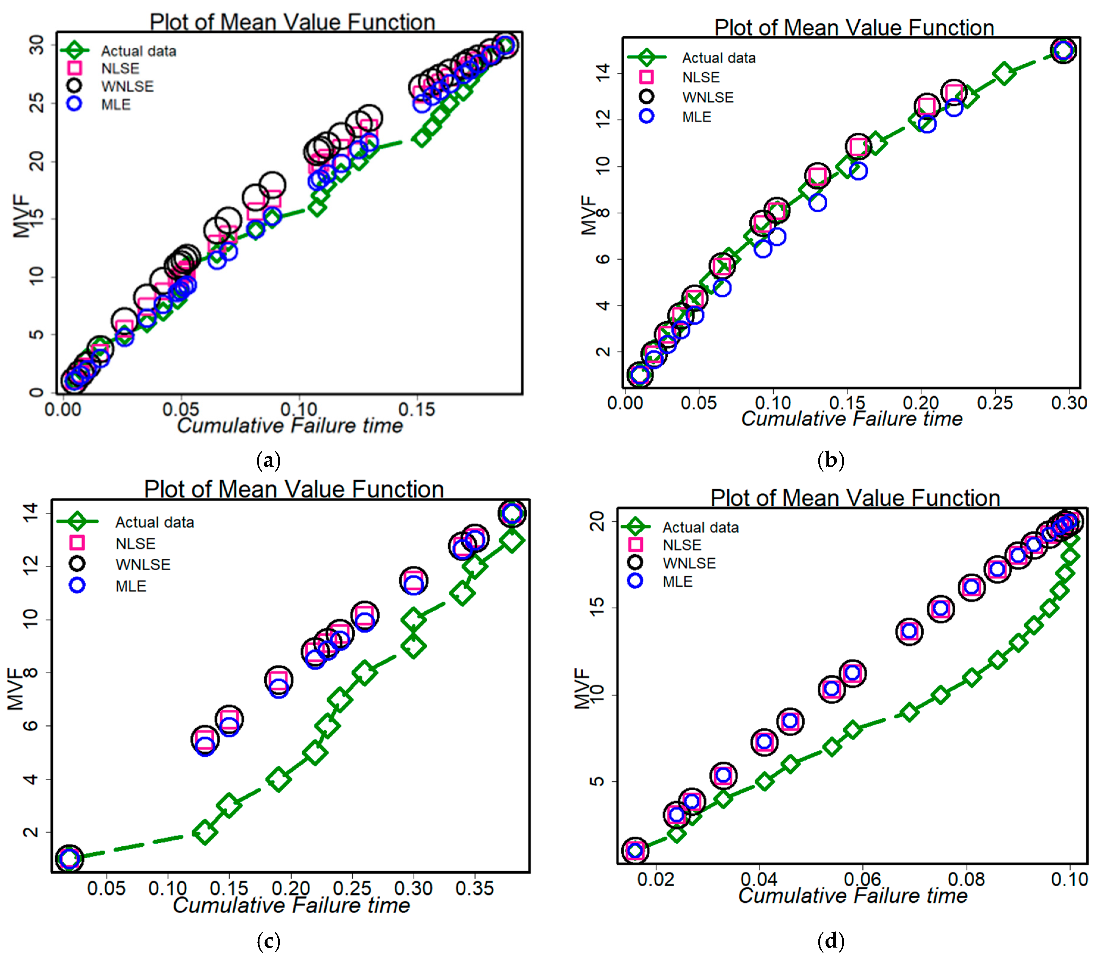
• The actual and fitted curves of software failures using the MLE, NLSE, and WNLSE approaches are shown in Figure 7a–e. These graphs show that our novel model, when applied to the MLE or WNLSE approaches, ensured that all datasets under consideration were well-fitted. In particular, when employing the WNLSE, NLSE, and MLE approaches, the suggested model was better suited for simulating the failure datasets. The suggested model, however, did not perform well when using the NLSE approach for DSI instead of the MLE and WNLSE methods.
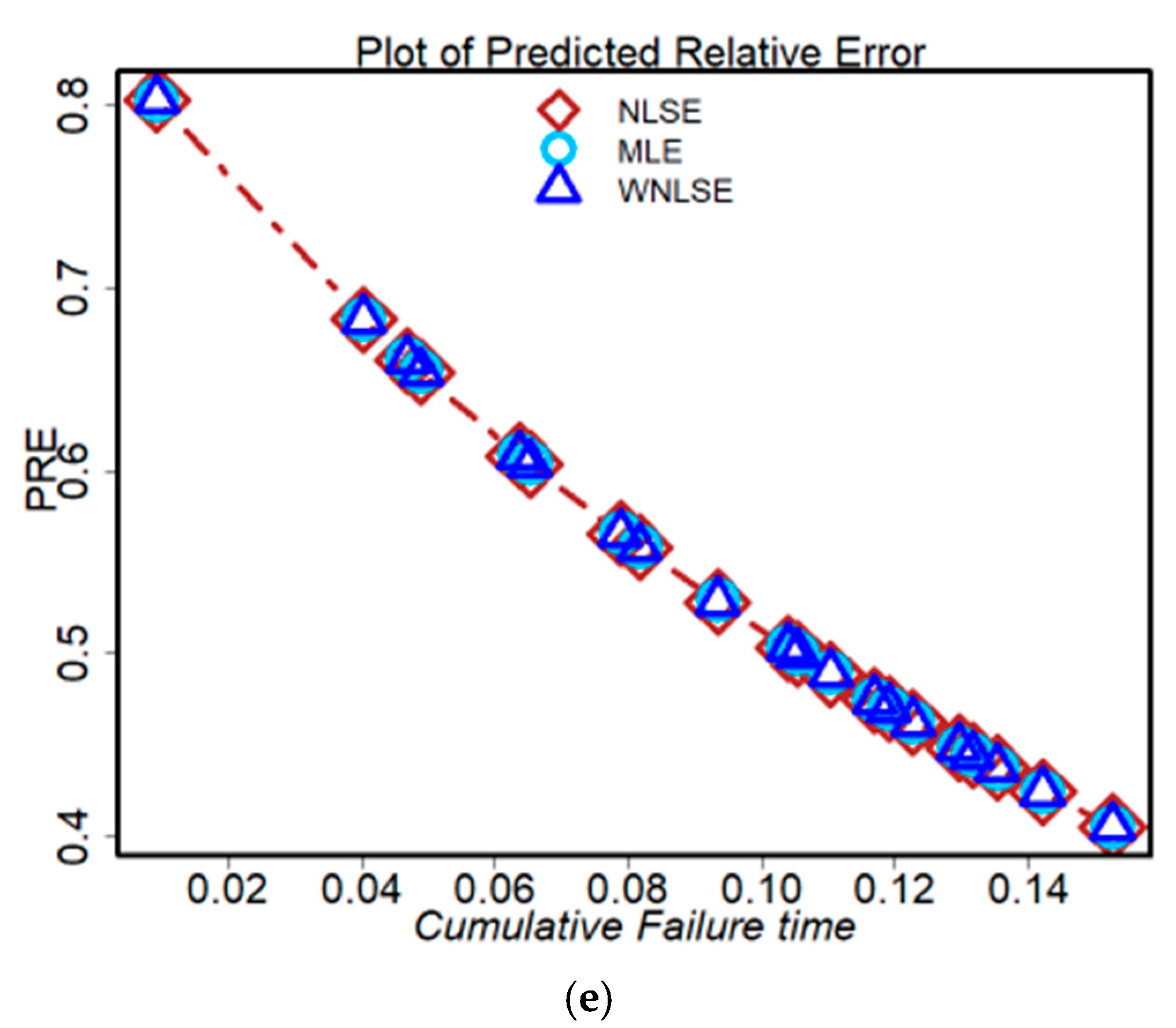
• Figure 8a–e shows the PRE outcomes for our NHPP–NPF model. The similarities among the three approaches may be seen in their early significant estimation error (deviation from zero) and later steadily moving toward observation. This was expected because there were initially few data that could be used to determine the parameters of the models; as time passed and more data became available, the models’ accuracy increased and their PRE decreased until it was zero.

5.2. Performance Evaluation of the SRGMs on Certain Real Datasets

We evaluated the accuracy of the suggested model, which is novel in terms of software reliability prediction and estimation with the SRGMs of NHPP power function Lehmann Type I (PFLI) and NHPP power function Lehmann Type II (PFLII), two benchmark PF models. The MLE was employed as the estimation method in our comparison analysis, which was based on five datasets.

Table 3. Results of model comparisons for various datasets.

Criteria	Dataset	PFLII	PFLI	NHPP–NPF
	DS1	0.0414	0.0938	0.0258
MSE	DS2	0.7098	0.0494	0.0132
	DS3	0.0445	0.2279	0.0008
	DS4	0.0342	0.0071	0.0002
	DS5	0.0774	0.0334	0.0037
𝑅-squared	DS1	0.9296	0.8135	0.9160
	DS2	0.6323	0.9355	0.9373
	DS3	0.8618	0.5218	0.9820
	DS4	0.8766	0.9873	0.9941
	DS5	0.8209	0.9372	0.9642
PRV	DS1	0.3570	0.5284	0.2957
	DS2	1.3944	0.3821	0.2048
	DS3	0.3820	0.8151	0.0522
	DS4	0.3398	0.1423	0.0223
	DS5	0.5135	0.3068	0.1126
Bias	DS1	0.1679	−0.2465	0.1429
	DS2	0.6323	−0.1765	0.0963
	DS3	0.1802	−0.3749	0.0250
	DS4	0.1622	−0.0654	0.0107
	DS5	0.2456	−0.1400	0.0545

presents the findings. We may see the following from the table:

• The MSE values for all investigated models were fairly similar; suggesting that all investigated models could accurately describe the five selected systems with just little variations in performance. The NHPP–NPF model ranked first for all datasets.
• The $R^2$ for all examined models was close to 1. As a result, all examined models are appropriate for modeling the software projects under consideration. The NHPP–NPF model positioned second for DSI, while it ranked first for DS2 to DS5.
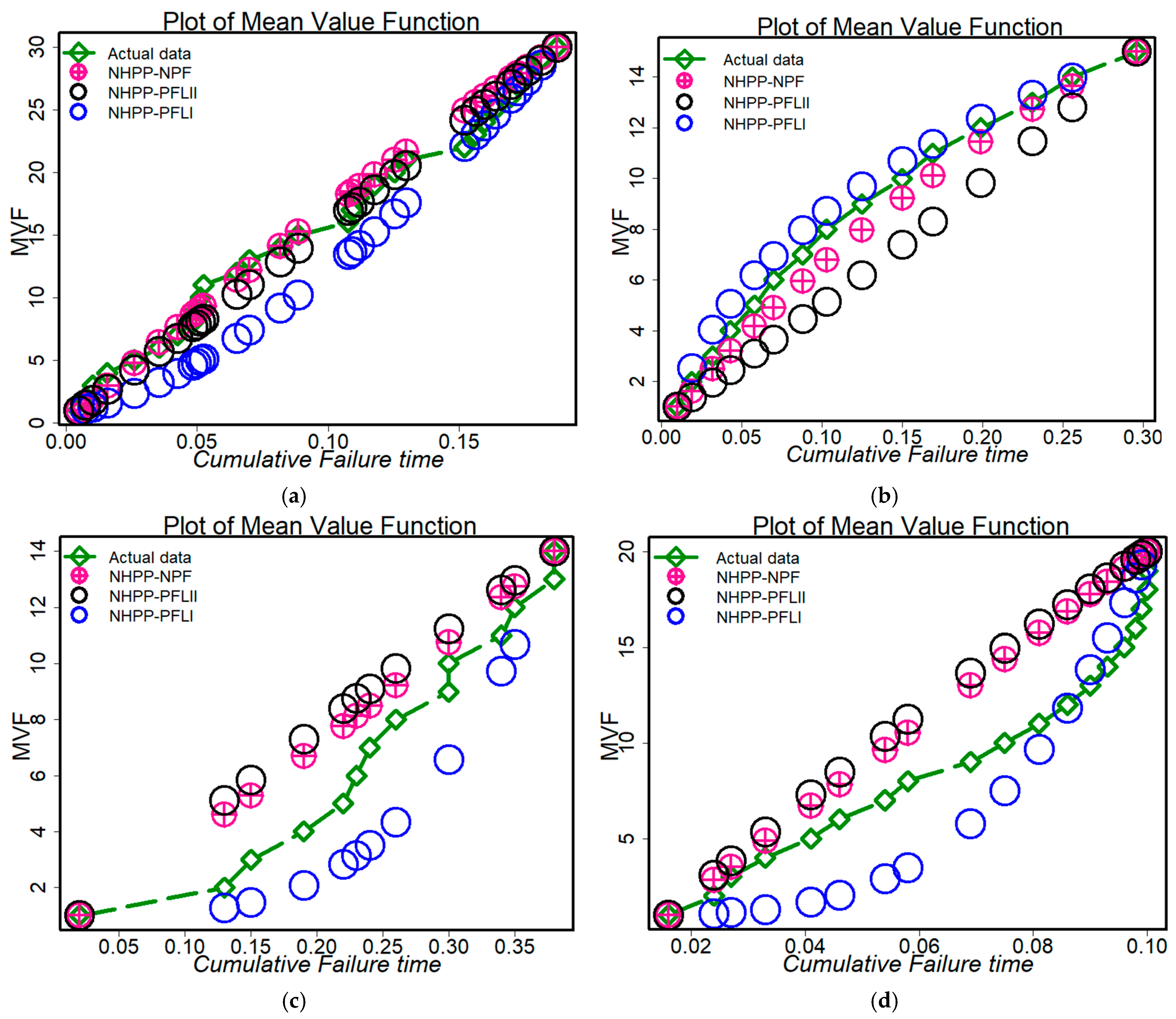
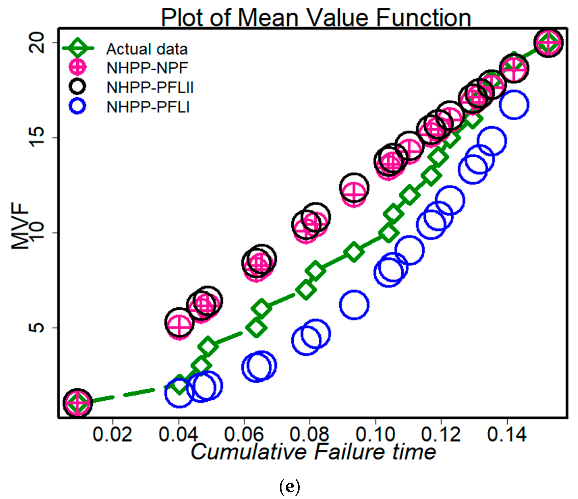
• Figure 9a–e shows the actual and predicted results depending on the four models under consideration. The figures demonstrate how well-fitted each of the chosen models was in analyzing the failure data. Specifically, the suggested model was among the best candidates for modeling the chosen datasets.

6. Conclusions

Using the NPF distribution as a foundation, we provided a novel reliability model in this work. Our proposed model, the NHPP–NPF model, has a number of crucial properties. Utilizing the NLSE, WNLSE, and MLE approaches, the model parameters under consideration were estimated. On the basis of eight datasets, various criteria were used to assess the performance of the estimators for each investigated approach. On the basis of five real datasets, a comparison study between the suggested model and two other models was carried out. All three approaches worked better for four different datasets, but the NLSE approach for the DSI failure dataset performed worse than WNLSE and MLE. Consequently, the WNLSE technique could be utilized with the NHPP types. In comparison to the other chosen models, the effectiveness of the NHPP–NPF model was positive. In the future, the present study could be extended by incorporating SRGMs with learning effects to increase the flexibility of models and to enhance their capability for accurately describing software failure phenomena.

References

1. Gokhale, S.S.; Lyu, M.R.; Trivedi, K.S. Software reliability analysis incorporating fault detection and debugging activities. In Proceedings of the Ninth International Symposium on Software Reliability Engineering (Cat. No. 98TB100257), IEEE, Paddeborn, Germany, 4–7 November 1998; pp. 202–211. [Google Scholar]
2. Xie, M. Software Reliability Modelling; World Scientific: Singapore, 1991; Volume 1. [Google Scholar]
3. Dalal, S.R.; Mallows, C.L. Some graphical aids for deciding when to stop testing software. IEEE J. Sel. Areas Commun. 1990, 8, 169–175. [Google Scholar] [CrossRef]
4. Zeephongsekul, P.; Xia, G.; Kumar, S. Software-reliability growth model: Primary-failures generate secondary-faults under imperfect debugging. IEEE Trans. Reliab. 1994, 43, 408–413. [Google Scholar] [CrossRef]
5. Jones, W.D. Reliability models for very large software systems in industry. In Proceedings of the 1991 International Symposium on Software Reliability Engineering, IEEE Computer Society, Austin, TX, USA, 17–18 May 1991; pp. 35–36. [Google Scholar]
6. Pham, H. Software Reliability; Springer Science & Business Media: Berlin/Heidelberg, Germany, 2000. [Google Scholar]
7. Kapur, P.K.; Kumar, S.; Garg, R.B. Contributions to Hardware and Software Reliability; World Scientific: Singapore, 1999; Volume 3. [Google Scholar]
8. Gokhale, S.S. Architecture-based software reliability analysis: Overview and limitations. IEEE Trans. Dependable Secur. Comput. 2007, 4, 32–40. [Google Scholar] [CrossRef]
9. Wang, W.L.; Hemminger, T.L.; Tang, M.H. A moving average non-homogeneous Poisson process reliability growth model to account for software with repair and system structures. IEEE Trans. Reliab. 2007, 56, 411–421. [Google Scholar] [CrossRef]
10. Kapur, P.K.; Xie, M.; Garg, R.B.; Jha, A.K. A discrete software reliability growth model with testing effort. In Proceedings of the 1994 1st International Conference on Software Testing, Reliability and Quality Assurance (STRQA’94), IEEE, New Delhi, India, 21–22 December 1994; pp. 16–20. [Google Scholar]
11. Kapur, P.K.; Younes, S.; Agarwala, S. A general discrete software reliability growth model. Int. J. Model. Simul. 1998, 18, 60–65. [Google Scholar] [CrossRef]
12. Schneidewind, N.F. Analysis of error processes in computer software. In Proceedings of the International Conference on Reliable Software, Los Angeles, CA, USA, 21–23 April 1975; pp. 337–346. [Google Scholar]
13. Xie, M.; Zhao, M. On some reliability growth models with simple graphical interpretations. Microelectron. Reliab. 1993, 33, 149–167. [Google Scholar] [CrossRef]
14. Song, K.Y.; Chang, I.H.; Pham, H. A software reliability model with a Weibull fault detection rate function subject to operating environments. Appl. Sci. 2017, 7, 983. [Google Scholar] [CrossRef]
15. Kim, H.-C.; Sebuk-gu, S.-e.; Chungcheongnam-do, C.-s. Assessing software reliability based on NHPP using SPC. Int. J. Softw. Eng. Its Appl. 2013, 7, 61–70. [Google Scholar]
16. Park, S.K. A Comparative Study on the Attributes of NHPP Software Reliability Model Based on Exponential Family and Non-Exponential Family Distribution. J. Theor. Appl. Inf. Technol. 2021, 99, 5735–5747. [Google Scholar]
17. Xu, J.; Yao, S. Software reliability growth model with partial differential equation for various debugging processes. Math. Probl. Eng. 2016, 2016, 2476584. [Google Scholar] [CrossRef]
18. Al-Mutairi, N.N.; Al-Turk, L.I.; Al-Rajhi, S.A. A New Reliability Model Based on Lindley Distribution with Application to Failure Data. Math. Probl. Eng. 2020, 2020, 4915812. [Google Scholar] [CrossRef]
19. Dohi, X.X.T. On the role of Weibull-type distributions in NHPP-based software reliability modeling. Int. J. Perform. Eng. 2013, 9, 123. [Google Scholar]
20. Pham, H. Distribution Function and its Applications in Software Reliability. Int. J. Perform. Eng. 2019, 15, 1306. [Google Scholar] [CrossRef]
21. Kim, H.-C. A Study on Comparative Evaluation of Software Reliability Model According to Learning Effect of Exponential-exponential Distribution. Int. J. Eng. Res. Technol. 2020, 3043–3047. [Google Scholar] [CrossRef]
22. Hui, Z.; Liu, X. Research on software reliability growth model based on Gaussian new distribution. Procedia Comput. Sci. 2020, 166, 73–77. [Google Scholar] [CrossRef]
23. Tae-Jin, Y. A Study on the Reliability Performance Analysis of Finite Failure NHPP Software Reliability Model Based on Weibull Life Distribution. Int. J. Eng. Res. Technol. 2019, 12, 1890–1896. [Google Scholar]
24. Yang, T.J. A Comparative study on the Cost and Release Time of Software Development Model Based on Lindley-Type Distribution. Int. J. Eng. Res. Technol. 2020, 13, 2185–2190. [Google Scholar] [CrossRef]
25. Kim, H.C.; Moon, S.C. A Study on the Reliability Performance Evaluation of Software Reliability Model Using Modified Intensity Function. J. Inf. Technol. Appl. Manag. 2018, 25, 109–116. [Google Scholar]
26. Kim, H.C.; Shin, H.C. The Comparative Study of NHPP Software Reliability Model Based on Exponential and Inverse Exponential Distribution. J. Korea Inst. Inf. Electron. Commun. Technol. 2016, 9, 133–140. [Google Scholar] [CrossRef]
27. Li, S.; Dohi, T.; Hiroyuki, O. Burr-type NHPP-based software reliability models and their applications with two type of fault count data. J. Syst. Softw. 2022, 191, 111367. [Google Scholar] [CrossRef]
28. Dallas, A. 1. lntroduction Let X be a random variable with distribution function. Ann. Inst. Stat. Math. 1976, 28, 491–497. [Google Scholar] [CrossRef]
29. Meniconi, M.; Barry, D.M. The power function distribution: A useful and simple distribution to assess electrical component reliability. Microelectron. Reliab. 1996, 36, 1207–1212. [Google Scholar] [CrossRef]
30. Tavangar, M. Power function distribution characterized by dual generalized order statistics. J. Iran. Stat. Soc. 2011, 10, 13–27. [Google Scholar]
31. Chang, S.K. Characterizations of the power function distribution by the independence of record values. J. Chungcheong Math. Soc. 2007, 20, 139–146. [Google Scholar]
32. Cordeiro, G.M.; dos Santos Brito, R. The beta power distribution. Braz. J. Probab. Stat. 2012, 26, 88–112. [Google Scholar]
33. Tahir, M.H.; Alizadeh, M.; Mansoor, M.; Cordeiro, G.M.; Zubair, M. The Weibull-power function distribution with applications. Hacet. J. Math. Stat. 2016, 45, 245–265. [Google Scholar] [CrossRef]
34. Jabeen, R.; Zaka, A. Estimation of parameters of the continuous uniform distribution: Different classical methods. J. Stat. Manag. Syst. 2020, 23, 529–547. [Google Scholar] [CrossRef]
35. Butt, N.S.; ul Haq, M.A.; Usman, R.M.; Fattah, A.A. Transmuted power function distribution. Gazi Univ. J. Sci. 2016, 29, 177–185. [Google Scholar]
36. Iqbal, M.Z.; Arshad, M.Z.; Özel, G.; Balogun, O.S. A better approach to discuss medical science and engineering data with a modified Lehmann Type II model. F1000 Res. 2021, 10, 823. [Google Scholar] [CrossRef]
37. Yamada, S.; Ohba, M.; Osaki, S. S-shaped reliability growth modeling for software error detection. IEEE Trans. Reliab. 1983, 32, 475–484. [Google Scholar] [CrossRef]
38. Chiu, K.C.; Huang, Y.S.; Lee, T.Z. A study of software reliability growth from the perspective of learning effects. Reliab. Eng. Syst. Saf. 2008, 93, 1410–1421. [Google Scholar] [CrossRef]
39. Ishii, T.; Dohi, T.; Okamura, H. Software reliability prediction based on least squares estimation. Qual. Technol. Quant. Manag. 2012, 9, 243–264. [Google Scholar] [CrossRef]
40. Sindhu, T.N.; Atangana, A. Reliability analysis incorporating exponentiated inverse Weibull distribution and inverse power law. Qual. Reliab. Eng. Int. 2021, 37, 2399–2422. [Google Scholar] [CrossRef]
41. Zhao, J.; Liu, H.W.; Cui, G.; Yang, X.Z. Software reliability growth model with change-point and environmental function. J. Syst. Softw. 2006, 79, 1578–1587. [Google Scholar] [CrossRef]
42. Pillai, K.; Nair, V.S. A model for software development effort and cost estimation. IEEE Trans. Softw. Eng. 1997, 23, 485–497. [Google Scholar] [CrossRef]
43. Hayakawa, Y.; Telfar, G. Mixed poisson-type processes with application in software reliability. Math. Comput. Model. 2000, 31, 151–156. [Google Scholar] [CrossRef]
44. Liu, J.; Liu, Y.; Xu, M. Parameter estimation of Jelinski-Moranda model based on weighted nonlinear least squares and heteroscedasticity. arXiv arXiv preprint. 2015, arXiv:1503.00094. [Google Scholar]
45. Li, Q.; Pham, H. NHPP software reliability model considering the uncertainty of operating environments with imperfect debugging and testing coverage. Appl. Math. Model. 2017, 51, 68–85. [Google Scholar] [CrossRef]
46. Wood, A. Predicting software reliability. Computer 1996, 29, 69–77. [Google Scholar] [CrossRef]
Figure 1. Visualization of the MVF of the NHPP–NPF model.
Mathematics 11 00842 g001aMathematics 11 00842 g001b
Figure 2. Visualization of the intensity function of the NHPP–NPF model.
Mathematics 11 00842 g002
Figure 3. Plots of the number of remaining faults’ function of the NHPP–NPF model.
Mathematics 11 00842 g003aMathematics 11 00842 g003b
Figure 4. Plots of the error detection rate function of the NHPP–NPF model.
Mathematics 11 00842 g004
Figure 5. Plots of the MTBF function of the NHPP–NPF model.
Mathematics 11 00842 g005
Figure 6. Plots of the conditional reliability of the NHPP–NPF model.
Mathematics 11 00842 g006
Figure 7. Comparison of the estimating techniques for the NHPP–NPF model for (a) DS1, (b) DS2, (c) DS3 (d) DS4, and (e) DS5. (left to right).
Mathematics 11 00842 g007aMathematics 11 00842 g007b
Figure 8. PRE for the estimating techniques for NHPP–NPF compared with five datasets: (a) DS1, (b) DS2, (c) DS3 (d) DS4, and (e) DS5.
Mathematics 11 00842 g008aMathematics 11 00842 g008b
Figure 9. Observed and predicted results with five datasets: (a) DS1, (b) DS2, (c) DS3 (d) DS4, and (e) DS5.
Mathematics 11 00842 g009aMathematics 11 00842 g009b