Vehicle Routing Optimization with Cross-Docking Based on an Artificial Immune System in Logistics Management

Abstract

Background: Manufacturing companies optimize logistics network routing to reduce transportation costs and operational costs in order to make profits in an extremely competitive environment. Therefore, the efficiency of logistics management in the supply chain and the quick response to customers’ demands are treated as an additional source of profit. One of the warehouse operations for intelligent logistics network design, called cross-docking (CD) operations, is used to reduce inventory levels and improve responsiveness to meet customers’ requirements. Accordingly, the optimization of a vehicle dispatch schedule is imperative in order to produce a routing plan with the minimum transport cost while meeting demand allocation. Methods: This paper developed a two-phase algorithm, called sAIS, to solve the vehicle routing problem (VRP) with the CD facilities and systems in the logistics operations. The sAIS algorithm is based on a clustering-first and routing-later approach. The sweep method is used to cluster trucks as the initial solution for the second phase: optimizing routing by the Artificial Immune System. Results: In order to examine the performance of the proposed sAIS approach, we compared the proposed model with the Genetic Algorithm (GA) on the VRP with pickup and delivery benchmark problems, showing average improvements of 7.26%. Conclusions: In this study, we proposed a novel sAIS algorithm for solving VRP with CD problems by simulating human body immune reactions. The experimental results showed that the proposed sAIS algorithm is robustly competitive with the GA on the criterion of average solution quality as measured by the two-sample t-test.

1. Introduction

The concept of a smart city includes a high degree of information technology (IT) integration and communication, which is the same concept as supply chain management today, which relies on the use of various ITs and techniques. One of the important elements of smart cities is smart logistics, aiming to help manufacturers gain performance from reusable transport packaging, such as pallets, racks, and bins, as well as tracking packages. By building Internet of Things (IoT) monitoring technology, smart logistics IT systems can be integrated into virtually any transportation asset to track its location in real-time, optimize inventory planning, and monitor environmental conditions, especially when the world enters the fifth-generation mobile communication technology or even the six-generation mobile communication technology in the future [1,2,3]. However, even with advanced IT today, logistics costs are still an important part of a global company’s worldwide operation management to construct an enterprise’s competitive edge over competitors, especially when dealing with post-COVID-19 supply chain disruptions. Intelligent logistics network functions allow companies to quickly respond to customer requirements and create their own competitive advantage over competitors in the design of smart logistics by using IT, such as radio frequency identification, to track shipments in real-time. Moreover, logistics costs weigh significantly on a company’s total costs. The authors of [4] identified the logistics costs from three different aspects of a case company: (1) the share of procurement costs reduced from approximately 0.65 (2013) to 0.45% (2015); (2) the share of production costs increased from approximately 50 (2013) to 65% (2015); and (3) the share of sales costs increased from approximately 7 (2013) to 8.5% (2015). As a result, in order to increase overall profits, lower operational costs, and improve a company’s service level, a well-designed and highly cost-efficient logistics mechanism becomes essential. The paper focuses on controlling transport costs by optimizing routes and scheduling of vehicles, which is known as the vehicle routing problem (VRP) [5].

VRPs are a fundamental activity in the fields of transportation systems, distribution channel design, and logistics networks. The study of the VRPs is indeed vital in optimizing the physical flow of goods in the logistics operation in order to reduce transport costs and increase supply chain network performance. Among numerous studies of the VRPs, the problem with optimal routes and scheduling of vehicles, considering both pickup and delivery processes simultaneously, is called the VRP with cross-docking (VRPCD). Kulwiec (2004) pointed out that the cross-docking (CD) facility is an important supply chain strategy. They classified the CD facility into six different types. One of the CD operations is “Truck/Rail Consolidation.” [6]. Both suppliers’ and retailers’ sides of the supply chain have to be considered at the same time in the process of transporting goods. Therefore, CD facilities are an important element in a synchronized supply chain as well as in sustainable logistics management. Generally, there would be no interruption between upstream and downstream operations as long as the physical flow of goods in the pickup process is simultaneously delivered at the CD depot and then delivered to customers after the consolidation process. Therefore, no inventory was stocked, and no delay in customer orders occurred at the facility. As a result, the construction of a CD system in the logistics network makes companies able to: (1) facilitate the efficiency and effectiveness of supply chain management; (2) lower space requirements and reduce transportation costs; and (3) better control the distribution process [7]. Figure 1 shows a simple layout of the CD depot.

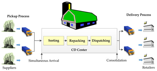
Figure 1. A layout of a typical CD facility.

Studying an efficient heuristics methodology is essential to acquiring an optimal or near-optimal solution within a reasonable amount of computation time because the VRP is a well-known non-deterministic polynomial-time-hard (NP-hard) problem. As the global pandemic of the new coronavirus (COVID-19) has shaken the world since 2020, the study of the human immune system has piqued the interest of many researchers. The Artificial Immune Systems (AIS) is the simulation algorithm of human body defense systems and is applied to solve many research fields, such as clustering/classification, fault detection, combinatorial optimization, and learning problems [8,9,10,11,12].

The AIS has presented numerous studies on solving optimization problems. The results showed that their algorithm was a feasible and effective method for the VRP. For example, the authors of [13] applied clonal selection to tackle the VRP by using clonal selection operators, super mutation operators, and clonal proliferation to improve global convergence speed. The results indicate that their algorithm has a remarkable reliability of global convergence and avoids prematurity when solving the VRP effectively.

This paper aims to propose a two-phase optimization approach based on an artificial immune system combined with the sweep method, called sAIS, to solve the vehicle routing problem with the CD facilities in the logistics network as an important element of smart city infrastructure. The two-phase approach begins with the grouping method to fulfill vehicle capacity constraints and is followed by the optimization engine to find near-optimal solutions for each truck routing sequence while utilizing a minimum number of trucks. The experimental results showed that the proposed sAIS algorithm is robustly competitive with the GA on the criterion of average solution quality.

The remainder of this paper is organized as follows. Section 2 reviews the related literature, and Section 3 defines the VRPCD formulation. Section 4 details the methodology and procedure of our proposed sAIS heuristic algorithm, following a number of experimentation examples presented in Section 5. Section 6 concludes the research with a summary based on the computational results.

2. Related Works

The CD system is a lean supply chain model of transporting raw materials or products from pickup to delivery without ever storing them in the warehouse. It can significantly reduce inventory levels, required space, handling costs, and lead times, as well as customer response times. Packages are unloaded from inbound trucks immediately after arriving at the depot, followed by a sorting, repacking, and dispatching process as shown in Figure 2, then loaded onto outbound trucks for delivery to retailers in a distribution channel [14,15,16,17,18]. The primary objective is to avoid a high inventory level and reduce handling costs so that there will be no inventory being stored in the depot. This is the same concept as the Toyota Production System or lean operations. A well-designed CD operation can provide companies with significant benefits, including decreased inventory levels, low storage space requirements, low transportation costs, a fast response to customer requirements, and better control of the distribution process. Both receiving and shipping processes must be considered simultaneously, to enable the CD facility to be integrated into the logistics network effectively. Lee, Jung, and Lee (2006) first proposed that the most important process for CD operations is the pickup phase, in which all trucks must arrive at the depot at the same time in order to control the start time of warehouse operations [17].

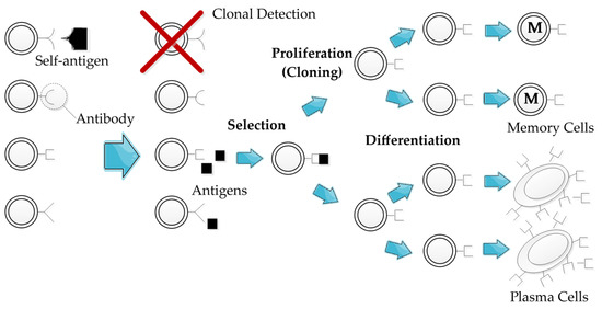
Figure 2. The selection process of antibodies.

Before the CD system served as a mathematical constraint, Dantzig and Ramaser (1959) initially introduced the VRP concept as a solution to the “Truck Dispatching Problem.” In their study, a linear programming model was designed to acquire a near-best solution for the truck scheduling problem, which was concerned with the optimum routing of a fleet of delivery trucks supplied by the terminal [19]. Following that, numerous research proposals were made to address the developing VRPs in their study. The VRPs have been studied for many decades. The VRP is a set of customers with known demands who are serviced by a fleet of trucks from one or more depots to a number of geographically dispersed locations and customers based on optimally designed routes [20,21,22,23,24].

There are many solving methods for variants of the VRP proposed in the literature. The authors of [25] dealt with capacitated VRP and distance restrictions by using an integer programming method that used a constraint relaxation approach and sub-tour elimination. The author of [26] proposed tour-partitioning heuristics to solve the pickup and delivery VRPs, whereas the authors of [27] developed a hybrid heuristic method based on the Genetic Algorithm (GA) with neighborhood search to solve the basic VRPs. They showed that the hybrid GA had a significant improvement over the pure GA and was competitive with the simulated annealing approach [28] and the Tabu search approach [29,30,31] in their experiment results. The authors of [32,33] proposed hybrid ant colony optimizations (ACOs) to solve the VRPs with time windows and found that they were applicable and effective in practical problems. The authors of [34] used an ACO approach for the multiple VRPs with pickup and delivery along with time windows and heterogeneous fleets and applied it to large-scale problems. The authors of [18] developed a matheuristic approach consisting of two phases: adaptive large neighborhood search (ALNS) and setting partitioning to solve VRPCD. The authors of [35] proposed a particle swarm optimization approach to solve VRPCD and carbon emissions reduction. Moreover, sustainable logistics management is a popular research topic nowadays to follow the United Nations’ sustainable development goals [36].

Following the same concept to simulate an ant’s behavior as ACO, Jerne (1974) proposed the first AIS model to simulate the immune system as a mathematical formulation to solve optimization problems, which had an interaction network of lymphocytes and molecules that had variable regions [37]. Following Jerne’s research, Farmer, Packard, and Perelson (1986) proposed the dynamic immune network, which could simulate and solve classification problems, showing the AIS can be extended to solve big data prediction problems nowadays as machine learning pioneers [38]. Kephart (1994) published a paper on the AIS from a biological point of view to auto-distinguish computer viruses [39]. Hunt et al. (1999) devoted themselves to developing clonal selection algorithms and proposing high-frequency variations [40]. Lately, Mrowczynska et al. (2017) used AIS to predict road freight transportation [41]. Mabrouk, Raslan, and Hedar (2022) proposed an immune system programming with local search (ISPLS) algorithm with a tree data structure to be used in the meta-heuristics programming approach to develop new practical machine learning tools [42]. As a result of many years of development, the AIS has become a well-known meta-heuristic that is widely applied to solve combinatorial optimization and abnormal detection problems.

The AIS mainly simulates the relationship between antigens and antibodies, and the core idea of immune reactions includes antibodies’ reproduction, clonal expansion, and immune memory properties in the biological immune system. Organisms have two kinds of immunity: the innate immune system and the adaptive immune system. The innate immune system is capable of recognizing molecular patterns in pathogens and signaling other immune cells to start fighting against the pathogens. Adaptive immune systems can maintain a stable memory of known patterns. Living organisms use the immune system to defend their bodies from invasion by outside substances. Lymphocytes are parts of the immune system, which includes T and B cells. Both types of lymphocytes have surface receptors capable of recognizing molecular patterns present on antigens (binding with epitopes). When the receptors bind to epitopes and exceed a threshold, a lymphocyte becomes activated.

Activation triggers a series of reactions that can lead to the elimination of pathogens. During the infection response, the immune system’s B cells produced antibodies. Pathogens are bound by antibodies called antigens. Antigens and antibodies can bind together when complementary shapes exist. After binding, the antibody disables the pathogens so that the immune system can easily destroy them. Figure 2 depicts how to select immune system antibodies [43,44,45,46].

There are four types of immune mutations running inside the human body: IgM, IgG, IgE, and IgA [47,48,49,50]. In this paper, we simulate each mode having a different mathematical function. First, the calculation of affinity is the total correlations between the antigen-antibodies and antibodies-antibodies in our mathematical programming model. If the affinity value of a new string in IgM mode is smaller than that of the old one, a total of four kinds of immune mutations, including IgG mode, IgE mode, and IgA mode, are randomly selected to operate in the next step of mutation in the same generation for optimization purposes.

• Somatic Hypermutation Simulation Function:
  • IgM mode: Inverse mutation is used in the IgM mode. In the sequence s, randomly selected two positions, i and j. Inverse the sequence of cells between the i and j positions in the neighbor of s. It should be noted if |i − j| < 2 it cannot be mutated;
  • IgG mode: Pairwise mutation is used in the IgG mode. In the sequence s, randomly selected two positions, i and j. Swap these two cells in the neighbor of s;
  • IgA mode: Insertion mutation is used in the IgA mode. In the sequence s, randomly selected two positions, i and j. Insert the cell i to the position j in the neighbor of s;
  • IgE mode: Both the swap and insertion mutations are used in the IgE mode. In the sequence s, randomly selected two positions, i and j. A new sequence s’ is provided by swapping i and j. Then, in the sequence, s’ randomly selected i’ and j’ to be a cell and a position, respectively. Inserting cell i at position j in the neighbor of s’.
• Affinity Maturation Simulation Function

Affinity is a positive or negative correlation between an antigen and an antibody. When the affinity is higher, it can generate a better fit between the interacting surfaces of the antibody and antigen. After somatic hypermutation, some variant antibodies with higher affinities may be produced. Then, in the next response, the cells will have a greater affinity. This phenomenon is called affinity maturation;

3.

Elimination Simulation Function

The human body’s bone marrow generates billions of B cells into circulation every day. Those B cells are saved in a catalog, where there is limited storage space for the B cells. The B cells are dead within a certain period if they meet the specific antigen. Hence, the B-cell catalog is not static, and newly produced antibodies are continually tested against antigen infection. Therefore, new antibodies are generated and old ones are deleted.

3. VRPCD Formulation

The VRP is traditionally illustrated as a graph network with vertices denoting terminal points and arcs as vehicle routes, as shown in Figure 3. The basic notations for all VRPs are shown as follows:

G = (V, E ∪ A),

where V = {v₀, …, v_n} is a vertex set; v₀ represents the central warehouse from which deliveries are made;

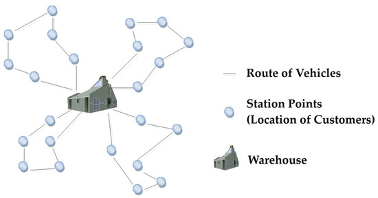
Figure 3. A simple illustration of the VRP routing network.

A = {(v_i, v_j): i ≠ j, v_i, v_j ∈ V} represents the directed arc set;

E = {(v_i, v_j): i < j, v_i, v_j ∈ V} is a set of undirected edges.

Lee, Jung, and Lee (2006) addressed the constraints of vehicle routing with the one CD warehouse problem. The CD facility plays a key role in synchronizing the distribution process on both sides of the supply chain [17]. As simulated, the CD facility can be treated as the home depot as in the traditional VRPs, except that the model of CD specifies the simultaneous arrival of each vehicle from the receiving trip. Therefore, several assumptions are made. First, we have n nodes, denoting a total number of suppliers and retailers, who are serviced by m vehicles. Every truck must depart and come back to the depot (i = 0), with the simultaneous arrival of trucks from pickup routes. Second, for each customer, only one truck is assigned and associated with a cost amount of C_ij. Every customer has a homogeneous demand d, which is related to the capacity limit q_k for truck k. Additionally, a constraint of the planning time horizon T specifies that the total distance traveled by vehicles cannot exceed it. Two types of costs are considered: transportation costs and operational costs. The objective of this research in the mathematical programming model is to find optimized routing solutions by using a minimum number of trucks to service and complete the assignment. The following presents the basic notations of the VRPCD model.

Decision Variables:

X_ijk: a binary variable representing the route from i to j is serviced by vehicle k, where $X_{ijk}=\{\begin{array}{ll}1,\hfill & \mathrm{if} \mathrm{vehicle} k \mathrm{is} \mathrm{in} \mathrm{the} \mathrm{tour} \mathrm{from} i \mathrm{to} j;\hfill \\ 0,\hfill & \mathrm{otherwise}.\hfill \end{array}$

Notation of Variables:

Y_ijk: loaded quantity of vehicle k from pickup trip i to j;

Z_ijk: unloaded quantity of vehicle k from delivery trip i to j;

tc_ijk: the transportation cost of vehicle k from customer i to j;

et_ijk: time for vehicle k to move from i to j;

δ_ik: service time required by vehicle k to load/unload the quantity demanded at i;

m: number of vehicles;

n: number of customers;

c_k: fixed cost of vehicle k;

q_k: maximum capacity for each vehicle k;

T: planning horizon;

P: set of unit demand from each pickup stop;

D: set of unit demand from each delivery stop;

DT_jk: departure time of vehicle k at node j;

AT_k: arrival time at the depot of vehicle k.

Objective Function:

$$\mathrm{Minimize} Z={\displaystyle \sum _{i=0}^n{\displaystyle \sum _{j=0}^n{\displaystyle \sum _{k=1}^{m}t{c}_{ij}{X}_{ijk}+}}}{\displaystyle \sum _{k=1}^m{\displaystyle \sum _{j=1}^n{c}_k{X}_{0jk}}}$$

(1)

Subject to:

$$\mathrm{s}{\displaystyle \sum _{i=0}^n{\displaystyle \sum _{k=1}^m{X}_{ijk}=1, \mathrm{for} j=1, 2, \dots ,n;}}$$

(2)

$${\displaystyle \sum _{j=0}^n{\displaystyle \sum _{k=1}^m{X}_{ijk}=1, \mathrm{for} i=1, 2, \dots ,n;}}$$

(3)

$${\displaystyle \sum _{i=1}^n{X}_{ihk}={\displaystyle \sum _{j=1}^n{X}_{hjk}}, \mathrm{for} k=1, 2,\dots ,m; h=1, 2,\dots \dots ,n;}$$

(4)

$${\displaystyle \sum _{j=1}^n{X}_{0jk}\le 1, \mathrm{for} k=1, 2,\dots , m; }$$

(5)

$${\displaystyle \sum _{i=1}^n{X}_{i0k}\le 1, \mathrm{for} k=1, 2,\dots , m; }$$

(6)

$$Y_{ijk}+Z_{ijk}\le {\displaystyle \sum _{i=1}^n{Q}_i{\displaystyle \sum _{j=1}^n{X}_{ijk}}, \mathrm{for} k=1, 2,\dots \dots ,m;}$$

(7)

$$Y_{jik}-Y_{ijk}=\{\begin{array}{ll}{P}_j,\hfill & \mathrm{if} j\in P,i=1, 2,\dots \dots ,n,\hfill \\ 0,\hfill & \mathrm{if} j\in D,i=1, 2,\dots \dots ,n,\hfill \\ -{\displaystyle \sum _{i=1}^n{P}_i},\hfill & \mathrm{if} j\in 0,i=1, 2,\dots \dots ,n;\hfill \end{array}$$

(8)

$$Z_{ijk}-Z_{jik}=\{\begin{array}{ll}0,\hfill & \mathrm{if} j\in P,i=1, 2,\dots \dots ,n,\hfill \\ d_i,\hfill & \mathrm{if} j\in D,i=1, 2,\dots \dots ,n,\hfill \\ {\displaystyle \sum _{i=1}^n{d}_i},\hfill & \mathrm{if} j\in 0,i=1, 2,\dots \dots ,n;\hfill \end{array}$$

(9)

$${\displaystyle \sum _{i=0}^n{\displaystyle \sum _{j=0}^n{\delta }_{ik}{X}_{ijk}+{\displaystyle \sum _{i=0}^n{\displaystyle \sum _{j=0}^{n}e{t}_{ijk}{X}_{ijk}\le T, \mathrm{for} k=1, 2,\dots ,m;}}}}$$

(10)

$$D{T}_{jk}=\left(e{t}_{ij}+D{T}_{ik}+{\delta }_j\right)X_{ijk}, \mathrm{for} k=1, 2,\dots \dots ,m;$$

(11)

$$A{T}_k=\left(e{t}_{i0}+D{T}_{ik}\right)X_{i0k}, \mathrm{for} k=1, 2,\dots \dots ,m;$$

(12)

$$A{T}_a=A{T}_b, \mathrm{for} a\ne b.$$

(13)

Equation (1) is the objective function whose goal is to minimize both transportation costs and fixed costs. The constraints of each customer being serviced by only one vehicle are described in Equations (2) and (3), while Equation (4) represents that each vehicle arriving at the node must also leave from the same node. Equations (5) and (6) state the constraints of each vehicle being only permitted to start from and return to the cross-docking depot and being used to serve at most one route, respectively. The loaded and uploaded demand from pickup and delivery processes cannot exceed the vehicle quantity limit detailed by Equation (7), while Equations (8) and (9) each represent the quantity limit for pickup and delivery en route. The total distance visited and time traveled cannot exceed the planning horizon, which is limited by Equation (10). The departure and arrival times are functioned by Equations (11) and (12), respectively. The vehicles’ simultaneous arrival at the CD hub is stated by Equation (13).

4. Proposed sAIS Algorithm

4.1. Clustering Method

In order to minimize total cost, each dispatched vehicle must serve the maximum number of customers within its capacity limit while traveling the shortest distance possible. In this research, we simulate this practical strategy to solve the problem of generating vehicle route sequences with one CD operation in the supply chain. Moreover, for faster convergence, we use a two-phase algorithm to solve VRPCD.

In the initial route-generating phase, we use the sweep method as the first phase to provide the initial solution for the second phase of sAIS. Usually, the sweep method is applied to a polar coordinate system, and the center of the coordinate system serves as the depot of the VRP. In this case, for each traveling distance of route O_i (i = 1, 2, …, n, where n denotes the number of customers), the ith customer’s C_i served as the first customer in the cluster. Next, search for the closest customer from C_{i + 1} to C_i by increasing the angle, and add it to the same cluster without exceeding vehicle capacity. When a customer cannot be added to the current cluster due to a vehicle capacity limit, this customer becomes the first customer in the next cluster. After all customers are clustered, we calculate the objective value of this route. After O₁, O₂, …, O_n, were calculated, we chose the minimum distance of n routes as the initial solution of the AIS algorithm. Figure 4 illustrates an example of the clustering process for 12 nodes.

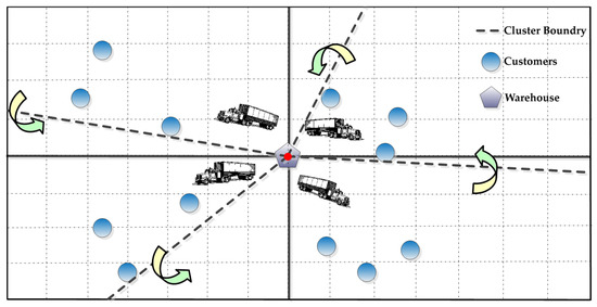
Figure 4. An illustration of clustering by the sweep method.

The total cost is accumulated by the fixed cost of vehicles used (operational cost) and transportation costs as vehicles travel from one customer to another. In some cases, the aggregated service time consumed by each customer is also considered. Overall, the shorter the distance traveled by vehicles, the lower the total cost incurred. Figure 5 exemplifies the hierarchies of the proposed two-phase algorithm for 10 customers with homogeneous demand served by 2 vehicles as well as the chromosome encoding format in this study.

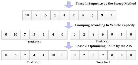
Figure 5. An illustration of 10 nodes with homogeneous demand served by 2 vehicles.

4.2. AIS Procedure

As mentioned previously, the AIS was successfully implemented to solve combinatorial optimization and abnormal detection problems. For data representation, we used chromosomes to denote routing sequences. All suppliers and retailers were assigned a unique number. We made the variation field of each cell, and its dimensions (length of chromosome) equivalent to the suppliers’ (for pickup routes) or customers’ (for delivery routes) numbers to be served, as shown in Figure 5. Therefore, the cells’ chromosomes represent the nodes of the positions to be visited. In the meantime, the suppliers’ or customers’ sequences also mean the routing of orders. First, somatic hypermutation will be selected to make cells evolve, which can search for any feasible cells in the solution field. Next, we calculate the affinities between the antigen-antibodies and antibodies-antibodies according to the objective function. After iterations, the relationship between antigens and antibodies has a greater affinity. Moreover, elimination is a mechanism that will delete worse cells with each iteration. With affinity maturation and elimination, the cells will mutate toward the better-quality field of solution. In this case, each iteration individually will preserve the best cell, which means a higher affinity value.

In the proposed sAIS optimization algorithm, the principles of each antibody mutation have four parts. The basic components of the sAIS applied in the VRPCD are shown as follows:

• Antigen: the antigen mimics the equations of the VRPCD model, which represent the formulas for the objection function and constraint functions;
• Antibody: The antibody is the candidate solution for the VRPCD model. The strings of solutions refer to the visiting sequence of suppliers or customers. The antibodies are feasible sets of models for the problem;
• Cell: the cell represents the ID of suppliers or customers;
• Population size: the number of antibodies (feasible solutions of the VRPCD model) that are used per iteration;
• Number of clones for each cell: number of times antibodies are reproduced per iteration;
• Stopping criterion: the sAIS optimization procedure will not be terminated until the maximum number of iterations is reached.

The proposed sAIS optimization approach has a mechanism with the inside operation processes:

• Somatic Recombination

Somatic recombination is one of the gene rearrangement processes that involves cutting out small regions of DNA and then putting the remaining pieces of DNA back together in an error-prone way in the adaptive immune system. For every iteration of our proposed algorithm, we randomly create a new set of antibodies by using the somatic recombination process in order to search for optimized solutions;

2.

Somatic Hypermutation

There are five types of immune mutations that we use in our proposed sAIS algorithm. Each type has a different function. If the cost of objection function of antibodies in IgM is larger than the cost of the old ones, we randomly selected one of four kinds of immune mutations to operate in the next step of mutation in the same iteration. In addition to the traditional four types of immune mutations, we proposed a new immune mutation, called IgG₂, to further improve the performance of the sAIS optimizations:

• • IgM mode: In the vehicle’s route of sequence s, randomly select two suppliers or customers, i and j. Inverse the sequence of suppliers or customers between i and j as shown in Figure 6. It is noted that if |i − j| < 2 it is not allowed to be mutated;
    

    Figure 6. The operation of IgM mode.
  • IgG mode: In the vehicle’s route of sequence s, randomly select two suppliers or customers, i and j. Swap these two suppliers or customers in the neighbor of s;
  • IgA mode: In the vehicle’s route of sequence s, randomly select two suppliers or customers, i and j. Insert the suppliers or customers i to the sequence’s jth position in the neighbor of s as shown in Figure 7;
    

    Figure 7. The operation of IgA mode.
  • IgG₂ mode: In the vehicle’s route of sequence s, let i₁, i₂, j₁, and j₂ be randomly selected as four suppliers or customers in the sequence. Swap i₁ to j₁ and i₂ to j₂ in the neighbor of s as shown in Figure 8;
    

    Figure 8. The operation of IgG₂ mode.
  • IgE mode: Both the IgG mode and the IgA mode are applied in this mutation. In the vehicle’s route of sequence s, randomly select two suppliers or customers, i and j. A new sequence s’ is provided by swapping i and j. Then, in the sequence s’ randomly selected i’ and j’ will be suppliers and customers, respectively, and have a position in the sequence. Inserting the suppliers or customers i to the sequence position j in the neighbor of s’;

3.

Affinity Maturation

Affinity means the total cost of the vehicles routed from the objection function of the VRPCD model. Some mutant antibodies with lower costs may be generated after several iterations of somatic hypermutation. Then, from iteration to iteration, the cost of producing antibodies will steadily decrease. This phenomenon is called affinity maturation;

4.

Elimination Process

The antibodies will be stored in a limited list per iteration. Except for the best antibody, the antibodies that were produced and mutated per iteration were deleted from previous iterations. As a result, antibodies will search for alternative solution spaces for the VRPCD;

5.

Escape Criterion

We designed an escape criterion for searching the antibody in the global optimization to prevent the search from entering the same solution space and remaining in the local optimum.

Figure 9 and Algorithm 1 show the proposed procedure of the sAIS algorithm.

Algorithm 1: The proposed sAIS algorithm.

Initialization: Create a population of p antibodies randomly (p is the size of the antibody population) For each iteration do: For each antibody do:            Somatic recombination            Calculate affinity of the antibody            Somatic hypermutation:                       IgM                       Decode the new string                       If the objective function (new) < the objective function (old):                                  antibody = new string;                       else:                                  Choose IgG, IgE, IgA or IgG2                                  Decode the new string                                  If the objective function (new) < the objective function (old):                                             antibody = new string                                  else:                                             antibody = antibody            Eliminate antibodies except the best antibody in the population            Reserve the best antibody in the population to affect velocity            If the objective function (new) = the objective function (old):                       Count++            If count attain list length:                       Generate the new antibodies randomly   End For Loop   If stopping criteria = false:            Continue   else:            Break End For Loop

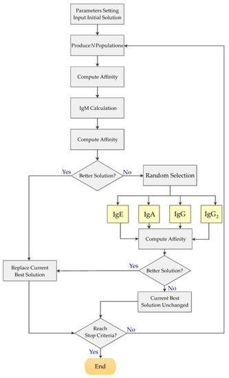
Figure 9. The processes of the proposed sAIS flowchart.

5. Computational Experiments

First, a preliminary investigation of the optimal parameter settings for the proposed algorithm is presented here. Next, 60 VRPPD benchmark problems were retrieved from the VRP Web (http://www.bernabe.dorronsoro.es/vrp/ accessed on 3 February 2023) as the criteria to evaluate the performance of the proposed heuristics. The comparison set is based on the GA algorithm, which is functioned by the customized software Palisade Evolver (https://www.palisade.com/evolver/) industrial edition 5.5.1, the Genetic Algorithm Solver plug-in for Microsoft Excel 2016.

5.1. Preliminary Tests

In the preliminary experiment, the design of experiments (DOE) was conducted to decide the optimal parameter settings for the sAIS optimization. The size of the population and escape list were acquired through the experimentation methodology. One randomly selected instance from the 60 testing problems was used to execute the experiment methodology. The parameter of population size, after an initial trial-and-error process, was located in the interval of [100, 500], and we used the set of {100, 200, 300, 400, and 500} to run the single factor factorial design experiment at 5 levels. Figure 10 shows the mean plot of the population size factor from the results of the experiments. The variable y is the objective function’s minimized value (fitness value), as is the y-axis in Figure 10 and Figure 11.

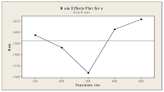
Figure 10. The mean plot of population size for a one-factor factorial design.

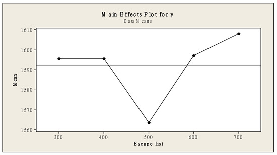
Figure 11. The mean plot of the escape list for a one-factor factorial design.

When the length of the escape list is attained, the AIS algorithm will jump out of the present field. The DOE also determined the length from large numbers in the interval [300, 700], and we chose {300, 400, 500, 600, and 700} as the 5 levels for the single factor factorial design experiment. Figure 8 shows the mean plot of the escape list factor from the results of the experiment.

It is found that the sAIS method can generate a better-quality solution when the population size and escape list factors are assigned to 300 and 500. According to the literature review, the maximum iteration was set at 100,000 trials as the termination criterion in our experiments. These settings were used in the following experiment for the sAIS algorithm. On the other hand, the population size of genes in the GA method was set at 50; the mutation rate is 0.06; and the crossover rate is 0.15. The maximum iteration number was 5000 trials with 30 replications for each instance.

5.2. Experiment Results

A total of 60 benchmark datasets with homogeneous demands were used in our experiment. Each instance is replicated for 30 runs for both the sAIS algorithm and the GA method. The solution from the sweep method, which generates proper clusters for shipment grouping of vehicles, is then picked up as the initial solution for both the sAIS and the GA methods. The comparison of performance between the two methods is computed based on the average improvement rate (AIR), as shown in Equation (14). The experimentation results are given in Table 1.

$$\mathrm{Average} \mathrm{Improvement} \mathrm{Rate} (\mathrm{AIR})=\frac{|{\mathrm{AIS}}_{\mathrm{Average} \mathrm{Cos}\mathrm{t}}-{\mathrm{GA}}_{\mathrm{Average} \mathrm{Cos}\mathrm{t}|}}{{\mathrm{GA}}_{\mathrm{Average} \mathrm{Cos}\mathrm{t}}} \times 100\%.$$

(14)

Table 1. Performance comparisons between sAIS and GA.

No. Instances	GA		sAIS		AIR
	Average Cost	Average Time (s)	Average Cost	Average Time (s)
1P1	1683.22	604.5	1563.57	120.64	7.11%
2P1	1831.25	624	1671.51	111.38	8.72%
3P1	2075.44	624	1971.64	108.68	5.00%
4P1	1446.27	604.5	1439.02	126.73	0.50%
5P1	1515.79	624	1508.69	116.22	0.47%
6P1	1895.14	624	1819.36	112.09	4.00%
7P1	1790.83	643.5	1580.49	123.12	11.75%
8P1	1826.89	624	1659.31	104.11	9.17%
9P1	2429.49	624	1651.10	111.32	32.04%
10P1	1735.36	624	1488.57	103.91	14.22%
11P1	1859.02	643.5	1651.24	136.64	11.18%
12P1	2244.29	624	2031.68	136.61	9.47%
13P1	1604.56	624	1538.53	138.81	4.12%
14P1	1853.96	643.5	1680.49	140.23	9.36%
15P1	2091.15	663	1971.21	131.98	5.74%
16P1	1393.43	702	1363.70	170.57	2.13%
17P1	1487.11	663	1457.43	143.20	2.00%
18P1	1972.85	624	1799.52	137.73	8.79%
19P1	1120.58	624	1076.95	179.50	3.89%
20P1	1181.41	643.5	1170.37	164.43	0.93%
21P1	1641.65	624	1519.44	135.39	7.44%
22P1	1243.36	624	1132.10	176.54	8.95%
23P1	1246.59	663	1221.70	157.51	2.00%
24P1	1685.82	663	1550.75	137.61	8.01%
25P1	1035.99	643.5	1021.97	172.06	1.35%
26P1	1132.80	663	1116.50	170.57	1.44%
27P1	1721.06	643.5	1460.14	137.45	15.16%
28P1	1242.39	624	1202.44	183.15	3.22%
29P1	1338.65	663	1284.38	163.36	4.05%
30P1	1747.52	643.5	1616.69	138.48	7.49%
31P1	991.99	663	960.42	112.47	3.18%
32P1	1291.67	663	1202.92	113.12	6.87%
33P1	1721.57	663	1626.53	100.73	5.52%
34P1	971.77	663	956.98	117.75	1.52%
35P1	1180.81	624	1140.58	101.94	3.41%
36P1	1746.42	624	1554.76	101.45	10.97%
37P1	1070.18	604.5	944.67	109.23	11.73%
38P1	1274.88	624	1143.66	119.46	10.29%
39P1	1767.73	624	1553.02	115.70	12.15%
40P1	1090.22	643.5	1001.72	123.07	8.12%
41P1	1276.28	624	1212.92	101.59	4.96%
42P1	1679.75	624	1640.76	121.74	2.32%
43P1	1153.37	624	975.59	123.60	15.41%
44P1	1356.32	643.5	1166.58	111.69	13.99%
45P1	1723.25	624	1573.59	104.94	8.68%
46P1	1195.50	624	1083.37	103.39	9.38%
47P1	1373.71	643.5	1233.93	100.70	10.18%
48P1	1697.67	663	1618.59	114.34	4.66%
49P1	1286.97	702	1264.74	113.89	1.73%
50P1	1278.76	663	1264.71	101.67	1.10%
51P1	1741.72	643.5	1662.47	140.89	4.55%
52P1	1314.23	663	1154.11	138.25	12.18%
53P1	1451.27	624	1305.02	132.65	10.08%
54P1	1952.70	624	1742.00	124.55	10.79%
55P1	1308.87	624	1192.67	137.26	8.88%
56P1	1418.42	643.5	1333.62	136.96	5.98%
57P1	1888.41	624	1792.38	132.35	5.09%
58P1	1344.08	624	1153.09	139.39	14.21%
59P1	1371.34	663	1311.74	140.85	4.35%
60P1	1822.68	663	1760.34	136.58	3.42%
Avg. AIR		639.275		129.37	7.26%
Std. of AIR					0.0521
Max. AIR					32.04%
Min. AIR					0.47%

As listed, the 60 benchmark problems were sorted into 20 subgroups with three instances in each, based on the node coordinates assigned. Instances within one group are given identical node coordinates, except for the position where the cross-docking facility is located. Each set of the 60 instances contains 100 nodes, comprising both pickup and delivery customers. Each node is associated with a known demand of 10 units, while each vehicle dispatched is constrained by a capacity limit of 100 units. Examples of optimized routing sequences are shown in the Appendix A.

The computational results showed that the solution quality of the sAIS method is superior to the GA, outperforming each with an average improvement rate and lowest improvement rate of 11.98% and 9.47%, respectively, on the basis of average solution quality. In addition, the sAIS optimization, which has the lowest cost, was able to discover new, better solutions than the GA did in all 60 benchmarks, even though the computation time of the sAIS algorithm method takes longer; however, it is still a reasonable amount of time. Moreover, the maximum rate of improvement on average solution quality is 30.03%, whereas the minimum rate is acquired at 1.28%, indicating that the performance of the sAIS method is robust and competitive with the GA method. Nevertheless, all problems’ average improvement rate was better able to discover new solutions than the GA did.

Finally, a one-sided, two-sample t-test was conducted to verify the performance of the two methods. The hypothesis test is:

H₀: μ_GA − μ_sAIS = 0

H_A: μ_GA − μ_sAIS > 0

the results showed that the t-value = 2.09 and the p-value = 0.019. Because the p-value is less than the 0.05 significant level, we reject the null hypothesis and conclude that μ_GA is significantly greater than μ_sAIS. That is, the total cost, including transportation costs and operational costs, generated by the sAIS approach is smaller than the total cost generated by the GA in our experiments.

6. Conclusions and Future Research

In this research, a novel sAIS algorithm is proposed to approach the combinatorial optimal solution of the VRPCD. The primary objectives of this work include the integration of the operation of cross-docking and the optimal vehicle routing schedule into the design of supply chain optimization. A significant development lies in the synchronization between upstream suppliers and downstream retailers, where both sides of the supply chain are simultaneously considered to collaborate on the physical flow of goods in each inbound and outbound process. Manufacturers can reduce logistics costs by building IoT monitoring technology into smart logistics IT systems to track its location in real-time, reduce inventory levels in warehouses, monitor environmental conditions, and optimize the routing sequence for trucks for smart city infrastructure.

The computational results show that the sAIS model is effective for solving the VRPCD. The effectiveness of the method comes from the two-phase mechanism. In the initial route generation phase, the initial solution was generated by the sweep method before being input into the route’s optimization phase with the AIS algorithm. The combination of the two-phase approach ensures that the sAIS method yields quality solutions.

A total of 60 benchmark problems were deployed to investigate the applicability of the proposed sAIS method. The experimental results showed that the sAIS method was able to produce significant improvements over the GA, surpassing each testing problem. Additionally, the sAIS method was able to discover better solutions than the GA method for all 60 benchmark problems, and the sAIS’s search time is faster than the GA. It found sAIS to be a useful methodology. As artificial intelligence research rapidly increases, more simulations from human body systems could be used to improve the solution quality of the AIS optimization, and the AIS optimization could be applied to other research problems in the operations research field, such as multiple-criteria decision-making problems or supplier selection problems, etc.

References

- Khanh, Q.V.; Hoai, N.V.; Manh, L.D.; Le, A.N.; Jeon, G. Wireless communication technologies for IoT in 5G: Vision, applications, and challenges. Wirel. Commun. Mob. Comput. 2022, 2022, 3229294. [Google Scholar] [CrossRef]
- Kamruzzaman, M.M. Key technologies, applications and trends of Internet of Things for energy-efficient 6G wireless communication in smart cities. Energies 2022, 15, 5608. [Google Scholar] [CrossRef]
- Qadir, Z.; Le, K.N.; Saeed, N.; Munawar, H.S. Towards 6G Internet of Things: Recent advances, use cases, and open challenges. ICT Express 2022, In press. [Google Scholar] [CrossRef]
- Kulwiec, R. Crossdocking as a supply chain strategy. Association for Manufacturing Excellence. 2004. Available online: https://www.ame.org/sites/default/files/target_articles/04-20-3-Crossdocking.pdf (accessed on 23 January 2023).
- Stępień, M.; Łęgowik-Świącik, S.; Skibińska, W.; Turek, I. Identification and measurement of logistics cost parameters in the company. Transp. Res. Procedia 2016, 16, 490–497. [Google Scholar] [CrossRef]
- Laporte, G. Fifty years of vehicle routing. Transp. Sci. 2009, 43, 408–416. [Google Scholar] [CrossRef]
- He, M.; Shen, J.; Wu, X.; Luo, J. Logistics space: A literature review from the sustainability perspective. Sustainability 2018, 10, 2815. [Google Scholar] [CrossRef]
- Astachova, I.F.; Zolotukhin, A.E.; Kurklinskaya, E.Y.; Belyaeva, N.V. The application of artificial immune system to solve recognition problems. J. Phys. Conf. Ser. 2019, 1203, 012036. [Google Scholar] [CrossRef]
- Wang, D.; Liang, Y.; Dong, H.; Tan, C.; Xiao, Z.; Liu, S. Innate immune memory and its application to artificial immune systems. J. Supercomput. 2022, 78, 11680–11701. [Google Scholar] [CrossRef]
- Silva, G.C.; Dasgupta, D. A survey of recent works in artificial immune systems. In Handbook on Computational Intelligence; Angelov, P.P., Ed.; World Scientific Publishing Co Pte Ltd.: Singapore, 2016; pp. 547–586. [Google Scholar] [CrossRef]
- Park, H.; Choi, J.E.; Kim, D.; Hong, S.J. Artificial immune system for fault detection and classification of semiconductor equipment. Electronics 2021, 10, 944. [Google Scholar] [CrossRef]
- Miralvand, M.; Rasoolzadeh, S.; Majidi, M. Proposing a features preprocessing method based on artificial immune and minimum classification errors methods. J. Appl. Res. Technol. 2015, 13, 106–112. [Google Scholar] [CrossRef]
- Ma, J.; Gao, L.; Shi, G. An Improved Immune Clonal Selection Algorithm and Its Applications for VRP. In Proceedings of the 2009 IEEE International Conference on Automation and Logistics, Shenyang, China, 5–7 August 2009. [Google Scholar] [CrossRef]
- Arabani, A.R.B.; Ghomi, S.M.T.F.; Zandieh, M. Meta-heuristics implementation for scheduling of trucks in a cross-docking system with temporary storage. Expert Syst. Appl. 2011, 38, 1964–1979. [Google Scholar] [CrossRef]
- Arabani, A.R.B.; Zandieh, M.; Ghomi, S.M.T.F. Multi-objective genetic-based algorithms for a cross-docking scheduling problem. Appl. Soft Comput. 2011, 11, 4954–4970. [Google Scholar] [CrossRef]
- Arabani, A.R.B.; Zandieh, M.; Ghomi, S.M.T.F. A cross-docking scheduling problem with sub-population multi-objective algorithms. Int. J. Adv. Manuf. Technol. 2012, 58, 741–761. [Google Scholar] [CrossRef]
- Lee, Y.H.; Jung, J.W.; Lee, K.M. Vehicle routing scheduling for cross-docking in the supply chain. Comput. Ind. Eng. 2006, 51, 247–256. [Google Scholar] [CrossRef]
- Gunawan, A.; Widjaja, A.T.; Vansteenwegen, P.; Yu, V.F. A matheuristic algorithm for the vehicle routing problem with cross-docking. Appl. Soft Comput. 2021, 103, 107163. [Google Scholar] [CrossRef]
- Dantzig, G.B.; Ramser, J.H. The truck dispatching problem. Manage. Sci. 1959, 6, 80–91. [Google Scholar] [CrossRef]
- Vidal, T.; Crainic, T.G.; Gendreau, M.; Prins, C. Heuristics for multi-attribute vehicle routing problems: A survey and synthesis. Eur. J. Oper. Res. 2013, 231, 1–21. [Google Scholar] [CrossRef]
- Hertrich, C.; Hungerländer, P.; Truden, C. Sweep algorithms for the capacitated vehicle routing problem with structured time windows. In Operations Research Proceedings 2018; Springer: Cham, Switzerland, 2019; pp. 127–133. [Google Scholar] [CrossRef]
- Agárdi, A.; Kovács, L.; Bányai, T. Ontology support for vehicle routing problem. Appl. Sci. 2022, 12, 12299. [Google Scholar] [CrossRef]
- Kamruzzaman, M.M. Hybrid modified ant system with sweep algorithm and path relinking for the capacitated vehicle routing problem. Heliyon 2021, 7, e08029. [Google Scholar] [CrossRef]
- Borčinová, Z. Kernel search for the capacitated vehicle routing problem. Appl. Sci. 2022, 12, 11421. [Google Scholar] [CrossRef]
- Laporte, G.; Nobert, Y.; Desrochers, M. Optimal routing under capacity and distance restrictions. Oper. Res. 1984, 43, 1050–1073. [Google Scholar] [CrossRef]
- Mosheiov, G. Vehicle routing with pick-up and delivery: Tour partitioning heuristics. Comput. Ind. Eng. 1998, 34, 669–684. [Google Scholar] [CrossRef]
- Baker, B.M.; Ayechew, M.A. A genetic algorithm for the vehicle routing problem. Comput. Oper. Res. 2003, 30, 787–800. [Google Scholar] [CrossRef]
- Osman, I.H. Metastrategy simulated annealing and tabu search algorithms for the vehicle routing problem. Ann. Oper. Res. 1993, 41, 421–451. [Google Scholar] [CrossRef]
- Taillard, É. Parallel iterative search methods for vehicle routing problems. Networks 1993, 23, 661–673. [Google Scholar] [CrossRef]
- Gendreau, M.; Hertz, A.; Laporte, G. A Tabu search heuristic for the vehicle routing problem. Manage. Sci. 1994, 40, 1276–1290. [Google Scholar] [CrossRef]
- Taillard, É.; Badeau, P.; Gendreau, M.; Guertin, F.; Potvin, J.-Y. A tabu search heuristic for the vehicle routing problem with soft time windows. Transp. Sci. 1997, 31, 101–195. [Google Scholar] [CrossRef]
- Bell, J.E.; McMullen, P.R. Ant colony optimization techniques for the vehicle routing problem. Adv. Eng. Inform. 2004, 18, 41–48. [Google Scholar] [CrossRef]
- Wu, H.; Gao, Y.; Wang, W.; Zhang, Z. A hybrid ant colony algorithm based on multiple strategies for the vehicle routing problem with time windows. Complex Intell. Syst. 2021, 1–18. [Google Scholar] [CrossRef]
- Ky Phuc, P.N.; Phuong Thao, N.L. Ant colony optimization for multiple pickup and multiple delivery vehicle routing problem with time window and heterogeneous fleets. Logistics 2021, 5, 28. [Google Scholar] [CrossRef]
- Lo, S.-C. A particle swarm optimization approach to solve the vehicle routing problem with cross-docking and carbon emissions reduction in logistics management. Logistics 2022, 6, 62. [Google Scholar] [CrossRef]
- Lo, S.-C.; Shih, Y.-C. A genetic algorithm with quantum random number generator for solving the pollution-routing problem in sustainable logistics management. Sustainability 2021, 13, 8381. [Google Scholar] [CrossRef]
- Jerne, N.K. Towards a network theory of the immune system. Ann. Immunol. 1974, 125C, 373–389. [Google Scholar]
- Farmer, J.D.; Packard, N.H.; Perelson, A.S. The immune system, adaption, and machine learning. Physica. D. 1986, 22, 187–204. [Google Scholar] [CrossRef]
- Kephart, J.O. A biologically inspired immune system for computers. In Artificial Life IV: The Fourth International Workshop on the Synthesis and Simulation of Living Systems; Brooks, R.A., Maes, P., Eds.; The MIT Press: Cambridge, MA, USA, 1994; pp. 130–139. [Google Scholar] [CrossRef]
- Hunt, J.; Timmis, J.; Cooke, E.; Neal, M.; King, C. Jisys: The envelopment of an artificial immune system for real world applications. In Artificial Immune Systems and Their Applications; Dasgupta, D., Ed.; Springer: Berlin/Heidelberg, Germany, 1999; pp. 157–186. [Google Scholar] [CrossRef]
- Mrowczynska, B.; Ciesla, M.; Krol, A.; Sladkowski, A. Application of artificial intelligence in prediction of road freight transportation. Promet—TrafficTransp. 2017, 29, 363–370. [Google Scholar] [CrossRef]
- Mabrouk, E.; Raslan, Y.; Hedar, A.-R. Immune system programming: A machine learning approach based on artificial immune systems enhanced by local search. Electronics 2022, 11, 982. [Google Scholar] [CrossRef]
- Cutello, V.; Nicosia, G. An immunological approach to combinatorial optimization problems. In Advances in Artificial Intelligence—IBERAMIA 2002; Garijo, F.J., Riquelme, J.C., Toro, M., Eds.; Lecture Notes in Computer Science book series; Springer: Berlin/Heidelberg, Germany, 2002; Volume 2527, pp. 361–370. [Google Scholar] [CrossRef]
- Parham, P. The Immune System, 4th ed.; Garland Science Publishing: New York, NY, USA, 2014; ISBN 978-08153443667. [Google Scholar]
- Kim, Y.; Lee, H.; Park, K.; Park, S.; Lim, J.-H.; So, M.K.; Woo, H.-M.; Ko, H.; Lee, J.-M.; Lim, S.H.; et al. Selection and characterization of monoclonal antibodies targeting middle east respiratory syndrome coronavirus through a human synthetic fab phage display library panning. Antibodies 2019, 8, 42. [Google Scholar] [CrossRef]
- Yadav, D.; Agarwal, S.; Pancham, P.; Jindal, D.; Agarwal, V.; Dubey, P.K.; Jha, S.K.; Mani, S.; Dey, A.; Jha, N.K.; et al. Probing the immune system dynamics of the COVID-19 disease for vaccine designing and drug repurposing using bioinformatics tools. Immuno 2022, 2, 344–371. [Google Scholar] [CrossRef]
- Engin, O.; Döyen, A. A new approach to solve hybrid flow shop scheduling problems by artificial immune system. Future Gener. Comput. Syst. 2004, 20, 1083–1095. [Google Scholar] [CrossRef]
- Chung, T.-P.; Liao, C.-J. An immunoglobulin-based artificial immune system for solving the hybrid flow shop problem. Appl. Soft Comput. 2013, 13, 3729–3736. [Google Scholar] [CrossRef]
- Pan, S.; Manabe, N.; Yamaguchi, Y. 3D structures of IgA, IgM, and components. Int. J. Mol. Sci. 2021, 22, 12776. [Google Scholar] [CrossRef] [PubMed]
- de Sousa-Pereira, P.; Woof, J.M. IgA: Structure, function, and developability. Antibodies 2019, 8, 57. [Google Scholar] [CrossRef] [PubMed]
Disclaimer/Publisher’s Note: The statements, opinions and data contained in all publications are solely those of the individual author(s) and contributor(s) and not of MDPI and/or the editor(s). MDPI and/or the editor(s) disclaim responsibility for any injury to people or property resulting from any ideas, methods, instructions or products referred to in the content. |
© 2023 by the authors. Licensee MDPI, Basel, Switzerland. This article is an open access article distributed under the terms and conditions of the Creative Commons Attribution (CC BY) license (https://creativecommons.org/licenses/by/4.0/).