Investigation of the Effect of the Voltage Drop and Cable Length on the Success of Starting the Line-Start Permanent Magnet Motor in the Drive of a Centrifugal Pump Unit

Abstract

The use of Line-Start Permanent Magnet Synchronous Motors (LSPMSM) improves the efficiency of conventional direct-on-line electric motor-driven fluid machinery such as pumps and fans. Such motors have increased efficiency compared to induction motors and do not have an excitation winding compared to classical synchronous motors with an excitation winding. However, LSPMSMs have difficulty in starting mechanisms with a high moment of inertia. This problem can be exacerbated by a reduced supply network voltage and a voltage drop on the cable. This article investigates the transients during the startup of an industrial centrifugal pump with a line-start permanent magnet synchronous motor. The simulation results showed that when the voltage on the motor terminals is reduced by 10%, the synchronization is delayed. The use of the cable also leads to a reduction in the voltage at the motor terminals in a steady state, but the time synchronization delay is more significant than that with a corresponding reduction in the supply voltage. The considered simulation example shows that the line-start permanent magnet synchronous motor has no problems with starting the pumping unit, even with a reduced supply voltage. The conclusions of this paper support a wider use of energy-efficient electric motors and can be used when selecting an electric motor to drive a centrifugal pump.

1. Introduction

At present, most typical industrial mechanisms (pumps, fans, blowers, compressors, etc.) of medium and small power with a direct start from the mains are driven by induction motors (IMs) [1,2,3,4]. IMs are reliable and affordable [5], but their significant drawback is their relatively low efficiency. For this reason, they usually have a relatively low energy efficiency class, not exceeding IE3, in accordance with the IEC 60034-30-2 standard “Rotating electric machines—Part 30-2: efficiency class of variable speed AC motors (IE code)” [6]. Rising prices for electricity [7], the tightening of the requirements of the European regulator for the energy efficiency of electric motors used in enterprises [8] and requirements to reduce CO₂ consumption [9] force enterprises to use more efficient motors. However, improving the efficiency of induction motors leads to a significant increase in the cost and dimensions of the machine [1].

Linear start permanent magnet motors (LSPMSMs) can be a more energy-efficient alternative in direct-on-line start applications compared to induction motors. LSPMSMs have a stator design similar to IMs, a squirrel cage and permanent magnets on the rotor. LSPMSMs are already commercially available as general-purpose motors [10,11,12] and as part of a compressor drive [13]. Due to their principle of operation, such motors can have an IE4 energy efficiency class and higher, without going beyond the dimensions of induction motors with the IE3 efficiency class [14] and a constant operating speed, which may be necessary in some applications, such as weaving machines. The use of such motors is limited by their high cost and the technological dependence of their manufacture on the availability of rare earth magnets (China is the main supplier of rare earth magnets).

In addition to this, the LSPMSM has limits on the moment of inertia of the loading mechanism. This is due to the fact that, when starting, the motor works in an asynchronous mode. In this case, the positive torque is characterized as the asynchronous torque of the short-circuited winding, and the magnets create an oscillating torque. If the moment of inertia is large enough, the speed fluctuations are flattened, and, like an induction motor, the LSPMSM does not reach synchronous speed and has a slip at the steady state.

As the inertia decreases, the fluctuations of the speed caused by the fluctuations of the torque increase. The synchronization process is observed when the speed fluctuations are sufficient to achieve synchronous speed. As a rule, in this case, the speed exceeds the synchronous speed, after which calming down follows, i.e., the speed stabilizes and becomes equal to the synchronous speed. The critical moment of inertia of the loading mechanism (the value of the maximum moment of inertia of the loading mechanism with which the LSPMSM synchronization is successful) is indicated in the catalogs of commercially produced LSPMSMs [10,11,12]. Figure 1 compares the IM and LSPMSM designs. In addition to the use of more energy-efficient motors, an increase in the efficiency of pump units can be achieved through the use of frequency converters [15,16], but such an improvement in efficiency requires a significant increase in capital costs.

In energy-saving drives, it is also possible to use a converter-fed PMSM without starting winding [17]. However, the use of a frequency converter leads to a significant increase in the cost of the drive. This increase is especially significant for low-power general-purpose drives, for which the cost of the converter can be several times higher than the cost of the motor.

The starting processes of LSPMSM in the drives of a piston pump [18] and a centrifugal fan [19] were studied. In [18], simulation in Matlab Simulink is given, based on the results from which the data of the torque and current of the LSPMSM were obtained during the start-up and operation in a steady state. In [19], dynamic processes in LSPMSM under fan load were studied. It was found that the start of the fan with a direct start from the network can be implemented by regulating the air flow by throttling. However, there is a lack of research into the process of starting LSPMSM as part of a centrifugal pump. Compared to centrifugal fans, in which the working fluid is a gas, in pumping systems, it is a liquid. A distinctive feature of the liquid is its high density and, hence, a significant kinetic energy accumulated in the pipes.

Typically, the LSPMSM start-up process is investigated at the rated value and frequency of the sinusoidal voltage, without taking into account the voltage drop and the drop in the cable in particular. There are also studies that study the start of LSPMSM [20] and the operation of LSPMSM with distorted voltage [21,22], studies that study the start of IM with reduced voltage [23,24,25] and studies that take into account the effect of the cable [23,24,25]. However, studies on the assessment of the effect of a decrease in the mains voltage and the effect of a cable on the start of an LSPMSM are not presented in the literature.

The starting current of LSPMSMs is five to seven times greater than the rated one, which can cause an additional voltage drop both on the cable and on the internal impedance of the supply transformer. In addition, in the asynchronous mode, the frequency of the electromotive force (EMF) generated by the LSPMSM magnets does not match the frequency of the mains voltage, that is, the action of magnets is equivalent to the action of a closed-circuit generator on the resistance of the winding and the resistance of the network supplying the motor (total impedance of the cable, transformer and other network elements). Thus, magnets not only create an oscillatory torque. Therefore, with an increase in resistance due to the cable, the power of the “generator” and the braking torque increase, which additionally complicates synchronization. As a result, synchronization may not occur, the motor speed will fluctuate at speeds below the synchronous speed and the motor current will pulsate and reach the starting level. Such conditions during prolonged operation lead to the failure of the LSPMSM.

This article, which fills in the gaps noted above in previous studies, is devoted to assessing the success of the synchronization of an LSPMSM as a part of a centrifugal pump unit, taking into account the reduced supply voltage and the influence of the cable. The success of the synchronization is determined using a lumped parameter model, due to the simplicity of the model and the fewer computational efforts required. The parameters for such a model can be determined as a result of the motor’s tests or by calculation, if the details of the motor design are known. To obtain the results of this study, the processes of starting a four-pole LSPMSM in centrifugal pump units of capacities of 0.55 kW and 3 kW are considered. Motors of two power ratings are considered to compare the effect of the cable on the starting process of motors of different powers.

The choice of such a range of rated power of motors for research is due to the fact that, at present, only low-power LSPMSMs are available on the general-purpose motor market [12], which is associated with their increased cost compared to that of IM. Another reason is that, with an increase in the power rating, the available energy efficiency class of mass-produced IMs increases [26]. Additionally, for medium and high powers, it becomes more feasible to use a variable frequency drive.

2. Problem Statement

Figure 2 shows the layout of the pump unit under consideration. The LSPMSM is powered by the three-phase 400 V, 50 Hz voltage via the cable.

The IEC 60038 standard [27] regulates the tolerance to ±10% of the rated phase-to-neutral voltage and additionally allows for a 4% voltage drop due to the connecting cable and ancillary equipment in a steady state. Based on this, the motor start is simulated at a reduced voltage equal to 90% of the rated value. The motor shaft is connected directly to the shaft of a centrifugal pump “Wilo-VeroLine-IPL 65/130” [28], which pumps liquid from one reservoir (tank) to another. The fluid flow enters through a pipe and is regulated by a valve. The model was developed in Matlab Simulink. This scheme is typical for separately operating horizontal pumps.

The following assumptions were made to model the system under consideration:

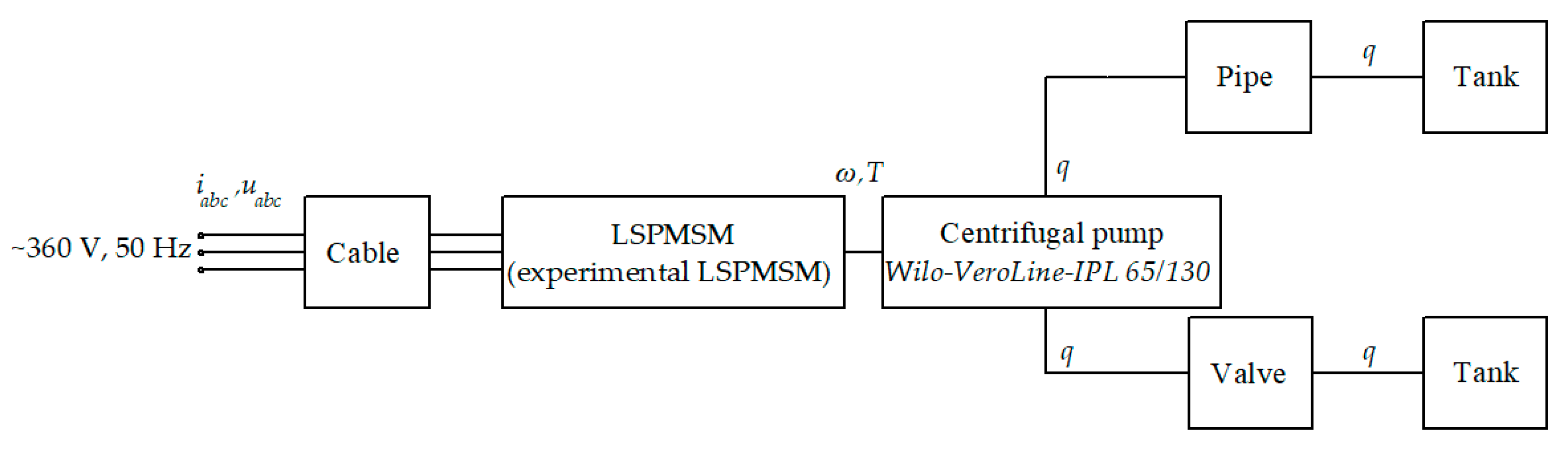
• The fluid is incompressible;
• Only one pump unit operates in the pipeline;
• All hydraulic resistances (such as couplings, filters, etc.), except for the valve resistance, are reduced to one hydraulic diameter and to one pipeline;
• There are no leaks in the hydraulic system.

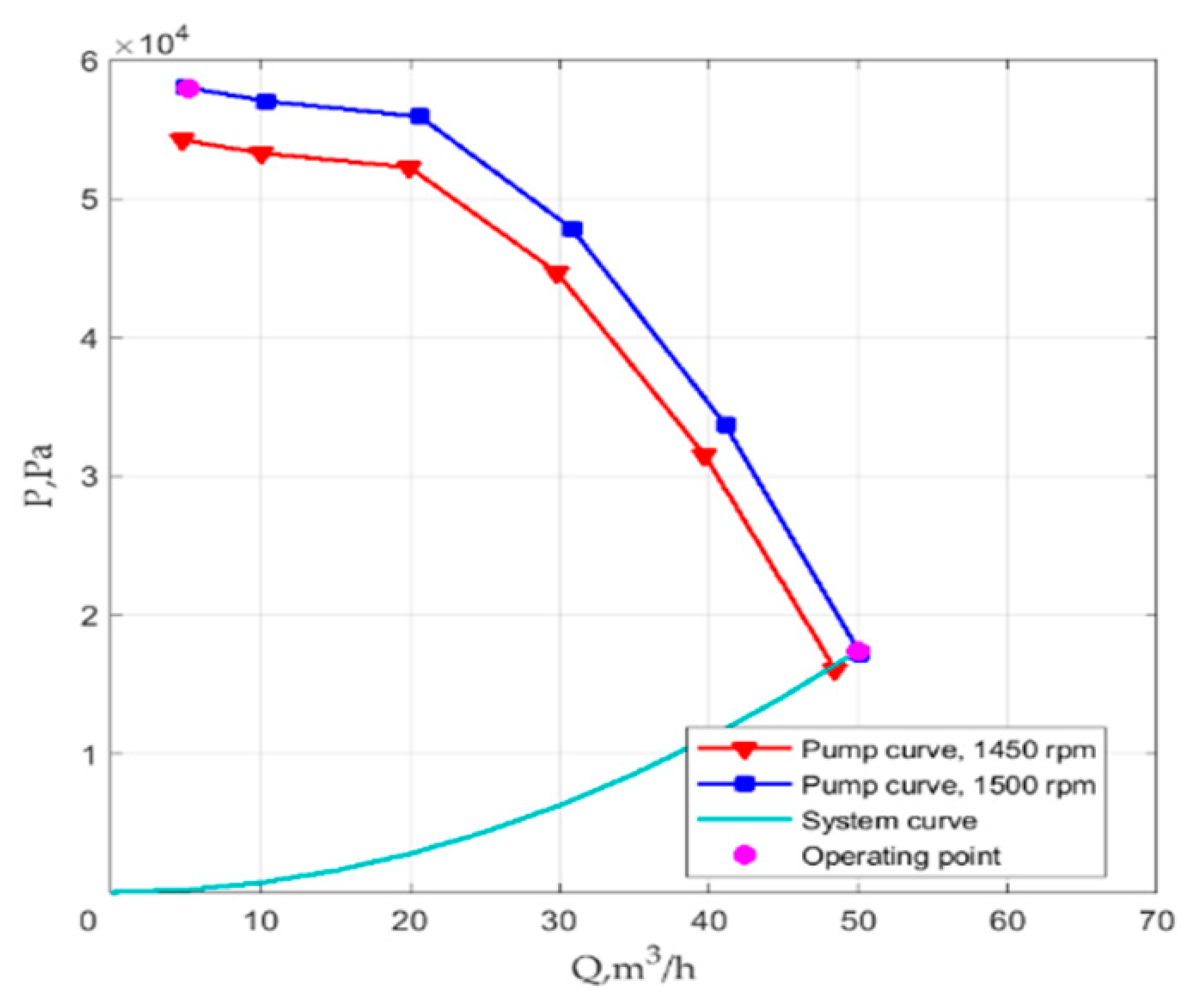
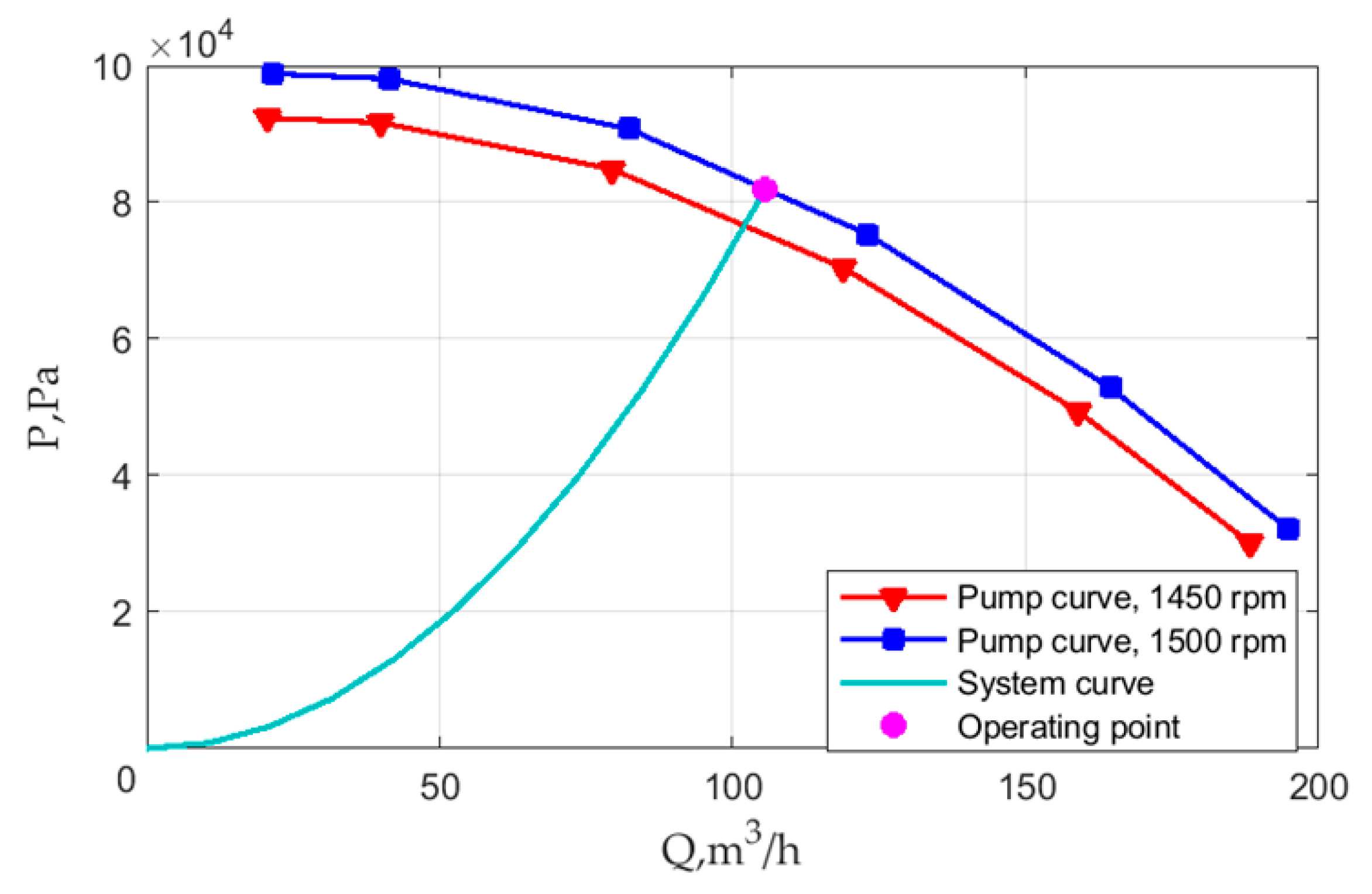
3. Hydraulic System Model

Similarity laws are used to calculate the pressure drop at different angular speeds. The volume flow is calculated using the following formula [29]:

q = q_ref∙(ω/ω_ref);

(1)

where q_ref is the volume flow rate of the pump at the rated speed according to the catalog data; ω—the angular frequency of the rotation of the pump shaft; ω_ref—the rated angular frequency of the rotation of the pump shaft.

The differential pressure is calculated using the following formula:

p = p_ref·ρ/ρ_ref·(ω/ω_ref)²;

(2)

where p_ref is the differential pressure at the rated speed and the rated density, according to the catalog; ρ is the density of the pumped liquid; ρ_ref is the rated density of the pumped liquid.

The mechanical power consumed by the pump is determined according to the following equation:

N = N_ref· ρ/ρ_ref·(ω/ω_ref)³;

(3)

where N_ref is the mechanical power at the rated speed of the pump. The mechanical torque of the pump is:

T = N/ω.

(4)

The inertia of the fluid results in a pressure drop due to the change in the volume flow rate of the fluid. This pressure drop Δp is determined by the following equation [30]:

Δp = ρ·L/A · dq/dt,

(5)

where L is the length of the pipeline; A is the cross-sectional area of the pipe; t is the time variable. The initial condition for the volume flow rate of the fluid is q = 0.

Regulation by means of a valve allows for changing the characteristics of the hydraulic system by means of changing the degree of the valve opening. This method of regulation allows for reducing the hydraulic power during the motor start-up and makes it possible to adjust the operating point of the system throughout the entire life of the pump unit. However, this control method creates additional hydraulic losses [31].

The simulation in this study is carried out in order to determine the conditions under which the LSPMSM successfully enters into synchronism. For this reason, it is especially important to carefully simulate physical processes, including gas flows, occurring at rotation speeds close to the synchronous one.

At sub-synchronous speeds, the phase shift between the motor current and voltage changes slowly, and the LSPMSM alternates between the motor and generator modes until synchronism is achieved. Therefore, for such an analysis, it is sufficient to use a quasi-static model (quasi-stationary), i.e., a model in which, although the hydrodynamic quantities in the elements of a liquid pipeline are assumed to be non-stationary, the relationships connecting them do not contain time derivatives and do not depend on the previous state.

4. LSPMSM Model

When modeling the LSPMSM, it is assumed that:

• The magnetic fields generated by the stator and rotor windings have a sinusoidal spatial distribution;
• The magnetic permeability of the steel is constant;
• The stator and rotor windings are symmetrical;
• Each winding is powered by a separate source;
• The mains voltage phasor is constant throughout the entire starting process, and an increase in the motor current does not cause a decrease in its amplitude;
• Magnetic core losses are not taken into account.

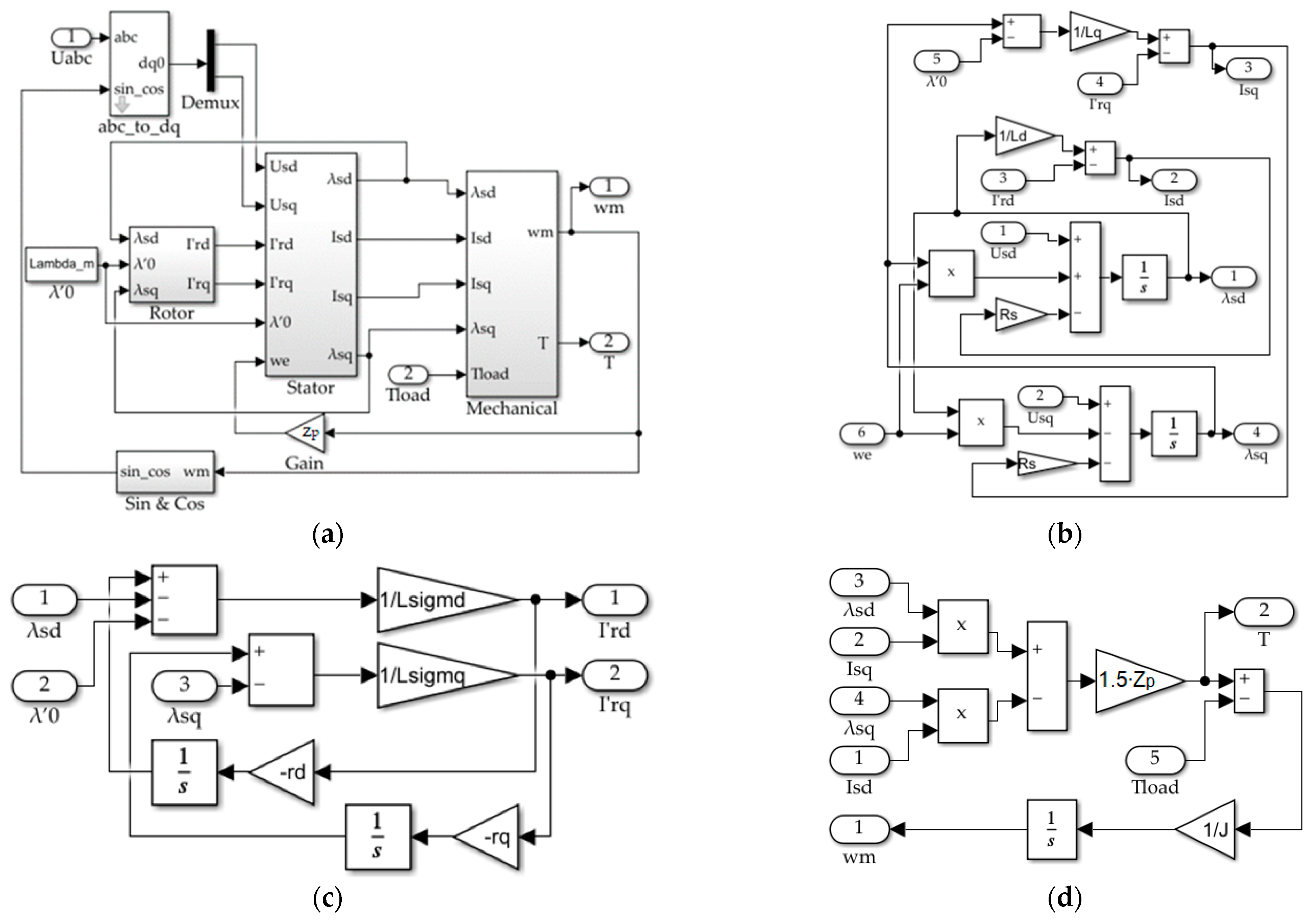
The system of ordinary differential LSPMSM equations to be solved is represented as:

dλ_sd/dt − Z_p · λ_sq · dφ/dt + R_s · I_sd = U_sd;
dλ_sq/dt + Z_p·λ_sd·dφ/dt + R_s · I_sq = U_sq;
dλ’_rd/dt + r’_d · I’_rd = 0;
dλ’_rq/dt + r’_q · I’_rq = 0;
I’_rd = (λ’_rd − λ_sd)/L_σd;
I’_rq = (λ’_rq − [λ_sq − λ’₀])/L_σq;
I_sd = λ_sd/L_sd − I’_rd;
I_sq = (λ_sq − λ’₀)/L_sq − I’_rq;
T = 3/2· Z_p ∙ (λ_sd · I_sq − λ_sq · I_sd);
J ∙ d²φ /dt² = T − T_load.

(6)

where U_sd and U_sq are the stator voltages along the d and q axes; I_sd, I_sq, I’_rd and I’_rq are the stator and rotor currents; L_sd, L_sq, L_rd and L_rq are the stator and rotor total inductances; L_σd and L_σq are the rotor leakage inductances; λ_sd, λ_sq, λ’_rd and λ’_rq are the stator and rotor flux linkages; λ’₀ is the permanent magnet flux linkage; ω_r is the rotor electrical angular frequency; R_s is the stator resistance; Z_p is the number of motor pole pairs; r’_rd and r’_rq are the rotor resistances; φ is the mechanical rotational angle equal to the integral of the motor speed ω; T is the motor torque; T_load is the loading torque; J is the total moment of inertia.

All initial conditions are equal to zero, except for the stator flux along the q-axis λ_sq.0 = λ’₀. Figure 3 shows the implementation of equation system (6) in Simulink.

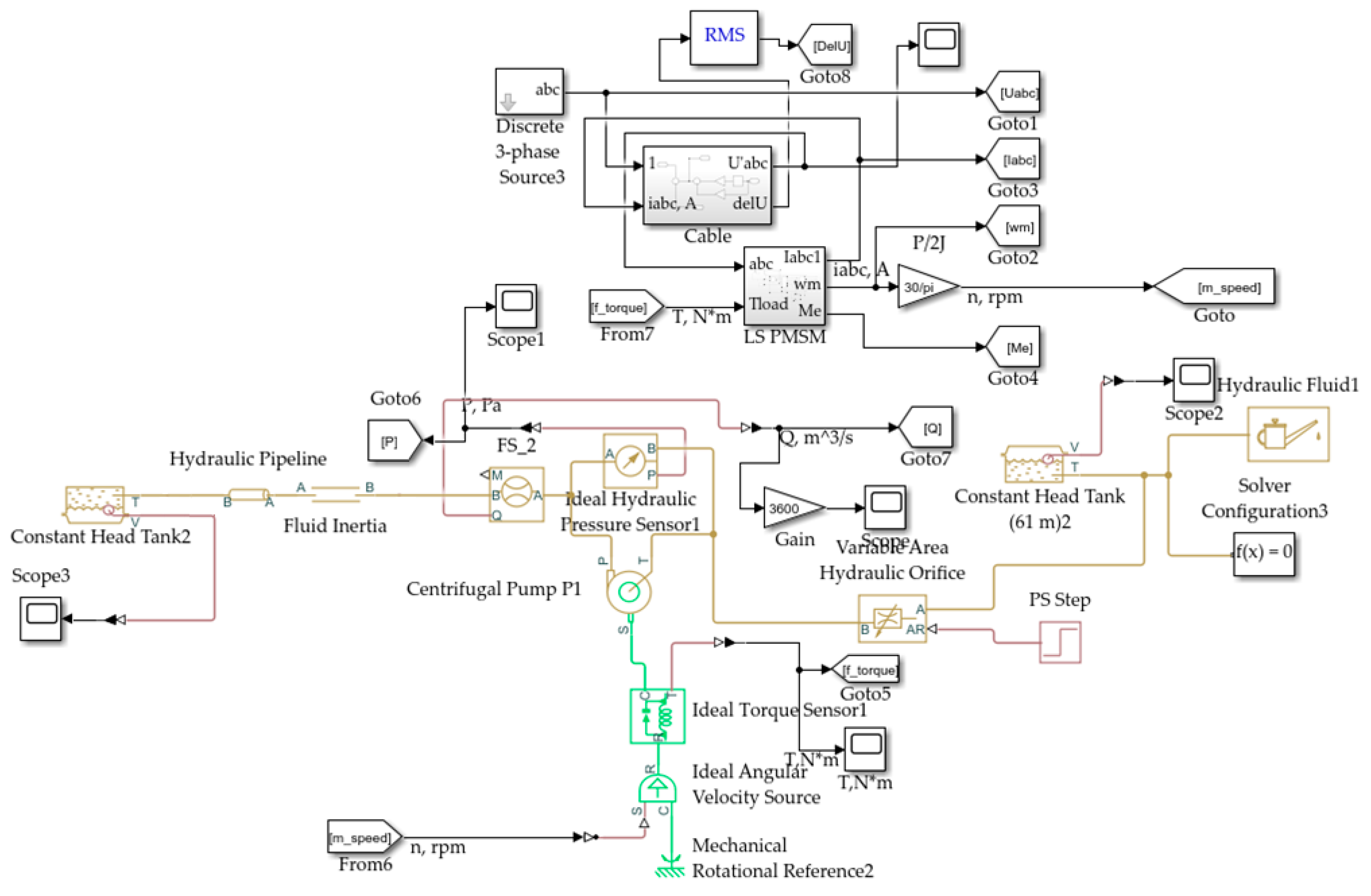
5. Model of the Pump Unit in Matlab Simulink and Parameters of the 0.55 kW Pump Unit

To simulate a pump unit, the Sim-scape/Fluids/Hydraulics library was used in the Matlab Simulink environment, designed to simulate the movement of an ideal fluid. Figure 4 shows a block diagram of the model under study in the Matlab Simulink environment. The model uses the following fluid dynamics modeling blocks: Centrifugal Pump [29], Hydraulic Pipeline [32], Fluid Inertia [30], Variable Area Hydraulic Orifice [33] and Tank [34].

The LSPMSM, fed directly from the mains (“Discrete 3-phase Source”), is mechanically connected directly to the shaft of a centrifugal pump (“Centrifugal Pump”). The pump moves the working fluid from one reservoir to another (“Constant Head Tank” and “Constant Head Tank”) through a pipe (“Hydraulic Pipeline”). The fluid flow is controlled by a valve (“Variable Area Hydraulic Orifice”). Fluid inertia in the pipe is pointed out with a separate element (“Fluid Inertia”). The load torque is measured between the motor shaft and the pump shaft (“Ideal Torque Sensor”) and enters to the input of the motor unit. The motor speed is transmitted to the input (“Ideal Angular Velocity Source”), after which it is connected to the pump shaft. The fluid parameters are set in the block (“Hydraulic Fluid”), and the solver parameters are set in the block (“Solver Configuration”). The parameterization of the model blocks is carried out in such a way that the pump in a steady state operates within the limits of the operating curve given in the catalog. The LSPMSM parameters (rated power 550 W, rated speed 1500 rpm) given in

Table 1. 0.55 kW LSPMSM parameters.

Parameter	Value
Rated power Prate, kW	0.55
Rated line-to-line voltage Urate, V	380
RMS rated stator current, A	1.11
Rated power factor	0.85
Rated frequency f, Hz	50
Pole pair number Zp	2
Stator phase resistance Rs, Ohm	15.3
Total direct inductance Ld, H	0.26
Total quadrature inductance Lq, H	0.15
Leakage direct inductance Lσd, H	0.038
Leakage quadrature inductance Lσq, H	0.051
Rotor direct resistance r’d, Ohm	9.24
Rotor quadrature resistance r’q, Ohm	10.1
Permanent magnet flux linkage λ’0, Wb	0.76
Motor inertia moment Jm, kg·m2	0.003
Pump impeller inertia moment Ji, kg·m2	0.00022

were taken as motor parameters.

The model uses the parameters of a centrifugal pump with a steel impeller “Wilo-VeroLine-IPL 65/130”. The catalog does not specify the moment of inertia, so the moment of inertia of the impeller was assumed to be a tenth of the moment of inertia of the motor, J_i = 0.1·J_m, as proposed for pump drives with an induction motor [35]. Given that the moment of inertia of an M3BP80MA4 induction motor with a rated power of 0.55 kW and a rated speed of 1406 rpm is J_m = 0.0022 kg∙m² [26], the moment of inertia of the pump impeller is:

J_i = 0.1·J_m = 0.1·0.0022 = 0.00022 kg·m².

(7)

Table 2. 0.55 kW pump characteristics.

Flow Q, m3/h	Pressure P, Pa	Braking power Nm, W
4.77	54,229	239.15
10.00	53,304	300.71
19.97	52,259	418.44
29.82	44,691	502.98
39.73	31,490	545.82
48.42	16,106	545.82

shows the catalog characteristics of the pump. These characteristics correspond to a rotational speed of 1450 rpm.

Figure 5 shows the curves of the pump head-flow characteristics corresponding to speeds of 1450 and 1500 rpm, as well as the characteristics of the hydraulic load with the valve open.

For the 0.55 kW pump unit, a pipe with a length of 94.5 m and a cross-sectional area of 0.0137 m² was chosen. The calculation of the characteristics of the pump for rotation speeds other than the rated one is carried out using the laws of similarity (1)–(3).

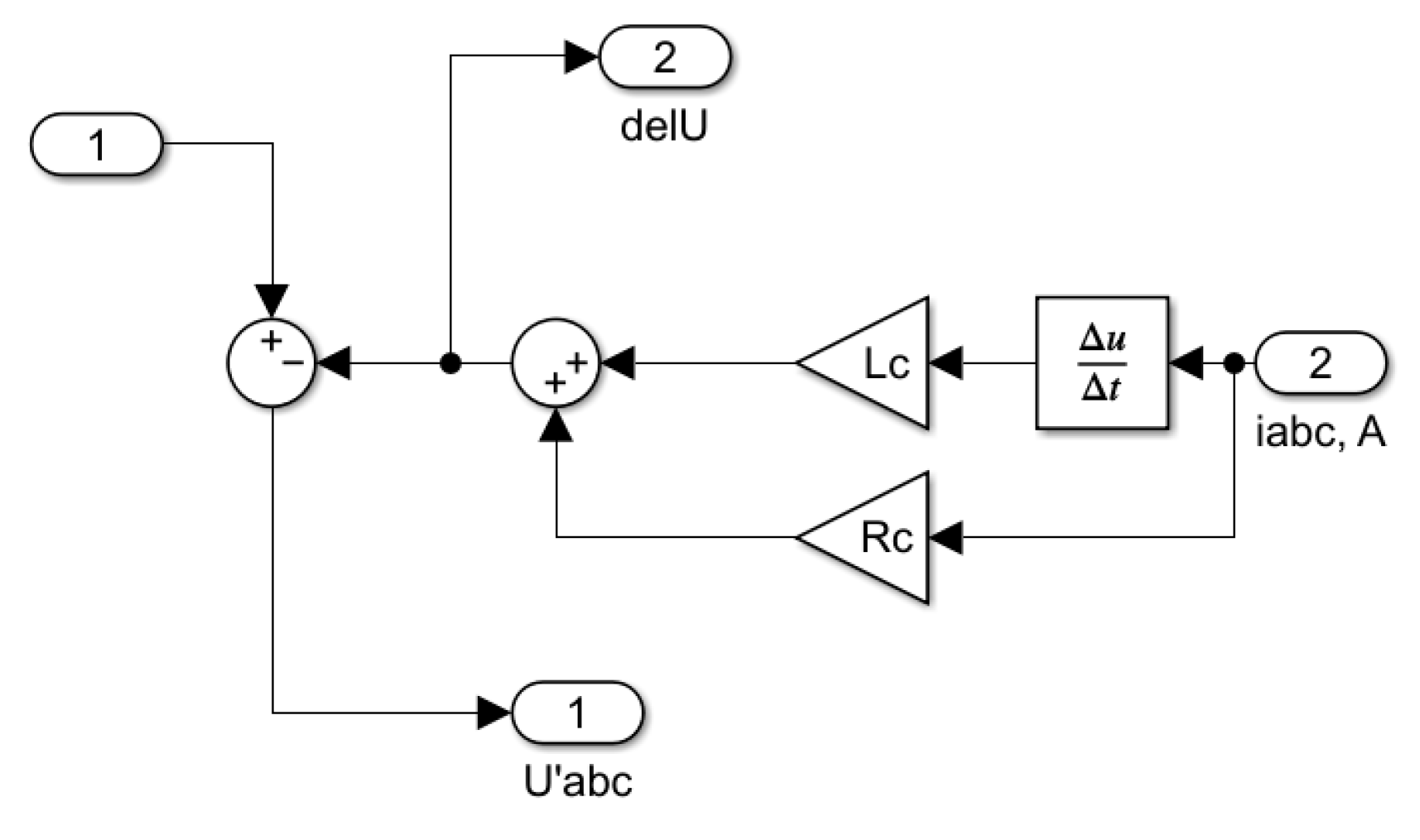
6. The Model of the Cable

For modeling, a copper cable with lengths of l = 0, 100, 300 and 500 m and a cross section of 1.5 mm² was adopted. ρ_rcu = 0.0225 Ohm∙mm²/m is the specific resistance of copper; λ_lcu = 0.08 mOhm/m is the specific reactance at 50 Hz of the cable, according to [36]. Below is a calculation of the impedance components of a cable that is 100 m long:

R_c100 = ρ_rcu · l/S_c = 1.5 Ohm;

(8)

X_c100 = λ_lcu · l = 0.008 Ohm;

(9)

Assuming that the inductive reactance was calculated for 50 Hz, the cable inductance is:

L_c = X_c100/(2π∙f) = 2.55·10⁻⁵ H;

(10)

Figure 6 shows the block diagram of the cable model in the Matlab Simulink environment.

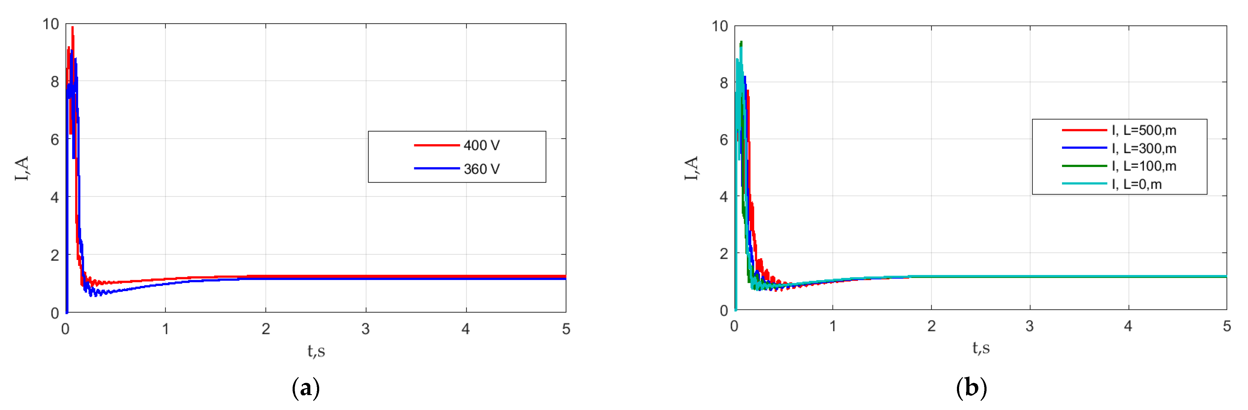
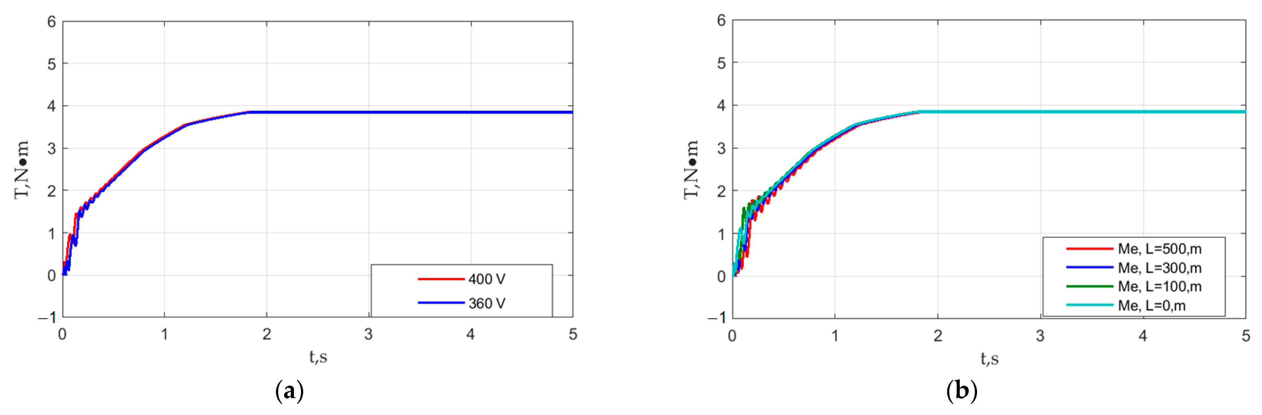
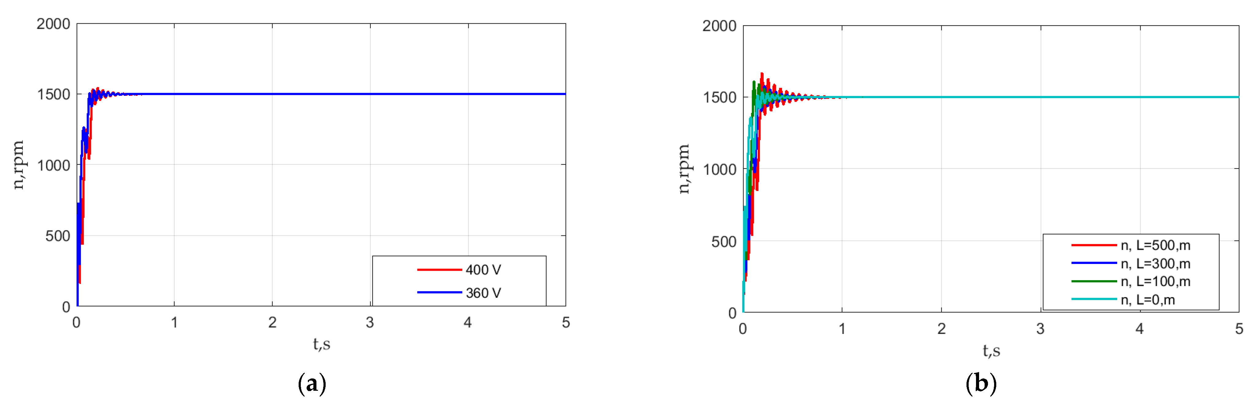
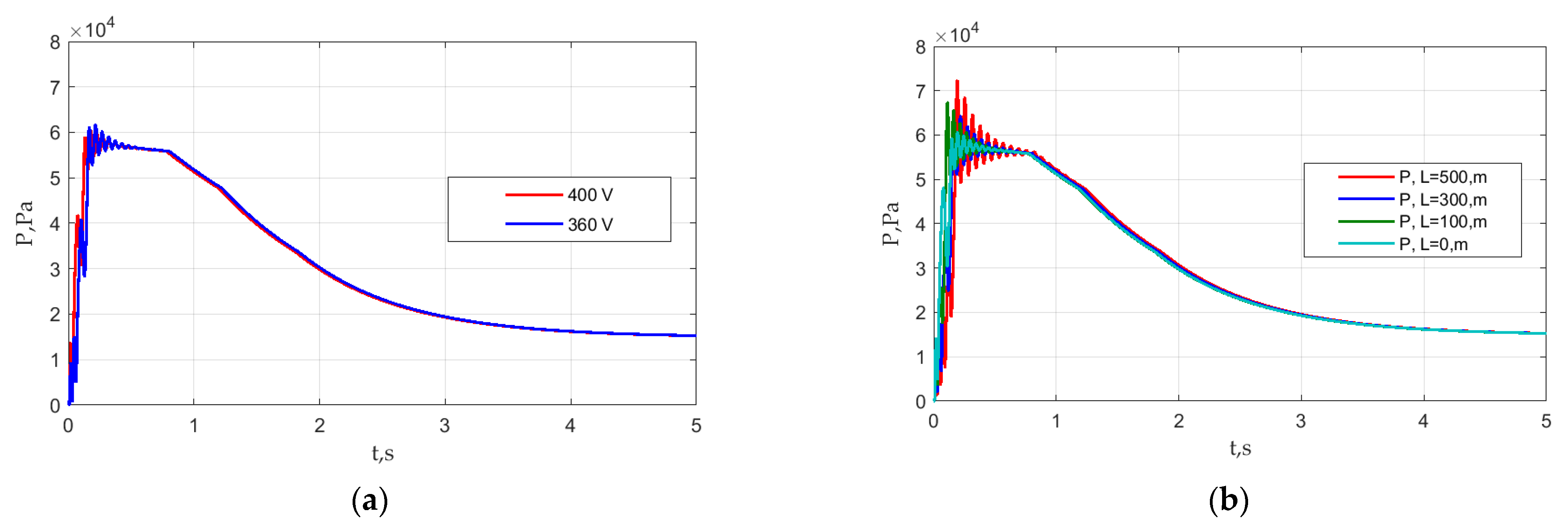
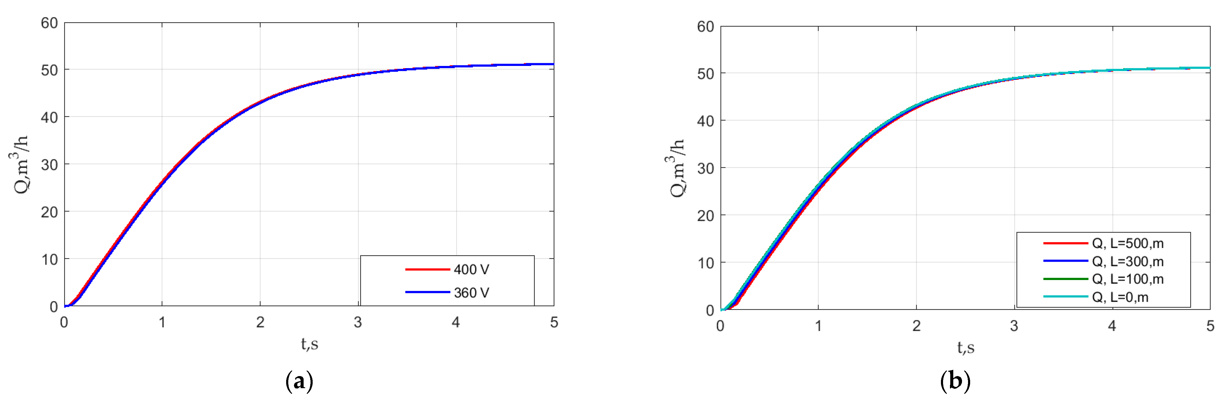
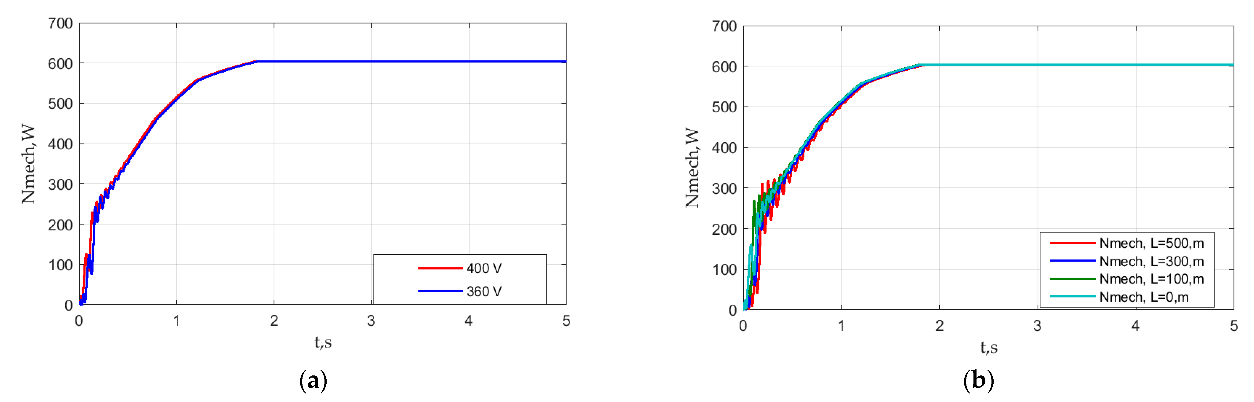
7. Simulation Results for the 0.55 kW Pump Unit

Figure 7, Figure 8, Figure 9, Figure 10, Figure 11 and Figure 12 show the results of the simulation of the electric drive of the centrifugal pump at a rated voltage of 400 V and at a voltage reduced by 10% (360 V), as well as start-up graphs for different cable lengths and the reduced voltage.

Figure 7, Figure 8, Figure 9, Figure 10, Figure 11 and Figure 12 show the instantaneous rms values of the current, the electromagnetic torque, the motor speed, the pressure, the volume flow rate and the mechanical power at the rated voltage, at a 10% reduced voltage and at a 10% reduced voltage when powered through a cable of various lengths. It can be seen from the graphs that synchronization occurs in all considered cases. Figure 9 shows that, in all the cases considered, the first achievement of the synchronous speed occurs within the time τsynch1, no more than 0.2 s, which is followed by relaxation to the synchronous speed. The characteristic time dependences of the volume flow rate on time, shown in Figure 11, are approximately τ_hydr = 2 s, i.e., much larger than τ_synch1. The dependences of the flow rate on the time in the considered cases are close to each other, since, after the synchronous speed is reached, the speed fluctuations are not large, the motor rotates at an almost synchronous speed and damped speed fluctuations have practically no effect on the flow due to hydraulic inertia. The mechanical power increases as the volumetric flow rate of the fluid increases, as can be seen in Figure 12, i.e., synchronization occurs in “soft” conditions.

As seen in Figure 7, during the starting process, the current reaches a value seven times higher than the rated one. Despite this, there are no torque surges (Figure 8). On the contrary, as the volume flow increases, the torque gradually increases, making damped oscillations, which ensures a high mechanical reliability. This behaviour of the torque is explained by a soft start and the rather small moments of inertia of the rotor and the impeller.

In some applications, such as blowers, the moment of inertia is much greater. At the same time, to facilitate starting the motor, the number of turns of the stator winding is reduced, which is equivalent to raising the voltage. Figure 7a shows that the current at the start at the reduced voltage is less than that at the rated one, which leads to the losses reduction in the winding and the increase in efficiency. So, due to the facilitated starting conditions, it is possible to recommend the manufacture of LSPMSMs for pumping applications in order to produce LSPMSMs with an increased number of turns, which is equivalent to a decrease in the supply voltage and therefore to increased efficiency.

The decrease in the current (and, therefore, the voltage) on the motor terminals in a steady state due to the presence of the cable is so small that it is not noticeable in Figure 7b. At the same time, the presence of a cable leads to a significant delay in synchronization. Thus, the effect of the cable on delaying synchronization does not come down to an equivalent decrease in the voltage/current on the motor, which is additionally explained by the generation of power by the motor into the grid at a frequency different from the frequency of the grid.

8. Parameters of the 3 kW Pump Unit

The parameters of the experimental four-pole 3 kW synchronous motor with the starting winding and permanent magnets were taken for the calculation.

Table 3. 3 kW LSPMSM parameters.

Parameter	Value
Rated power Prate, kW	3
Rated line-to-line voltage Urate, V	380
RMS rated stator current, A	5.84
Rated power factor	0.82
Rated frequency f, Hz	50
Pole pair number Zp	2
Stator phase resistance Rs, Ohm	1.281
Total direct inductance Ld, H	0.110
Total quadrature inductance Lq, H	0.0567
Leakage direct inductance Lσd, H	0.0186
Leakage quadrature inductance Lσq, H	0.0108
Rotor direct resistance r’d, Ohm	2.943
Rotor quadrature resistance r’q, Ohm	2.426
Permanent magnet flux linkage λ’0, Wb	0.6095
Motor inertia moment Jm, kg·m2	0.010
Pump impeller inertia moment Ji, kg·m2	0.0011

shows the motor parameters. The centrifugal pump “Wilo-VeroLine-IPL 100/175-3/4 28” was chosen for modeling.

Table 4. 3 kW pump characteristics.

Flow Q, m3/h	Pressure P, Pa	Power Nm, W
20.67	92,337	1613.5
40.00	91,669	1968.5
79.51	84,825	2475.3
118.96	70,390	2819.2
158.92	49,404	3011.0
188.19	30,138	3052.1

shows the pump characteristics. The pipe length l is 450 m. Its diameter D is 0.168 m.

Figure 13 shows the curves of the pressure-flow characteristics of the pump, taken at 1450 and 1500 rpm, as well as the system characteristic with an open valve.

A voltage drop on the cable is defined as a decrease in the voltage on the motor. It is possible to estimate the rms value of the voltage drop on the cable in the rated mode by the rated current and power factor [37]:

u = b∙ I ∙ (ρ_rcu ∙ L/S · cosφ+ λ ∙ sinφ);

(11)

where u is the voltage drop on the cable; b is the coefficient (1 if the circuit is three-phase and 2 if the circuit is single-phase); I is the rms value of the current; cosφ is the motor power factor. The relative voltage drop on the cable is determined as follows:

Δu = 100 u/U₀;

(12)

where U₀ is the phase voltage. The dependence of the relative voltage drop on the cable on its length is given in

Table 5. Relative cable voltage drop versus cable length.

lc, m	Δu, %
0	0
100	3.12
300	9.37
500	15.61
700	21.85

. In accordance with [37], since the voltage drop with cable lengths of 300, 500 and 700 m exceeds 4%, such cable lengths cannot be used.

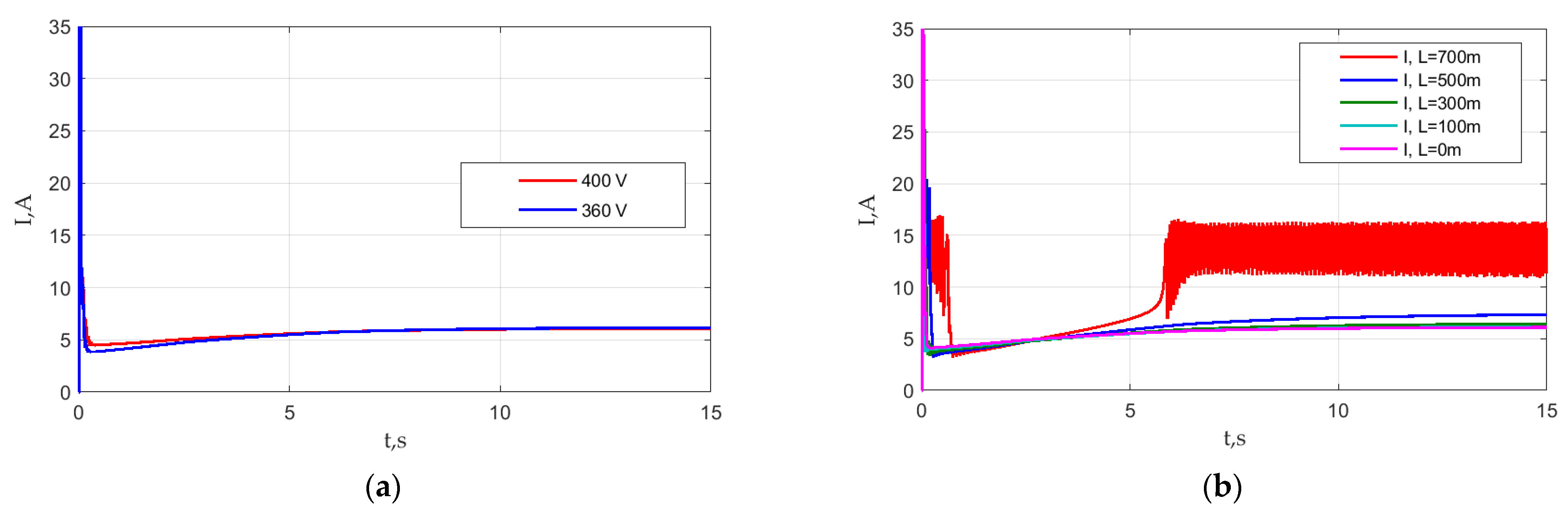
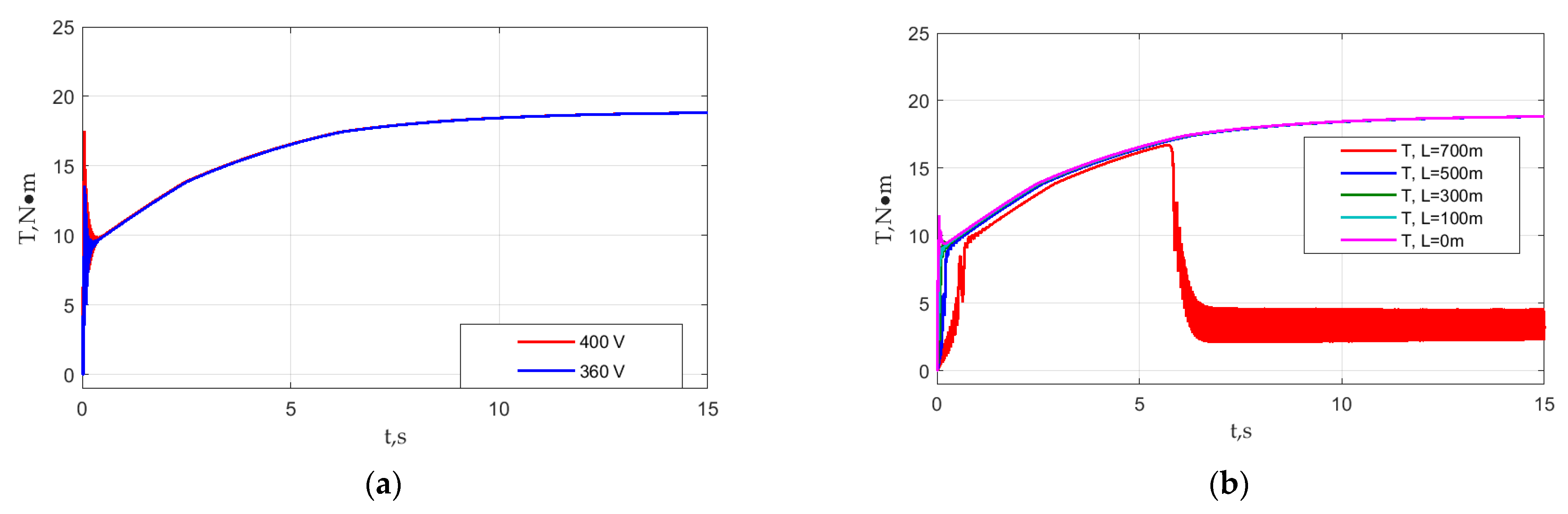
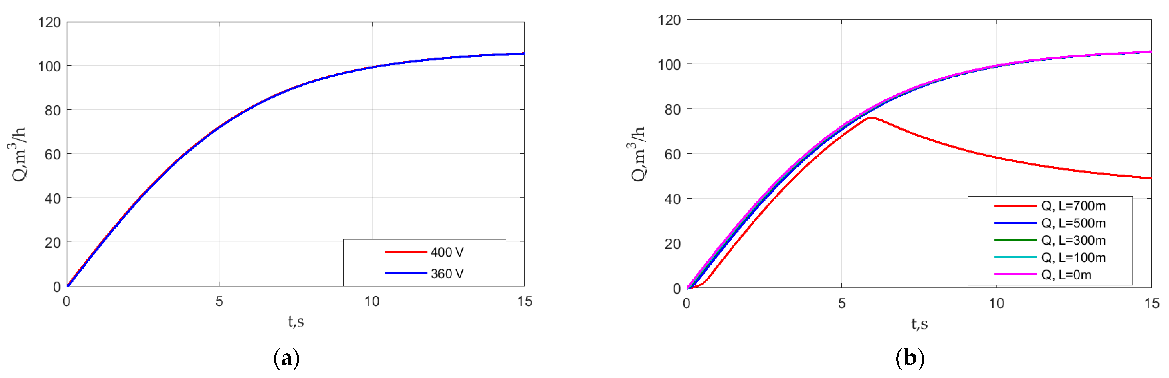
9. Simulation Results for the 3 kW Pump Unit

Figure 14, Figure 15, Figure 16, Figure 17, Figure 18, Figure 19 and Figure 20 show the results of the simulation of the pump electric drive at the rated voltage and at the voltage reduced by 10%, as well as the start-up graphs at different cable lengths and at the reduced voltage.

The results of this simulation are mainly similar to those for the 0.55 kW LSPMSM. The characteristic time of the hydrodynamic process in the pipe and in the pump is much greater than that of the mechanical and electric process in the motor. The impeller inertia is much less than that of the rotor. These result in a “soft start”. Thus, there are no torque surges exceeding the torque rated value.

Figure 14, Figure 15, Figure 16, Figure 17, Figure 18, Figure 19 and Figure 20 present the simulation results at the reduced voltage and at cable lengths of 0, 100, 300, 500 and 700 m. The standard [37] allows for a voltage drop on the cable of not more than 4%, which is satisfied only in the cases of the cable lengths of 0 and 100 m. The rest simulations are carried out to demonstrate the behavior long cables. The synchronization problems are observed only with the cable length of 700 m, which is much more than the allowed length. Namely, the synchronization occurs due to a “soft start”. However, in increasing the mechanical power, the synchronization cannot be sustained at some point.

10. Conclusions

This paper analyzes the effect of the reduced voltage and an increase in the cable length on the success of starting LSPMSM in the drive of centrifugal pump units with a power of 0.55 kW and 3 kW.

A feature of the pumps, in comparison, for example, with fans with large centrifugal masses, is that the moment of inertia of the pump impeller is several times less than the moment of inertia of the rotor itself, which makes it possible to hope that there will be no problem of unsuccessful starts of the LSPMSM in the pump drive.

The simulation examples show that, for pump drives of the considered type and power rating, the stable synchronization occurs at the rated voltage, at the voltage of 90% of the rated one and, additionally, with the supply via the cable, except for the cases in which the voltage drop in the cable significantly exceeds the level of 4% recommended in IEC 60364-5-52.

The characteristic time of the hydrodynamic process in the pipe and in the pump is much greater than that of the mechanical and electrical process in the motor. The impeller inertia is much less than that of the rotor. These result in a “soft start”. Therefore, there are no torque surges exceeding the torque rated value, which prolongs the system lifetime. Additionally, due to a “soft start”, it is expected that the number of turns of the stator winding to ensure the successful synchronization can be greater than that in other applications, which can decrease the current and increase the LSPMSM efficiency in the pump applications.

References

1. Goman, V.; Oshurbekov, S.; Kazakbaev, V.; Prakht, V.; Dmitrievskii, V. Energy Efficiency Analysis of Fixed-Speed Pump Drives with Various Types of Motors. Appl. Sci. 2019, 9, 5295. [Google Scholar] [CrossRef] [Green Version]
2. Baka, S.; Sashidhar, S.; Fernandes, B.G. Design of an Energy Efficient Line-Start Two-Pole Ferrite Assisted Synchronous Reluctance Motor for Water Pumps. IEEE Trans. Energy Conv. 2021, 36, 961–970. [Google Scholar] [CrossRef]
3. Ismagilov, F.; Vavilov, V.; Gusakov, D. Line-Start Permanent Magnet Synchronous Motor for Aerospace Application. In Proceedings of the IEEE International Conference on Electrical Systems for Aircraft, Railway, Ship Propulsion and Road Vehicles and International Transportation Electrification Conference (ESARS-ITEC 2018), Nottingham, UK, 7–9 November 2018; pp. 1–5. [Google Scholar] [CrossRef]
4. Kurihara, K.; Rahman, M. High-Efficiency Line-Start Interior Permanent-Magnet Synchronous Motors. IEEE Trans. Ind. Appl. 2004, 40, 789–796. [Google Scholar] [CrossRef]
5. Kazakbaev, V.; Paramonov, A.; Dmitrievskii, V.; Prakht, V.; Goman, V. Indirect Efficiency Measurement Method for Line-Start Permanent Magnet Synchronous Motors. Mathematics 2022, 10, 1056. [Google Scholar] [CrossRef]
6. Rotating Electrical Machines—Part 30-2: Efficiency Classes of Variable Speed AC Motors (IE-Code). IEC 60034-30-2/IEC: 2016-12. Available online: https://webstore.iec.ch/publication/30830 (accessed on 19 December 2022).
7. Quarterly Report On European Electricity Markets, Market Observatory for Energy DG Energy, 15(1), Covering First Quarter of 2022, European Commission. 2022. Available online: https://energy.ec.europa.eu/system/files/2022-07/Quarterly%20Report%20on%20European%20Electricity%20markets%20Q1%202022.pdf (accessed on 19 December 2022).
8. European Commission Regulation (EC). No. 640/2009 Implementing Directive 2005/32/EC of the European Parliament and of the Council with Regard to Ecodesign Requirements for Electric Motors, (2009), Amended by Commission Regulation (EU) No 4/2014 of January 6, 2014. Document 32014R0004. Available online: https://eur-lex.europa.eu/legal-content/EN/TXT/?uri=CELEX%3A32014R0004 (accessed on 19 December 2022).
9. European Council Meeting (10 and 11 December 2020)—Conclusions. EUCO 22/20 CO EUR 17 CONCL 8. Available online: https://www.consilium.europa.eu/media/47296/1011-12-20-euco-conclusions-en.pdf (accessed on 23 January 2021).
10. Addendum to the Operating Instructions: AC Motors DR.71.J-DR.100.J with LSPM Technology, 21281793/EN, 09/2014, SEW Eurodrive. Available online: https://download.sew-eurodrive.com/download/pdf/21343799.pdf (accessed on 19 December 2022).
11. Catalogue of Super Premium Efficiency SynchroVERT LSPM Motors. Available online: https://www.bharatbijlee.com/media/14228/synchrovert_catalogue.pdf (accessed on 19 December 2022).
12. WQuattro, Super Premium Efficiency Motor, Product Catalogue, WEG Group-Motors Business Unit, Cod: 50025713, Rev: 03, Date (m/y): 07/2017. Available online: https://static.weg.net/medias/downloadcenter/h01/hfc/WEG-w22-quattro-european-market-50025713-brochure-english-web.pdf (accessed on 19 December 2022).
13. KT-420-5, Operation of Bitzer Reciprocating Compressors with External Frequency Inverters, Bitzer, 01.2022. Available online: https://www.bitzer.de/shared_media/html/kt-420/Resources/pdf/279303819.pdf (accessed on 19 December 2022).
14. Kazakbaev, V.; Prakht, V.; Dmitrievskii, V.; Golovanov, D. Feasibility Study of Pump Units with Various Direct-On-Line Electric Motors Considering Cable and Transformer Losses. Appl. Sci. 2020, 10, 8120. [Google Scholar] [CrossRef]
15. Vasilev, B. Analysis and improvement of the efficiency of frequency converters with pulse width modulation. Int. J. Electr. Comput. Eng. 2019, 9, 2314–2320. [Google Scholar] [CrossRef]
16. Churkin, A.; Churkin, B.; Savelieva, I. Improving the energy efficiency of frequency converters in networks of limited power. IOP Conf. Ser. Mater. Sci. Eng. 2019, 643, 012056. [Google Scholar] [CrossRef] [Green Version]
17. Wang, S.-C.; Nien, Y.-C.; Huang, S.-M. Multi-Objective Optimization Design and Analysis of V-Shape Permanent Magnet Synchronous Motor. Energies 2022, 15, 3496. [Google Scholar] [CrossRef]
18. Wang, D.; Wang, X.; Chen, H.; Zhang, R. Matlab/Simulink-Based Simulation of Line-start PMSM Used in Pump Jacks. In Proceedings of the 2nd IEEE Conference on Industrial Electronics and Applications, Harbin, China, 23–25 May 2007; pp. 1179–1181. [Google Scholar] [CrossRef]
19. Paramonov, A.; Oshurbekov, S.; Kazakbaev, V.; Prakht, V.; Dmitrievskii, V. Study of the Effect of Throttling on the Success of Starting a Line-Start Permanent Magnet Motor Driving a Centrifugal Fan. Mathematics 2022, 10, 4324. [Google Scholar] [CrossRef]
20. Sethupathi, P.; Senthilnathan, N. Comparative analysis of line-start permanent magnet synchronous motor and squirrel cage induction motor under customary power quality indices. Electr. Eng. 2020, 102, 1339–1349. [Google Scholar] [CrossRef]
21. Faiz, J.; Ebrahimpour, H.; Pillay, P. Influence of unbalanced voltage on the steady-state performance of a three-phase squirrel-cage induction motor. IEEE Trans. Energy Convers. 2004, 19, 657–662. [Google Scholar] [CrossRef]
22. Gnaciński, P.; Muc, A.; Pepliński, M. Influence of Voltage Subharmonics on Line Start Permanent Magnet Synchronous Motor. IEEE Access 2021, 9, 164275–164281. [Google Scholar] [CrossRef]
23. Blair, T.H. 3 phase AC motor starting methods: An analysis of reduced voltage starting characteristics. In Proceedings of the IEEE SoutheastCon 2002 (Cat. No.02CH37283), Columbia, SC, USA, 5–7 April 2002; pp. 181–186. [Google Scholar] [CrossRef]
24. Hsu, C.-T.; Chuang, H.-J. Power quality assessment of large motor starting and loading for the integrated steel-making cogeneration facility. In Proceedings of the Fourtieth IAS Annual Meeting. Conference Record of the 2005 Industry Applications Conference, Hong Kong, China, 2–6 October 2005; pp. 59–66. [Google Scholar] [CrossRef]
25. Patil, P.; Porate, K. Starting Analysis of Induction Motor: A Computer Simulation by Etap Power Station. In Proceedings of the Second International Conference on Emerging Trends in Engineering & Technology, Nagpur, India, 16–18 December 2009; pp. 494–499. [Google Scholar] [CrossRef]
26. Low Voltage Process Performance Motors 400 V 50 Hz, 460 V 60 Hz., ABB, Catalog, February 2022. Available online: https://search.abb.com/library/Download.aspx?DocumentID=9AKK105944&LanguageCode=en&DocumentPartId=&Action=Launch (accessed on 19 December 2022).
27. International Standard IEC 60038, IEC Standard Voltages, Edition 7.0 2009-06. Available online: https://webstore.iec.ch/publication/153 (accessed on 19 December 2022).
28. Wilo, Circulation Pumps, Catalog. 2009. Available online: http://sirkulasyonpompasi.org/sirkulasyonpompasi/wilo-katalog.pdf (accessed on 19 December 2022).
29. Centrifugal Pump, Pumps and Motors. Model Description. MathWorks. Available online: https://www.mathworks.com/help/hydro/ref/centrifugalpump.html;jsessionid=9398cce96bf548d19dfefaa598e3 (accessed on 19 December 2022).
30. Fluid Inertia. Model description. MathWorks. Available online: https://www.mathworks.com/help/simscape/ref/fluidinertia.html?s_tid=doc_ta (accessed on 19 December 2022).
31. Improving Pumping System Performance, a Sourcebook for Industry. Prepared for the United States Department of Energy Office of Energy Efficiency and Renewable Energy Industrial Technologies Program, Second Edition, May 2006. Available online: https://www.energy.gov/sites/prod/files/2014/05/f16/pump.pdf (accessed on 19 December 2022).
32. Hydraulic Pipeline. Model Description. MathWorks. Available online: https://www.mathworks.com/help/hydro/ref/hydraulicpipeline.html (accessed on 19 December 2022).
33. Variable Area Hydraulic Orifice. Model Description. MathWorks. Available online: https://www.mathworks.com/help/simscape/ref/variableareahydraulicorifice.html?searchHighlight=%20hydraulic%20orifice&s_tid=srchtitle_%20hydraulic%20orifice_2 (accessed on 19 December 2022).
34. Tank. Low-Pressure Blocks. Model Description. MathWorks. Available online: https://www.mathworks.com/help/hydro/ref/tank.html?s_tid=doc_ta (accessed on 19 December 2022).
35. Estimation of Pump Moment of Inertia. Article. Native Dynamics. 10 September 2013. Available online: https://neutrium.net/equipment/estimation-of-pump-moment-of-inertia (accessed on 19 December 2022).
36. Kirar, M.; Aginhotri, G. Cable sizing and effects of cable length on dynamic performance of induction motor. Proceedings of IEEE Fifth Power India Conference, Murthal, India, 19–22 December 2012; pp. 1–6. [Google Scholar] [CrossRef]
37. IEC 60364-5-52; Electrical Installations in Buildings—Part. 5-52: Selection and Erection of Electrical Equipment—Wiring Systems, Is the IEC Standard Governing Cable Sizing. IEC: Geneva, Switzerland, 2009. Available online: https://webstore.iec.ch/publication/1878 (accessed on 19 December 2022).
Figure 1. Sketches of electric motors. (a) Induction motor (IM); (b) Line-start permanent magnet synchronous motor (LSPMSM).
Mathematics 11 00646 g001
Figure 2. Diagram of the pump unit under consideration. Here, iabc and uabc are the mains phase currents and mains voltage; ω is the mechanical angular frequency; T is the shaft torque; q is the pump volume flow rate.
Mathematics 11 00646 g002
Figure 3. Simulink model of the LSPMSM motor in the d-q axes: (a) General view of the model; (b) Calculation of stator currents; (c) Calculation of rotor currents; (d) Torque calculation.
Mathematics 11 00646 g003
Figure 4. Implementation of the model of the pump unit with the LSPMSM drive in the Matlab Simulink.
Mathematics 11 00646 g004
Figure 5. Pump head-flow curves taken at 1450 and 1500 rpm, as well as the system response with the valve open.
Mathematics 11 00646 g005
Figure 6. The block diagram of the cable model.
Mathematics 11 00646 g006
Figure 7. Motor current simulation results (envelopes of its amplitude). (a) Start with the rated and reduced voltages; (b) with the reduced voltage and different cable length.
Mathematics 11 00646 g007
Figure 8. Electromagnetic torque simulation results. (a) Start with the rated and reduced voltages; (b) Start with the reduced voltage and different cable length.
Mathematics 11 00646 g008
Figure 9. Motor speed simulation results. (a) Start with the rated and reduced voltages; (b) Start with the reduced voltage and different cable length.
Mathematics 11 00646 g009
Figure 10. Pump differential pressure simulation results. (a) Start with the rated and reduced voltages; (b) with the reduced voltage and different cable length.
Mathematics 11 00646 g010
Figure 11. Pump flow simulation results. (a) Start with the rated and reduced voltages; (b) Start with the reduced voltage and different cable length.
Mathematics 11 00646 g011
Figure 12. Pump mechanical power simulation results. (a) Start with the rated and reduced voltages; (b) Start with the reduced voltage and different cable length.
Mathematics 11 00646 g012
Figure 13. Pump head-flow curves taken at 1450 and 1500 rpm, as well as the system response with the valve open.
Mathematics 11 00646 g013
Figure 14. Motor current simulation results (envelopes of its amplitude): (a) Start with the rated and reduced voltages; (b) Start with the reduced voltage and different cable length.
Mathematics 11 00646 g014
Figure 15. Electromagnetic torque simulation results: (a) Start with the rated and reduced voltages; (b) Start with the reduced voltage and different cable length.
Mathematics 11 00646 g015
Figure 16. Motor speed simulation results: (a) Start with the rated and reduced voltages; (b) Start with the reduced voltage and different cable length.
Mathematics 11 00646 g016
Figure 17. Pump differential pressure simulation results: (a) Start with the rated and reduced voltages; (b) Start with the reduced voltage and different cable length.
Mathematics 11 00646 g017
Figure 18. Pump flow simulation results: (a) Start with the rated and reduced voltages; (b) Start with the reduced voltage and different cable length.
Mathematics 11 00646 g018
Figure 19. Rms value of the voltage drop on the cable.
Mathematics 11 00646 g019
Figure 20. Pump mechanical power simulation results: (a) Start with the rated and reduced voltages; (b) Start with the reduced voltage and different cable length.
Mathematics 11 00646 g020