Abstract
The breathing rate monitoring is an important measure in medical applications and daily physical activities. The contact sensors have shown their effectiveness for breathing monitoring and have been mostly used as a standard reference, but with some disadvantages for example in burns patients with vulnerable skins. Contactless monitoring systems are then gaining attention for respiratory frequency detection. We propose a new non-contact technique to estimate the breathing rate based on the motion video magnification method by means of the Hermite transform and an Artificial Hydrocarbon Network (AHN). The chest movements are tracked by the system without the use of an ROI in the image video. The machine learning system classifies the frames as inhalation or exhalation using a Bayesian-optimized AHN. The method was compared using an optimized Convolutional Neural Network (CNN). This proposal has been tested on a Data-Set containing ten healthy subjects in four positions. The percentage error and the Bland–Altman analysis is used to compare the performance of the strategies estimating the breathing rate. Besides, the Bland–Altman analysis is used to search for the agreement of the estimation to the reference.The percentage error for the AHN method is with and agreement with respect of the reference of ≈99%.
Keywords:
machine learning; convolutional neural networks; artificial hydrocarbon networks; Hermite transform; motion video magnification; non-contact monitoring; respiratory rate estimation; preventable death; health MSC:
68U10
1. Introduction
Respiratory Rate (RR) is a relevant vital sign used for monitoring patients in a clinical setting and also for following subjects such as the elderly during daily activities. Contact sensors have been used mostly as a standard monitoring reference proving their efficiency, but with some drawbacks. The stress, pain and irritation caused by contact in vulnerable skin in burns patients and neonates are the main inconveniences [1]. In addition, in a pandemic context, such as the recent SARS-CoV-2 pandemic, the monitoring of respiratory parameters without contact has become incontrovertible [2]. For example, Khan et al. [3] present a review including the recent non-contact sensing strategies to develop a platform to contain COVID-19.
The proposals to compute the RR using a non-contact process consist of three steps: the acquisition of the raw signal, the extraction and processing of the respiratory signal, and finally, the estimation of the RR.
There are three principal categories for the acquisition of the signal, the first group includes the non-image-based proposals, like the radar sensors approaches [4,5,6] and sound-based approaches [7]. The main weakness of these methods is that the antenna must be in front of the thoracic area, a constraint that cannot always be met [8]. For the sound-based approaches, ambient noise remains an issue for the extraction of the signal [9]. The second group includes different types of image sensing. Thermal images [10,11,12] measure the temperature oscillations between the inhalation and exhalation stages with the drawback of not working if the facial area is not visible. The remote photoplethysmography (rPPG) imaging technique, that measures the light absorption variation by the blood to track the respiratory signal by means of a camera and ambient light [13,14,15,16,17,18]. In addition to the need for the facial area to be visible, the main weakness is that the quality of the signal is low [19]. Finally, RGB images and ambient light are used to track the motion due to respiration on the thorax [20,21,22,23]. Besides, in recent works, a depth-sensing camera was used to estimate the RR and the tidal volume (TV) [24,25]. The principle is based on the computation of the depth value of the chest or abdomen during the respiratory cycle. A third category uses hybrid techniques applying different kinds of sensors. For example, [26] proposed a sleep monitoring system using infrared cameras and motion sensors. Other works combine RGB images and thermal images [27] to estimate the RR in challenging conditions as spontaneous movements of the subject.
The extraction and processing of the respiratory signal in the image approaches include methods based on tracking the motion or color variations of the video. To track the motion different methods are proposed. Massaroni et al. [21] use the subtraction of consecutive images and temporal filtering to detect the signal. Chebin et al. during a spirometry study extracted the motion of the face and the shoulders [28]. Other works tracked the subtle motions using the magnification method, detecting the invisible motions due to the respiratory rhythm [29,30,31,32,33,34]. Different methods based on tracking color changes are proposed. For example, Chen et al. [18] represent the color variations of the video using a skin reflection model. This method can be introduced to a multi-camera system for multiple persons for tracking cardio-respiratory signals [35].
The estimation of the RR, in general, is carried out directly from the respiratory signal detected in the previous step in a Region-Of-Interest (ROI) detected manually [21] or automatically [30,31] on the thorax area using peak detection or machine learning strategies as Convolutional Neural Network (CNN) [18,36] and Deep Learning [37]. Other strategies tag the frames of the video as inhalation and exhalation to estimate the RR. Al Naji et al. [38] used image processing techniques as segmentation to discriminate inhalation from exhalation frames on an ROI detected manually. In a previous work [34], we proposed the use of a CNN architecture to classify the frames as inhalations or exhalations and then to estimate the RR on the whole image. More recently [39], we reported the preliminary results of a frame classifier using a simple architecture through Artificial Hydrocarbon Networks (AHN). Insights from the latter suggest AHN is a simple but powerful predictive machine learning that reduces the computational efforts for training and implementing. In addition, literature (in different domains) recently reported some key features of AHN that make it attractive, such as a small number of hyper-parameters [40], a small number of learning parameters [41], and interpretability [42]. In this sense, the current work aims to show that an AHN model can perform in a similar but cheaper way than CNN. Furthermore, the reduction of learning parameters might be helpful for real-time and on-edge performing in future research.
In this paper, we propose a method using motion-magnified video and an AHN to classify the frames as inhalation or exhalation to extract the RR in a further process. First, the Hermite transform is used to implement the Eulerian magnification technique. Then, the tagged frames of the magnified video are used to train the AHN and it is tuned using a Bayesian optimization method. The inputs to the classifier can be the Magnified Components video (MCV) of the sequence, the Magnified Video (MV) or <the Original Video (OV). Finally, the classified tagged frames are used to compute the RR. The strategy is tested on ten subjects in four different positions (lying face down, lying face up, sitting and lying fetal). We compare the approaches to computing a percentage error regarding a visual reference of the RR. In addition, we compare the AHH classifier to a CNN optimized also by the Bayesian strategy.
The contributions of this work are: (i) the neural architecture search method for optimizing AHN and CNN models as the minimal architecture classifiers of inhalation and exhalation frames to estimate the RR, (ii) the comparative study among both models using the same conditions, and (iii) the analysis of the three different kind issues of the magnified process as inputs to the classifiers. Although our previous works [34,39] presented both simple AHN and CNN models, the architectures were manually tuned and those were not optimized. Furthermore, both models were not compared using the same conditions nor the vast set of experiments were performed, as shown in the current work. To this end, our current tagging strategy for training the CNN or the AHN uses only two classes, and it is simple to implement. The contributions and highlights regarding the mathematical side are in the context of computing methodologies for image processing: the motion magnification problem in a video, the numerical optimization of two machine learning models (AHN and CNN) and the signal detection in real acquisition conditions.
The paper is organized as follows. Section 2 presents the methodology of the proposed system including the description of the motion magnification technique, the two training strategies, and the RR measuring method. Section 3 presents the experimental protocol and the results obtained from the trained CNN. Finally, conclusions are given in the last section.
2. Materials and Methods
2.1. Dataset Creation
For this research, we recruit ten subjects (males) with a mean age of years old, mean height of cm and mean body mass of kg. All the subjects sign their consent to participate in this study. They filled out voluntarily an agreement declaring no impediment to participating with the principal investigator and the School of Engineering, considering the regulations and data policies applicable in this case. The Research Committee of the Engineering Faculty of Universidad Panamericana approved all study procedures. A dataset was elaborated to train, test and evaluate the proposed method. The acquisitions of videos were made using a CANON EOS 1300D camera. The acquisition parameters of the video sequences were a duration of 60 s, at 30 frames ( pixels) per second (fps). The ten subjects were at rest during the experiment and choose one of the following four positions: sitting (S), lying face down (LD), lying face up (LU), and lying in the fetal (LF) position. We obtained a set of 26 trials combining the ten subjects and the four positions, Table 1 shows the positions tested for each subject. The distance between the subject and the camera was approximately 1 m with an angle of 30 degrees from the horizontal line for the LD, LU and LF positions and 0 degrees for the S position, respectively. The subjects wore a t-shirt without no restrictions about the slim-fit or a loose fit of the garment. The gold standard of the RR was visually obtained from the magnified videos.

Table 1.
Positions for each subject of the dataset.
2.2. Overall Method Description
The proposed system is based on the motion magnification technique and a training-testing strategy based on a CNN and an AHN. The output of the CNN and the AHN classified the frames as inhalation (‘I’) or exhalation (‘E’) from the video sequence corresponding to the breathing signal. Finally, from the temporal labeled vector, the RR is computed. The whole system is depicted in Figure 1. We performed the training and testing stages using different data inputs and selecting AHN or CNN architectures. Black lines with straight-shaped arrows correspond to the motion magnification process and the reference signals are the tagged frames. For the training process, using the AHN or the CNN model, we previously selected one of the three data sets. The data inputs consisted of the original video (OV, green solid-line), magnified components video (MCV, blue point-dash line), and magnified video (MV, red dashed line). Finally, bold arrows perform the breath rate estimation (testing phase).
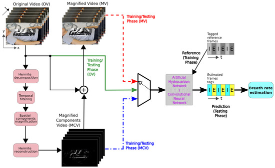
Figure 1.
Block diagram of the breath rate estimation system using the AHN or CNN model. The green solid line represents the model training using the original video (OV). The blue point-dash line uses the magnified component video (MCV). The red dashed line represents the approach using the magnified video (MV).
2.2.1. Motion Magnification
Motion magnification methods allow amplify motions in a video sequence that are imperceptible to the human eye. There are two main approaches to magnifying motion: the Lagrangian perspective and the Eulerian methods [43]. The Lagrangian approaches rely on an accurate motion estimation (e.g., optical flow methods), but with limitations such as a high computational cost and with problems handling an object’s occlusion and complex movements. As opposed, the Eulerian methods perform a spatial decomposition followed by temporal filtering in order to retain the motion components and finally add the amplified motion to the original sequence, with the advantage to have mathematically tractable models.
The Eulerian motion magnification approach amplifies a displacement function by a factor between two images and , where are the spatial coordinates and t represents the time, such that from the observed intensities we might obtain a magnified and synthesized image:
The motion magnification process first performs a spatial frequencies decomposition of the image sequence such as a first-order Taylor series would do it:
The work presented in [43] used the Laplacian pyramid as a spatial decomposition. However, in recent works, the Hermite transform (HT) has demonstrated that it performs a better reconstruction of the magnified sequence [33,44] instead of the Laplacian approach.
After spatial decomposition, a broadband temporal band filter is applied to retain the vector displacement that represents the motion component:
Spatial Decomposition
In [43], the spatial decomposition showed in Equation (3) was performed using a Laplacian pyramid, but in [33,44] it was changed by the Hermite transform, showing an improvement of the image sequence reconstruction.
The HT is an image multi-resolution decomposition model inspired by the human vision system (HVS) [45]. First, the pixel information of the image is analysed using a Gaussian window at positions that conform a sampling lattice S:
where the normalization factor is used to the unitary energy with respect to .
Then, the image information in the Gaussian window is expanded into a family of polynomials that are orthogonal to the window function.
The HT is obtained by the convolution of the image with the analysis filter bank followed by a subsampling (T) to obtain a multi-resolution transform:
with , , are the Cartesian Hermite coefficients for the analysis order m and in x and y, respectively, N is the maximum order of the expansion, and is the size of the separable analysis Hermite filter with and .
The following is a typical graphical distribution of the Hermite coefficients in the function of the order of the polynomials in the spatial directions x and y to represent the maximum decomposition order of the Hermite transform. In addition, Table 2 shows the Hermite coefficients related to the maximum decomposition order (N).
Table 2.
Hermite coefficients () related to the maximum decomposition order (N).
The analysis Hermite filters are defined by the Hermite polynomials [45]:
where the Generalized Hermite Polynomials are as follows:
In Figure 2, we show the Hermite filters with their spatial distribution, and Figure 3 shows the Cartesian Hermite coefficients with for an RGB image. Due to the RGB image being composed of three color bands, we obtained the HT only for the intensity component.
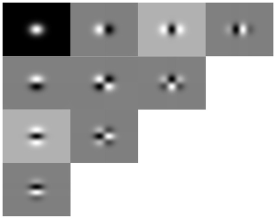
Figure 2.
The Hermite filters with and their spatial distribution .
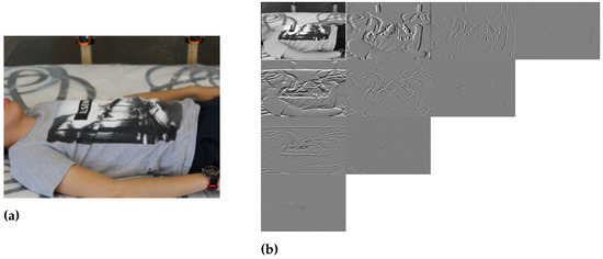
Figure 3.
(a) Example RGB image. (b) Cartesian Hermite coefficients with and spatial distribution .
To perform a perfect reconstruction of the original image a similar process is carried out using the Hermite coefficients :
where the synthesis Hermite filters are defined as follows:
with the weight function:
Motion Magnification Procedure Using the Hermite Transform
The procedure considers the following steps:
- Each RGB frame of a video is extracted and converted to an NTSC image. The NTSC image is formed by the luminance (Y) and chrominance (I and Q) values.
- A multi-resolution spatial decomposition using the forward Hermite transform is performed over each NTSC channel using the parameters , and . Figure 4 shows the Hermite coefficients for several frames of an input video, the first row shows the input frames, the second row shows the coefficient, the third and fourth rows show the and coefficient, respectively, and the fifth row shows the coefficient.
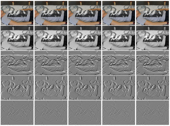 Figure 4. Hermite coefficients for several frames. Input frames (first row). coefficient (second row). and coefficients (third and fourth rows). coefficient (fifth row).
 - An ideal temporal band filter is applied in the Fourier domain to the Hermite coefficients to isolate the motion components of the spatial decomposition, where the cutting frequencies are chosen to cover a sufficiently wide range including the spectral information for any subject.
- The motion components are multiplied by the magnification factor . Figure 5 shows the magnified Hermite motion components. The first row corresponds to the Hermite motion components , the second and third rows show the Hermite motion components and , respectively, and the fourth row corresponds to the Hermite motion component .
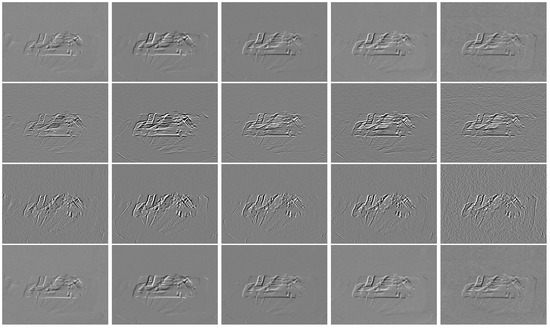 Figure 5. Magnified Hermite motion coefficients for several frames. Hermite motion components (first row). Hermite motion and (second and third rows). Hermite motion component (fourth row).
 - Using the inverse Hermite transform a reconstruction of the image sequence by the Hermite synthesis filters is carried out. The first row of Figure 6 shows several frames of the input video and in the second row, the corresponding reconstructed and magnified frames using the inverse Hermite transform are shown.
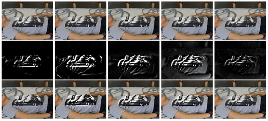 Figure 6. Several input frames (first row). Reconstructed and magnified frames using the inverse Hermite transform (second row). RGB frames’ results of the motion magnification process (third row).
 - Finally, the magnified sequence is added to the original NTSC components luma (Y) and chrominance (I and Q), and then they are converted to the RGB color space, obtaining the magnified video. The third row of Figure 6 shows the RGB frames’ results of the motion magnification process.
2.2.2. Breathing Phase Classification Using Machine Learning
Two different machine learning methods, AHN and CNN, are implemented to detect the inhalation and exhalation phases in breathing. The structures of these models are optimized to reduce their complexity and to make a fair comparison.
Artificial Hydrocarbon Networks
AHN is a supervised learning method [46] inspired by the chemical interactions and inner mechanisms of hydrocarbon compounds. The key idea of AHN is to model data accordingly to heuristic rules derived from the observations of organic compounds, obtaining a structure of data (net) comprised of packages of information [40]. In the AHN method, the latter entities are called molecules. The output of a molecule, namely , is presented in (13), where represents the carbon value, is the ith hydrogen value, is the number of hydrogen values attached to the carbon, and is the input vector with n features [40]. Moreover, a set of molecules can be interconnected among them, resulting in a structure called compound. The output of a compound can be represented by (14), where is the output of the jth molecule that approximates a subset of the inputs such that with if , and is the center of the molecule j [40]. The structure of this compound is represented in the form of , where each is a molecule in the compound. Other definitions of compounds and complex combinations of them can be found in the literature [47,48,49].
For training purposes, we adopt the so-called Stochastic Parallel Extreme (SPE-AHN) training algorithm [40]. This algorithm calculates the learning parameters, i.e., the hydrogen values H, the carbon values , and the centers of the molecules . To set up the SPE-AHN algorithm, two hyper-parameters are required: the number of molecules m in the compound and the batch size that is the percentage of training data randomly chosen by the algorithm at each iteration [40,47].
Convolutional Neural Networks
CNN is one of the most commonly used techniques in recent medical image [50]. CNNs are deep neural networks with the ability to learn complex, high-dimensional, and non-linear mappings from large collections of samples [51,52]. The CNN model normally consists of an array of convolutional layers, pooling layers, and fully-connected layers that can perform classification or regression tasks. One advantage of the CNN is the invariance to local dependency and scaling [53]. In terms of the structure, the CNN commonly combines a convolutional layer with a pooling layer performing max- or average pooling, although other strategies such as stochastic pooling and spatial pooling units are also used [54]. After a convolutional layer, the pooling layer can reduce the sensitivity of the output [55], avoiding the over-fitting and speeding up the training process [53]. These layers can be used in cascade so that the features extracted on each layer preserve only the most influential information. After that, a fully connected layer is implemented to output a response [50]. A softmax layer is commonly used at the end, to turn the output into an estimated class for classification problems [52].
Neural Architecture Search
In recent years, the paradigm for finding an optimized architecture of a neural model subjected to constraints related to complexity is called neural architecture search [56]. In a nutshell, an optimization method is used for searching the set of suitable hyper-parameters of the model. In general, this optimized set reduces the complexity of the model by setting a suitable net architecture [56].
In this work, we implement the Bayesian optimization method [57] to find the suitable values of the hyper-parameters in the models. For the AHN, we select the two hyper-parameters of the model: the number of molecules in the compound (m) and the batch size (b). For the CNN, we select the depth (n) of the net consisting of the number of convolutional layers (see Figure 7) with k filters, the fixed filter size of the convolutional layers, and the initial learning rate. The number of filters are dynamically computed by in which k decays as the depth size n is greater, as shown in [58]. Table 3 summarizes the hyper-parameters and the ranges considered in the study. The hyper-parameters were varied one at a time while the others remain in the median value, also shown in Table 3. In AHN hyper-parameters, minimum and maximum values were selected based on empirical results [40,41], while the ones in CNN were chosen from the literature evidence [50,58,59]. The initial architecture of both models is shown in Figure 7.
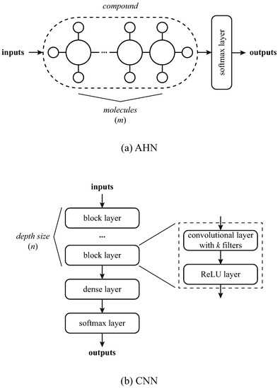
Figure 7.
Architecture prototypes of the models: (a) AHN and (b) CNN.
Table 3.
Setup of the hyper-parameters for the models. Ranges are written as (lower bound:step:upper bound).
2.2.3. Estimation of the Rate Breathing
The estimation of the respiratory rate is based on the classification of the images of the Hermite transform magnified video by the AHN or the CNN. Respiratory rate estimation is calculated using the method proposed by Brieva et al. [34] as explained next.
Once the AHN or the CNN model classifies each frame in the image sequence, and it is assigned a label inhalation (‘I’) or exhalation (‘E’), we formed a binary vector , where each label ‘I’ is changed by ‘1’ and ‘E’ by ‘0’, and M is the number of frames of the video (Figure 8).
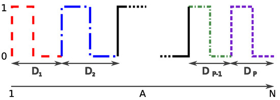
Figure 8.
Example of a binary vector A for the inhalation–exhalation cycle. corresponds to the distance (number of frames) computed from an inhalation–exhalation cycle. Each line shape and color represents a different inhalation–exhalation cycle.
From Figure 8 we can measure the distances (number of frames) that the signal takes to complete each one of the breathing cycles, e.g., from inhalation (‘1’) to exhalation (‘0’). Next, using Equation (15) we calculated an average distance as follows:
where Q is the number total of distances.
Finally, the breathing rate RR (in bpm) is computed using Equation (16):
2.3. Experiments
2.3.1. Parameters Setting
Before applying the Hermite transform-motion magnification method to the datasets, the following parameters must be defined: the size of the Gaussian window, the order maximum of the spatial decomposition, the cutting frequencies in the temporal filtering, and the amplification factor used.
For motion magnification, we used a Gaussian window of size 5 () with a maximum order of expansion of 8 (). For the temporal filtering of the Hermite coefficients, we used a band-pass filter, which was implemented through the difference between two low-pass filters, each one defined as an IIR (Infinite Impulse Response) as in [22], where the cutting frequencies for the band pass filter were fixed to 0.15–0.4 Hz corresponding to 9–24 breaths per minute. This range is sufficient to detect breathing rates in healthy subjects at rest.
2.3.2. Experimental Settings
The dataset used consists of 26 trials, each one represented by a video sequence with a duration of 60 s at 30 fps. The trials combine ten subjects and four positions: S, LD, LU, and LF, where Table 1 shows the distribution for each subject. Thus, the complete data set is composed of 46,800 images of pixels.
For the breathing phase classification, we first compute the optimized hyper-parameters of the models. We run a 5-fold cross-validation at each iteration of the Bayesian optimization method, repeating the same approach in both the AHN and the CNN models. The input size is set to of the total training data (23,400 images). The best model of each method is selected as the optimized architecture. After that, we train the optimized model using (32,760 images) of the dataset for training and (14,040 images) for testing. The four classes (positions of the subjects: S, LD, LU, and LF) are chosen in the same proportions to fulfill the training and testing sets.
The binary classification response (inhalation/exhalation) of the CNN and the AHN approaches is evaluated using the metric , where and are the true positives and true negatives, and and correspond to the false positives and false negatives, respectively. In addition, we compute the Percentage Error to evaluate the estimation of the , where the reference was obtained visually from the magnified video.
3. Results
3.1. Training of the Optimized AHN Model
We built and trained an optimized AHN model for each of the three input data strategies: OV, MV, and MCV. Table 4 summarizes the results. The reported values are the accuracy for training and testing, and the optimized values of the hyper-parameters. Furthermore, we include the total number of learning parameters (i.e., the weights in the network) required for each model. From Table 4, it is shown that the original (OV) and the magnified videos (MV) are easier to process as the number of molecules is smaller than the molecules required for the magnified components videos (MCV). Due to the number of molecules, the learning parameters are reported accordingly: 7200 weights for OV and MV, and 12,800 weights for MCV. All the input data strategies required mostly the same batch size of data (e.g., the maximum value reported is 2338 frames for MCV). The accuracy values are consistent in the training and testing revealing that the AHN models are not over-fitted. The best optimized AHN model is the one with MV as input data with a training accuracy of and testing accuracy of .
Table 4.
Training results for the AHN strategy.
3.2. Training of the Optimized CNN Model
In the same way, we built and trained an optimized CNN model for each of the three input data strategies: OV, MV, and MCV. Table 5 shows the results. The reported values are the accuracy for training and testing, and the optimized values of the hyper-parameters. We include the total number of learning parameters for each model. As depicted in Table 5, the optimized CNN models are not over-fitted because the training and the testing accuracy values are consistent between them. The results show that the CNN model with the OV input data performed the worst (training accuracy of and testing accuracy of ). The CNN model with the best accuracy values is the one with MCV input data, reporting a training accuracy of and a testing accuracy of . All the CNN models required a few convolutional layers as reported by the depth size between 2 and 3. The initial learning rate varies depending on the input strategy: 1.33E-5 (OV), 2.73E-4 (MV), and 2.30E-3 (MCV). The filter size remains 13. The learning parameters are consistent with the depth size and filter size. They reported 72,236 weights for OV, 69,708 weights for MV, and 79,858 weights for MCV.
Table 5.
Training results for CNN strategy.
3.3. Respiratory Rate Estimation Using CNN and AHN
Table 6 shows the performance of the AHN model using as input the Magnified videos (MV). The subject and his pose are listed in the first two columns. In columns three and four, the estimation (Equation (16)) and the corresponding reference are shown. Finally, column five shows the defined in Section 2.3.2. On the other hand, similarly, Table 7 shows the performance of the CNN model using the Magnified components videos (MCV). The PE is shown in the last column. Additionally, Table 8 shows the average of the in the first row for the CNN approach applied to the OV (), the MCV () and the MV () and in the second row for the AHN approach applied to the OV (), the MCV () and the MV ().
Table 6.
Performance for all the subjects of the AHN model using MV as input.
Table 7.
Performance for all the subjects of the CNN model using MCV as input.
Table 8.
for the CNN and AHN approach.
Besides, the level of agreement between the experimental results obtained by this proposal and the gold standard was estimated using the Bland–Altman method. The 95% of limits of agreements were defined as , where is the standard deviation of the MOD (mean of differences). The bias is then . In addition, the relationship between the estimated values and the reference was evaluated using Pearson’s Correlation Coefficient (PCC), the Spearman Correlation Coefficient (SCC) and the Root Mean Square Error (RMSE). For the AHN-based approach the Bland–Altman analysis is shown in Figure 9 and the statistics for the RR measurements are shown in Table 9. For the MCV strategy, a was obtained with limits of agreement of and corresponding to a bias of bpm and statistics , , and . For the MV strategy was reach a with limits of agreement of and corresponding to a bias of and statistics of , and . Finally, for the OV strategy, a was obtained with limits of agreement and corresponding to a bias of and statistics of , and . The Bland–Altman plots for the CNN-based approach are shown in Figure 10 and the statistics for the RR measurements are shown in Table 9. For the MCV strategy, a was obtained with limits of agreement of and corresponding to a bias of bpm and statistics , , and . For the MV strategy was reach a with limits of agreement of and corresponding to a bias of and statistics of , and . Finally, for the OV strategy, a was obtained with limits of agreement and corresponding to a bias of and statistics of , and . When the results are compared between the two strategies, with the use of the AHN-MV, the higher correlation (, ) is obtained, along with the smallest error () and the least limits of agreement ( and ), and with the use of CNN-MCV, the higher correlation (, ) along with the smallest error () and the least limits of agreement ( and ). Figure 11 shows the histograms overlapping of the MOD for the two architectures (AHN and CNN) for the three strategies: MCV in Figure 11a, MV in Figure 11b and OV Figure 11c. The bin centers of the histogram are defined as [) … 0 … ) )] where is chosen as the lesser value between the obtained value for the two architectures for each strategy. It is observed from the histograms that the better architecture is AHN using the strategy MV and CNN using the MCV strategy.
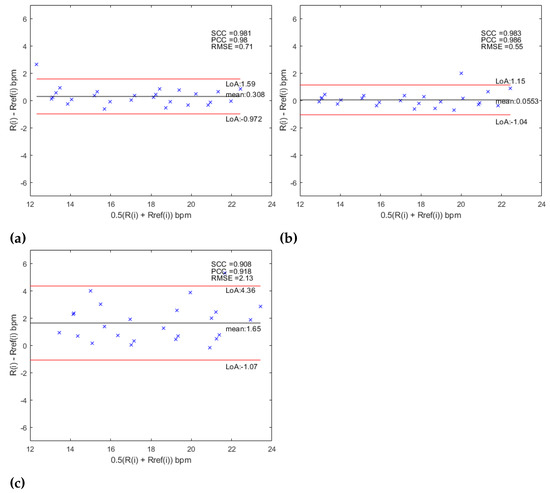
Figure 9.
Bland–Altman analysis for (a) AHN-MCV, (b) AHN-MV and (c) AHN-OV.
Table 9.
Bland–Altman metrics, correlation metrics (SCC and PCC) and RMSE for CNN and AHN strategies.
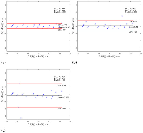
Figure 10.
Bland–Altman analysis for (a) CNN-MCV, (b) CNN-MV and (c) CNN-OV.
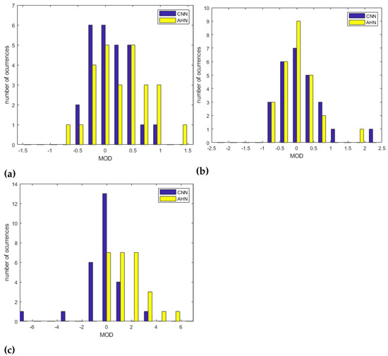
Figure 11.
Overlapped histograms of MOD for AHN and CNN architecures for the strategies (a) MCV, (b) MV and (c) OV.
Concerning the position of the subject, Table 10 shows the bias issue from the Bland–Altman Analysis and the corresponding statistics. In this sense, we compare the CNN-MCV strategy to the AHN-MV corresponding to the better results obtained using the CNN and the AHN-based approach, respectively. For the ‘LU’ position, a bias of bpm with statistics , and was obtained for the CNN-MCV strategy and a bias of bpm with statistics , , and for the AHN-MV strategy. For the ‘LF’ position, a bias of bpm with statistics , and was obtained for the CNN-MCV strategy and a bias of bpm with statistics , , and for the AHN-MV strategy. For the ’S’ position, a bias of bpm with statistics , and was obtained for the CNN-MCV strategy and a bias of bpm with statistics , , and for the AHN-MV strategy. For the ’LF’ position, a bias of bpm with statistics , and was obtained for the CNN-MCV strategy and a bias of bpm with statistics , , and for the AHN-MV strategy. By comparing results, it is observed that the less RMSE, the less bias is obtained for the ’S’ and ’LD’ positions using both strategies. Using AHN-MV, for the ’S’ position we obtained a and a . For the ‘LD’ position we obtained and a ). Using CNN-MCV, for the ‘S’ position a and a . For the ‘LD’ position and a ). Figure 12a–d shows the overlapped histograms for CNN-MCV and AHN-MV strategies for all positions. Figure 12e shows the overlapped histograms for all the subjects for CNN-MCV and AHN-MV strategies. Observing the histograms, it is observed that better results are for the ‘S’ position and ´LD´ position for both strategies. Comparing all the subjects, the obtained results are equivalent except for some outliers resulting in the AHN-MV strategy.
Table 10.
Bland–Altman metrics, correlation metrics (SCC and PCC) and RMSE for CNN and AHN strategies according to the position of the subject.
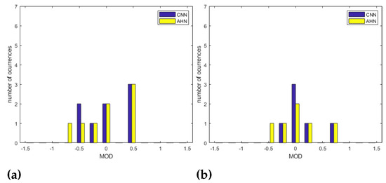
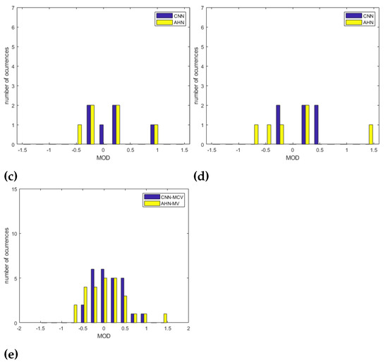
Figure 12.
Overlapped histograms of MOD for AHN-MV and CNN-MCV strategies for (a) ‘LD’ position, (b) ‘S’ position, (c) ‘LF’ position and (d) ‘LU’ position. In (e) Overlapped histograms of MOD for AHN-MV and CNN-MCV strategies for all the subjects.
4. Discussion
The system achieves measure the RR for subjects at rest in all the proposed positions. We observe that using the MV strategy training the AHN, the estimation was in good agreement (≈99%, ) with the reference obtained by visual counting in contrast to the MCV, where the agreement fell to ≈98% () and to the OV strategy, where the agreement fell to ≈97% ( bpm). Using the CNN for the MCV strategy, the estimation was in a better agreement (≈99% ) than the MV strategy (≈98% ) and the OV strategy (≈96% ). Hence, we observed that using the AHN approach the better result corresponds to a different error concerning the reference based on the MV strategy fell to < bpm with a MAE of , while using the CNN approach using the MCV strategy is the best result fell to <±1 bpm with an MAE of . Furthermore, we observed that using the magnification process, particularly the magnifying components instead of the original video, improves the detection with the CNN approach. On the other hand, the magnified video improves the detection using the AHN approach. This behavior may be because the magnification process can produce artifacts in the video, but if we take only the magnified components, the presence of these artifacts is minimized. Thus, the AHN approach is more robust when there is the presence of these artifacts. The results obtained are consistent with the fact that AHNs are better at recognizing information at the pixel level, while CNNs use the information at local level connectivity and object structures. One advantage of using the AHNs over using CNNs is that the optimization is simpler because of the fewer number of parameters.
The methodological context of this proposal is based on the selection of the ROI, the type of signal extracted from the video and the method used to extract the signal and estimate the RR. The methods used in other works compared to our proposal are summarized in Table 11. This work is not dependent of the choice of the ROI as opposed to automatic detection present in [18,30,31,36] and manual detection proposed in [21,38]. In this proposal, after the magnification, we classify each frame of the video as inhalation or exhalation (only two classes) by means of machine learning techniques (AHN or CNN) to later build a binary signal to estimate the RR in contrast to [18,36], for example, that estimate the RR using temporal information of the raw detected signal making the training process more complex. We optimize the parameters of machine learning methods (CNN and AHN) in contrast to [34,39] that use the same methodology without optimization of CNN and AHN. Table 12 summarizes the metrics to evaluate the different methodologies. Compared works using the Bland–Altman analysis, the work of Massaroni et al. [21] obtains an agreement of ≈98% () falling to a difference error with respect to the reference < bpm, consistent with our results. The work of Al-Naji et al. [38] obtains an agreement of ≈99% () falling to a difference error with respect to the reference <± 1 bpm, consistent with our work. The two latter methods are dependent on the choice of the ROI in contrast to our strategy, which does not require an ROI definition. In addition, our approach uses the tagged inhalation and exhalation frames as a reference for training the CNN as opposed to other strategies that use a reference obtained by means of a contact standard sensor. Comparing to the work of Brieva et al. [34] that uses a CNN without optimization to classify the frames as inhalation and exhalation and the magnification strategies used in this work obtain an agreement of ≈98% () for MCV strategy, an agreement of ≈97% () for the MV strategy and an agreement of ≈96% () for the OV strategy. In this work, the best agreement fell ≈99% compared to ≈98% in [34]. Concerning the position of the subject in [34] better results are observed in the ‘S’ and ‘LD’ positions consistent with our results. Comparing to the work of Brieva et al. [39] that use an AHN without optimization to classify the frames obtain an agreement of ≈97% (). Other metrics as and RMSE are only used to evaluate the performance of the methods (Table 12). Our proposal obtains consistent values compared to the other methodologies.
Table 11.
Principal works to estimate the respiratory rate.
Table 12.
Metrics to evaluate the estimation of the RR.
5. Conclusions
In this work, we implemented a new non-contact method based on the Eulerian motion magnification technique using the Hermite transform and a Bayesian optimized AHN to estimate the RR. We compared our proposal using a Bayesian-optimized CNN instead of the AHN. This strategy does not require any additional processing on the reconstructed sequence after the motion magnification to estimate the RR. The system was tested on all participants in different positions, in controlled conditions of acquisition including the surroundings of the subject (no ROI is necessary). The experimental results of RR were successfully estimated obtaining an agreement with respect to the reference of ≈99%. For future work, the use of less coefficients in the Hermite transform reconstruction step could be tested to study the performance of the networks. In addition, it would be interesting to test the robustness of the method to different camera distances and different kinds of scenarios. Furthermore, we would extend the exploratory analysis of the models using data augmentation for increasing robustness and for measuring the performance of these models in embedded systems.
Author Contributions
Conceptualization, J.B., H.P. and E.M.-A.; methodology, J.B., H.P. and E.M.-A.; software, J.B., H.P. and E.M.-A.; validation, J.B., H.P. and E.M.-A.; formal analysis, J.B., H.P. and E.M.-A.; investigation, J.B., H.P. and E.M.-A.; resources, J.B.; data curation, J.B.; writing—original draft preparation, J.B., H.P. and E.M.-A.; writing—review and editing, J.B., H.P. and E.M.-A.; project administration, J.B. All authors have read and agreed to the published version of the manuscript.
Funding
This research was funded by Universidad Panamericana grant number UP-CI-2022-MX-20-ING. The APC was funded by the Program “Fomento a la Investigación UP 2022”.
Institutional Review Board Statement
The Research Committee of the Engineering Faculty of Universidad Panamericana approved all study procedures.
Informed Consent Statement
Informed consent was obtained from all subjects involved in the study.
Data Availability Statement
The data are not publicly available due to the privacy of subjects’ information.
Acknowledgments
J.B., H.P. and E.M.-A. would like to thank the Facultad de Ingeniería of Universidad Panamericana for all support in this work.
Conflicts of Interest
The authors declare there is no conflict of interest.
Abbreviations
The following abbreviations are used in this manuscript:
| AHN | Artificial Hydrocarbon Network |
| CNN | Convolutional Neural Network |
| E | exhalation |
| HT | Hermite transform |
| HVS | human vision system |
| I | inhalation |
| LD | lying face down position |
| LF | lying in fetal position |
| LU | lying face up position |
| MCV | Magnified Components Video |
| MV | Magnified Video |
| OV | Original Video |
| PCC | Pearson’s Correlation Coefficient |
| PE | Percentage Error |
| RMS | Root Mean Square Error |
| ROI | Region-Of-Interest |
| rPPG | remote photoplethysmography |
| RR | Respiratory rate |
| S | sitting position |
| SCC | Spearman Correlation Coefficient |
| SPE-AHN | Stochastic Parallel Extreme |
References
- Zhao, F.; Li, M.; Qian, Y.; Tsien, J. Remote Measurements of Heart and Respiration Rates for Telemedicine. PLoS ONE 2013, 8, e71384. [Google Scholar] [CrossRef] [PubMed]
- Paules, C.I.; Marston, H.D.; Fauci, A.S. Coronavirus Infections—More Than Just the Common Cold. JAMA 2020, 323, 707–708. [Google Scholar] [CrossRef]
- Khan, M.; Zhang, Z.; Li, L.; Zhao, W.; Al Hababi, M.; Yang, X.; Abbasi, Q. A systematic review of non-contact sensing for developing a platform to contain COVID-19. Micromachines 2020, 11, 912. [Google Scholar] [CrossRef] [PubMed]
- Li, C.; Chen, F.; Jin, J.; Lv, H.; Li, S.; Lu, G.; Wang, J. A method for remotely sensing vital signs of human subjects outdoors. Sensors 2015, 15, 14830–14844. [Google Scholar] [CrossRef] [PubMed]
- Tsai, C.Y.; Chang, N.C.; Fang, H.C.; Chen, Y.C.; Lee, S.S. A Novel Non-contact Self-Injection-Locked Radar for Vital Sign Sensing and Body Movement Monitoring in COVID-19 Isolation Ward. J. Med. Syst. 2020, 44, 177. [Google Scholar] [CrossRef] [PubMed]
- Lee, W.; Lee, Y.; Na, J.; Kim, S.; Lee, H.; Lim, Y.H.; Cho, S.; Cho, S.; Park, H.K. Feasibility of non-contact cardiorespiratory monitoring using impulse-radio ultra-wideband radar in the neonatal intensive care unit. PLoS ONE 2021, 15, e0243939. [Google Scholar] [CrossRef] [PubMed]
- Hayashi, T.; Hirata, S.; Hachiya, H. A method for the non-contact measurement of two-dimensional displacement of chest surface by breathing and heartbeat using an airborne ultrasound. Jpn. J. Appl. Phys. 2019, 58, SGGB10. [Google Scholar] [CrossRef]
- Min, S.; Kim, J.; Shin, H.; Yun, Y.; Lee, C.; Lee, M. Noncontact respiration rate measurement system using an ultrasonic proximity sensor. IEEE Sens. J. 2010, 10, 1732–1739. [Google Scholar]
- Al-Naji, A.; Gibson, K.; Lee, S.H.; Chahl, J. Monitoring of Cardiorespiratory Signal: Principles of Remote Measurements and Review of Methods. IEEE Access 2017, 5, 15776–15790. [Google Scholar] [CrossRef]
- Mutlu, K.; Rabell, J.; Martin del Olmo, P.; Haesler, S. IR thermography-based monitoring of respiration phase without image segmentation. J. Neurosci. Methods 2018, 301, 1–8. [Google Scholar] [CrossRef]
- Schoun, B.; Transue, S.; Choi, M.H. Real-time Thermal Medium-based Breathing Analysis with Python. In Proceedings of the PyHPC 2017: 7th Workshop on Python for High-Performance and Scientific Computing, Denver, CO, USA, 12 November 2017. [Google Scholar]
- Negishi, T.; Abe, S.; Matsui, T.; Liu, H.; Kurosawa, M.; Kirimoto, T.; Sun, G. Contactless vital signs measurement system using RGB-thermal image sensors and its clinical screening test on patients with seasonal influenza. Sensors 2020, 20, 2171. [Google Scholar] [CrossRef]
- Tarassenko, L.; Villarroel, M.; Guazzi, A.; Jorge, J.; Clifton, D.A.; Pugh, C. Non-contact video-based vital sign monitoring using ambient light and auto-regressive models. Physiol. Meas. 2014, 35, 807–831. [Google Scholar] [CrossRef] [PubMed]
- Van Gastel, M.; Stuijk, S.; De Haan, G. Robust respiration detection from remote photoplethysmography. Biomed. Opt. Express 2016, 7, 4941–4957. [Google Scholar] [CrossRef] [PubMed]
- Nilsson, L.; Johansson, A.; Kalman, S. Monitoring of respiratory rate in postoperative care using a new photoplethysmographic technique. J. Clin. Monit. Comput. 2000, 16, 309–315. [Google Scholar] [CrossRef] [PubMed]
- L’Her, E.; N’Guyen, Q.T.; Pateau, V.; Bodenes, L.; Lellouche, F. Photoplethysmographic determination of the respiratory rate in acutely ill patients: Validation of a new algorithm and implementation into a biomedical device. Ann. Intensive Care 2019, 9, 11. [Google Scholar] [CrossRef] [PubMed]
- Bousefsaf, F.; Maaoui, C.; Pruski, A. Continuous wavelet filtering on webcam photoplethysmographic signals to remotely assess the instantaneous heart rate. Biomed. Signal Process. Control 2013, 8, 568–574. [Google Scholar] [CrossRef]
- Chen, W.; McDuff, D. DeepPhys: Video-Based Physiological Measurement Using Convolutional Attention Networks. Lect. Notes Comput. Sci. 2018, 11206 LNCS, 356–373. [Google Scholar]
- Luguern, D.; Macwan, R.; Benezeth, Y.; Moser, V.; Dunbar, L.; Braun, F.; Lemkaddem, A.; Dubois, J. Wavelet Variance Maximization: A contactless respiration rate estimation method based on remote photoplethysmography. Biomed. Signal Process. Control 2021, 63, 102263. [Google Scholar] [CrossRef]
- Wang, Y.; Hu, M.; Yang, C.; Li, N.; Zhang, J.; Li, Q.; Zhai, G.; Yang, S.; Zhang, X.; Yang, X. Respiratory Consultant by Your Side: Affordable and Remote Intelligent Respiratory Rate and Respiratory Pattern Monitoring System. IEEE Internet Things J. 2021, 8, 14999–15009. [Google Scholar] [CrossRef]
- Massaroni, C.; Lo Presti, D.; Formica, D.; Silvestri, S.; Schena, E. Non-contact monitoring of breathing pattern and respiratory rate via rgb signal measurement. Sensors 2019, 19, 2758. [Google Scholar] [CrossRef]
- Massaroni, C.; Schena, E.; Silvestri, S.; Maji, S. Comparison of two methods for estimating respiratory waveforms from videos without contact. In Proceedings of the Medical Measurements and Applications, MeMeA 2019, Istanbul, Turkey, 26–28 June 2019. [Google Scholar]
- Massaroni, C.; Venanzi, C.; Silvatti, A.P.; Lo Presti, D.; Saccomandi, P.; Formica, D.; Giurazza, F.; Caponero, M.A.; Schena, E. Smart textile for respiratory monitoring and thoraco-abdominal motion pattern evaluation. J. Biophotonics 2018, 11, e201700263. [Google Scholar] [CrossRef] [PubMed]
- Addison, P.; Smit, P.; Jacquel, D.; Addison, A.; Miller, C.; Kimm, G. Continuous non-contact respiratory rate and tidal volume monitoring using a Depth Sensing Camera. J. Clin. Monit. Comput. 2022, 36, 657–665. [Google Scholar] [CrossRef] [PubMed]
- Imano, W.; Kameyama, K.; Hollingdal, M.; Refsgaard, J.; Larsen, K.; Topp, C.; Kronborg, S.; Gade, J.; Dinesen, B. Non-contact respiratory measurement using a depth camera for elderly people. Sensors 2020, 20, 6901. [Google Scholar] [CrossRef] [PubMed]
- Deng, F.; Dong, J.; Wang, X.; Fang, Y.; Liu, Y.; Yu, Z.; Liu, J.; Chen, F. Design and Implementation of a Noncontact Sleep Monitoring System Using Infrared Cameras and Motion Sensor. IEEE Trans. Instrum. Meas. 2018, 67, 1555–1563. [Google Scholar] [CrossRef]
- Chen, L.; Hu, M.; Liu, N.; Zhai, G.; Yang, S. Collaborative use of RGB and thermal imaging for remote breathing rate measurement under realistic conditions. Infrared Phys. Technol. 2020, 111, 103504. [Google Scholar] [CrossRef]
- Liu, C.; Yang, Y.; Tsow, F.; Shao, D.; Tao, N. Noncontact spirometry with a webcam. J. Biomed. Opt. 2017, 22, 57002. [Google Scholar] [CrossRef] [PubMed]
- Al-Naji, A.; Gibson, K.; Chahl, J. Remote sensing of physiological signs using a machine vision system. J. Med. Eng. Technol. 2017, 41, 396–405. [Google Scholar] [CrossRef]
- Ganfure, G. Using video stream for continuous monitoring of breathing rate for general setting. Signal Image Video Process. 2019, 13, 95–1403. [Google Scholar] [CrossRef]
- Alinovi, D.; Ferrari, G.; Pisani, F.; Raheli, R. Respiratory rate monitoring by video processing using local motion magnification. In Proceedings of the European Signal Processing Conference, Rome, Italy, 3–7 September 2018; pp. 1780–1784. [Google Scholar]
- Alam, S.; Singh, S.; Abeyratne, U. Considerations of handheld respiratory rate estimation via a stabilized Video Magnification approach. In Proceedings of the Annual International Conference of the IEEE Engineering in Medicine and Biology Society, EMBS, Jeju, Republic of Korea, 11–15 July 2017; pp. 4293–4296. [Google Scholar]
- Brieva, J.; Moya-Albor, E.; Gomez-Coronel, S.; Ponce, H. Video motion magnification for monitoring of vital signals using a perceptual model. In Proceedings of the 12th International Symposium on Medical Information Processing and Analysis, Tandil, Argentina, 5–7 December 2016; Volume 10160. [Google Scholar]
- Brieva, J.; Ponce, H.; Moya-Albor, E. A Contactless Respiratory Rate Estimation Method Using a Hermite Magnification Technique and Convolutional Neural Networks. Appl. Sci. 2020, 10, 607. [Google Scholar] [CrossRef]
- Al-Naji, A.; Chahl, J. Simultaneous Tracking of Cardiorespiratory Signals for Multiple Persons Using a Machine Vision System With Noise Artifact Removal. IEEE J. Transl. Eng. Health Med. 2017, 5, 1–10. [Google Scholar] [CrossRef] [PubMed]
- Suriani, N.; Shahdan, N.; Sahar, N.; Taujuddin, N. Non-contact Facial based Vital Sign Estimation using Convolutional Neural Network Approach. Int. J. Adv. Comput. Sci. Appl. 2022, 13, 386–393. [Google Scholar] [CrossRef]
- Jagadev, P.; Naik, S.; Indu Giri, L. Contactless monitoring of human respiration using infrared thermography and deep learning. Physiol. Meas. 2022, 43, 025006. [Google Scholar] [CrossRef] [PubMed]
- Al-Naji, A.; Chahl, J. Remote respiratory monitoring system based on developing motion magnification technique. Biomed. Signal Process. Control 2016, 29, 1–10. [Google Scholar] [CrossRef]
- Brieva, J.; Ponce, H.; Moya-Albor, E. Non-Contact Breathing Rate Monitoring System using a Magnification Technique and Artificial Hydrocarbon Networks. In Proceedings of the 16th International Symposium on Medical Information Processing and Analysis, Lima, Peru, 3–4 October 2020; Volume 11583. [Google Scholar]
- Ponce, H.; de Campos Souza, P.V.; Guimarães, A.J.; Gonzalez-Mora, G. Stochastic parallel extreme artificial hydrocarbon networks: An implementation for fast and robust supervised machine learning in high-dimensional data. Eng. Appl. Artif. Intell. 2020, 89, 103427. [Google Scholar] [CrossRef]
- Ponce, H.; Martínez-Villaseñor, L. Comparative Analysis of Artificial Hydrocarbon Networks versus Convolutional Neural Networks in Human Activity Recognition. In Proceedings of the 2020 International Joint Conference on Neural Networks (IJCNN), Glasgow, UK, 19–24 July 2020; pp. 1–7. [Google Scholar]
- Martínez-Villaseñor, L.; Ponce, H.; Martínez-Velasco, A.; Miralles-Pechuán, L. An Explainable Tool to Support Age-related Macular Degeneration Diagnosis. In Proceedings of the 2022 International Joint Conference on Neural Networks (IJCNN), Padova, Italy, 18–23 July 2022; pp. 1–8. [Google Scholar]
- Wu, H.Y.; Rubinstein, M.; Shih, E.; Guttag, J.; Durand, F.; Freeman, W.T. Eulerian Video Magnification for Revealing Subtle Changes in the World. ACM Trans. Graph. 2012, 31. [Google Scholar] [CrossRef]
- Brieva, J.; Moya-Albor, E.; Gomez-Coronel, S.L.; Boris, E.R.; Ponce, H.; Mora Esquivel, J.I. Motion magnification using the Hermite transform. In Proceedings of the 11th International Symposium on Medical Information Processing and Analysis, Cuenca, Ecuador, 17–19 November 2015; Volume 9681. [Google Scholar]
- Martens, J.B. The Hermite Transform-Theory. IEEE Trans. Acoust. Speech Signal Process. 1990, 38, 1595–1606. [Google Scholar] [CrossRef]
- Ponce, H.; Ponce, P. Artificial Organic Networks. In Proceedings of the Electronics, Robotics and Automotive Mechanics Conference (CERMA), Cuernavaca, Mexico, 15–18 November 2011; pp. 29–34. [Google Scholar]
- Ponce, H.; Ponce, P.; Molina, A. Artificial Organic Networks: Artificial Intelligence Based on Carbon Networks. In Studies in Computational Intelligence; Springer: Berlin, Germany, 2014; Volume 521. [Google Scholar]
- Ponce, H.; Ponce, P.; Molina, A. The development of an artificial organic networks toolkit for LabVIEW. J. Computat. Chem. 2015, 36, 478–492. [Google Scholar] [CrossRef] [PubMed]
- Ponce, H.; Ponce, P.; Molina, A. Adaptive noise filtering based on artificial hydrocarbon networks: An application to audio signals. Expert Syst. Appl. 2014, 41, 6512–6523. [Google Scholar] [CrossRef]
- Sarvamangala, D.; Kulkarni, R.V. Convolutional neural networks in medical image understanding: A survey. Evol. Intell. 2021, 15, 1–22. [Google Scholar] [CrossRef] [PubMed]
- LeCun, Y.; Bottou, L.; Bengio, Y.; Haffner, P. Gradient-based learning applied to document recognition. Proc. IEEE 1998, 86, 2278–2324. [Google Scholar] [CrossRef]
- LeCun, Y.; Huang, F.J.; Bottou, L. Learning methods for generic object recognition with invariance to pose and lighting. In Proceedings of the 2004 IEEE Computer Society Conference on Computer Vision and Pattern Recognition, Washington, DC, USA, 27 June–2 July 2004; Volume 2, pp. II97–II104. [Google Scholar]
- Wang, J.; Chen, Y.; Hao, S.; Peng, X.; Hu, L. Deep learning for sensor-based activity recognition: A survey. Pattern Recognit. Lett. 2019, 119, 3–11. [Google Scholar] [CrossRef]
- Guo, Y.; Liu, Y.; Oerlemans, A.; Lao, S.; Wu, S.; Lew, M.S. Deep learning for visual understanding: A review. Neurocomputing 2016, 187, 27–48. [Google Scholar] [CrossRef]
- Zeng, M.; Nguyen, L.T.; Yu, B.; Mengshoel, O.J.; Zhu, J.; Wu, P.; Zhang, J. Convolutional neural networks for human activity recognition using mobile sensors. In Proceedings of the 6th International Conference on Mobile Computing, Applications and Services, Austin, TX, USA, 6–7 November 2014; pp. 197–205. [Google Scholar]
- Baymurzina, D.; Golikov, E.; Burtsev, M. A Review of Neural Architecture Search. Neurocomputing 2021, 474, 82–93. [Google Scholar] [CrossRef]
- Snoek, J.; Larochelle, H.; Adams, R.P. Practical bayesian optimization of machine learning algorithms. In Proceedings of the 26th Annual Conference on Neural Information Processing Systems, Lake Tahoe, NV, USA, 3–6 December 2012; pp. 2951–2959. [Google Scholar]
- Zhao, Y.; Liu, Y. OCLSTM: Optimized convolutional and long short-term memory neural network model for protein secondary structure prediction. PLoS ONE 2021, 16, e0245982. [Google Scholar] [CrossRef] [PubMed]
- Gülcü, A.; Kuş, Z. Hyper-parameter selection in convolutional neural networks using microcanonical optimization algorithm. IEEE Access 2020, 8, 52528–52540. [Google Scholar] [CrossRef]
Disclaimer/Publisher’s Note: The statements, opinions and data contained in all publications are solely those of the individual author(s) and contributor(s) and not of MDPI and/or the editor(s). MDPI and/or the editor(s) disclaim responsibility for any injury to people or property resulting from any ideas, methods, instructions or products referred to in the content. |
© 2023 by the authors. Licensee MDPI, Basel, Switzerland. This article is an open access article distributed under the terms and conditions of the Creative Commons Attribution (CC BY) license (https://creativecommons.org/licenses/by/4.0/).