Article

Phase-Space Modeling and Control of Robots in the Screw Theory Framework Using Geometric Algebra

by
Jesús Alfonso Medrano-Hermosillo
,
Ricardo Lozoya-Ponce
*,†,
Abraham Efraím Rodriguez-Mata
and
Rogelio Baray-Arana
Instituto Tecnológico de Chihuahua (ITCH), Chihuahua 31310, Mexico
*
Author to whom correspondence should be addressed.
This author contributed equally to this work.
Mathematics 2023, 11(3), 572; https://doi.org/10.3390/math11030572
Submission received: 15 December 2022 / Revised: 13 January 2023 / Accepted: 18 January 2023 / Published: 21 January 2023

Abstract

:
The following paper talks about the dynamic modeling and control of robot manipulators using Hamilton’s equations in the screw theory framework. The difference between the proposed work with diverse methods in the literature is the ease of obtaining the laws of control directly with screws and co-screws, which is considered modern robotics by diverse authors. In addition, geometric algebra (GA) is introduced as a simple and iterative tool to obtain screws and co-screws. On the other hand, such as the controllers, the Hamiltonian equations of motion (in the phase space) are developed using co-screws and screws, which is a novel approach to compute the dynamic equations for robots. Regarding the controllers, two laws of control are designed to ensure the error’s convergence to zero. The controllers are computed using the traditional feedback linearization and the sliding mode control theory. The first one is easy to program and the second theory provides robustness for matched disturbances. On the other hand, to prove the stability of the closed loop system, different Lyapunov functions are computed with co-screws and screws to guarantee its convergence to zero. Finally, diverse simulations are illustrated to show a comparison of the designed controllers with the most famous approaches.

1. Introduction

In the Lagrangian approach, the two fundamental variables, written as position ( θ ) and velocity ( θ ˙ ), are mutually dependent. However, in the Hamiltonian formalism, the fundamental variables, computed as position ( θ ) and momentum (p), provide more abstract and profound formulations mechanics [1]. For example, Hamiltonian formalism is very important in the study of the energy changes that are possible in molecules and atoms. In addition, it is crucial if it is interested in quantizing a dynamical system or in quantum theory. Thus, this field should be taken into account [1,2].
The Lagrangian formalism (traditionally used in robots) is based on the kinetic and potential energies of the robot. This function is used to construct the body dynamics and then the control of the system [3]. Therefore, the resulting dynamic model and its controller will be represented by positions and velocities. However, in robotics, it is possible to compute controllers using Hamiltonian formalism, because the momenta, in theory, change very quickly (in rate 1/10) [4]. In addition, in practice, it is easier to measure these forces with sensors. Hence, there are motivations to implement controllers using the Hamiltonian approach. Some relevant works about Hamiltonian controllers are mentioned below.
In [5], the authors present a proportional-derivative control with gravity compensation (PD+G) using Hamilton’s equations for robot manipulators with multiple degrees of freedom, demonstrating and proving the analysis using a simulation for a planar robot. In [6], the authors propose a hybrid controller for a SCARA robot. The work is based on a port-controlled Hamiltonian system to reduce the position tracking error. In [7], using Hamilton’s equations, the work describes a formalism to control electromechanical systems. On the other hand, there are other advanced works formulating Hamiltonian mechanics using a geometric framework. In [8], the work proposes Hamiltonian mechanics in terms of Geometric Calculus, where the author mentioned that their Hamiltonian formalism would be highly important for application with robots. On the other hand, other works are using GA to reduce the computational cost, as mentioned in [9]. In [10], geometric algebra is utilized to compute Hamiltonian mechanics and the Poisson bracket, where this work could be used in robotics. The authors in [11] illustrate the importance of Hamiltonians in robotics. The technique computes the dynamic equations using Newton–Euler and describes the local Hamiltonians in each joint to implement its law of control. Based on the above, the Hamiltonian equations can be used to control electromechanical systems. However, the previous works have been developed using the traditional Euler–Lagrange or Newton–Euler equations, where in some robots, the computational cost is high due to the considerable multiplications between the diverse components. In addition, the development is tedious for some robots. Hence, the new proposed method expands the Hamiltonian control approach using screw theory, where this powerful mathematical tool has been used in recent years for the analysis of spatial mechanisms and some works have expressed it as “the forgotten tool in multibody dynamics” [12,13].
Screw theory is a mathematical tool for the analysis of spatial mechanics, the main element of this theory is the screw [14]. The screw is constructed by two three-dimensional vectors, where these vectors are angular velocity and linear velocity [15,16]. Therefore, it is possible to study rigid bodies using this technique. The screw theory has gained importance because it is an elegant mathematical tool and can reduce the number of multiplications between the Lie group S E ( 3 ) (as is common in traditional techniques) [17]. Moreover, some authors describe the analysis of the kinematics and dynamics of rigid bodies using screw theory as modern robotics [18]. In robotics, several works using screw theory have gained prominence in recent years. For example, diverse authors propose the screw theory approach in the process of inverse and/or forward kinematics [19,20,21,22]. Other relevant techniques are described below. In [23], the paper describes an analysis of error sources of industrial robots, where they proposed a pose error model of industrial robots with screw theory. In [24], the authors propose a mathematical model using Kane’s dynamic equations in the framework of screw theory. In [25], they study the rigid-body dynamics of serial robots subject to time-invariant holonomic constraints on their end-effectors. The paper proposes a technique to compute the dynamic model of robots in the framework of screw theory. On the other hand, other interesting approaches for the dynamic models are mentioned in [26,27]. Alternatively, in [28], the method suggests a motion control approach with a focus on robotic manipulators based on screw theory and dual quaternions, where they add a stability analysis to propose a law of control for a desired trajectory. However, the drawback is that, while previous works consider kinematics and dynamics in rigid bodies, controllers are not directly proposed using screw theory. Therefore, it is an interesting motivation to compute controllers using the screw theory and the Hamiltonian approach. In addition, GA is proposed to compute the screws of the controllers and dynamics of the system; this novel approach reduces the number of operations and is intuitive for new researchers in the robotics field (due to previous knowledge of vector calculus not being required).
Taking into account the previous literature, it is possible to see that the Hamilton’s equations can be used as a methodology to compute controllers for robots, where our work extends these equations for robots in the screw theory framework and iteratively. In addition, GA is proposed for computing the diverse screws and co-screws, which is an advantage for new users interested in robotics. Regarding the controllers, the equations of the robot are designed with co-screws and screws using the approach in [17]. Later, to prove convergence, functions with screws and co-screws are computed to satisfy the Lyapunov theory and thus obtain the law of control. The main advantages of our approach are:
- Due to the use of GA, vector calculus knowledge is not required [29,30].
- Using the screw theory, the Denavit–rtenberg (D–H) representation and the homogeneous matrices are avoided. It is well known that with the traditional method, it is possible to have multiple results (this is due to the D–H technique). The above could be a risk of confusion by different designers [20].
- As the proposed technique is iterative, it is possible to be implemented in serial robots with any degrees of freedom. In addition, the Euler–Lagrange and Newton–Euler methods are avoided. Therefore, robot dynamics and control can be computed easily.
- Due to the laws of control being computed directly using screw theory, they are intuitive and can be programmed easily.
- Using sliding mode control, the robustness of the system under matched perturbations is obtained [31].
The document is organized as follows: In Section 2, we illustrate the theoretical bases of geometric algebra. In Section 3, the mathematical development necessary to construct the controllers is presented. In Section 4, we show the laws of control and their stability. In Section 5, we present a numerical example with a simulation to prove the designed located controllers. Finally, in Section 6, we illustrate the conclusions.

2. Geometric Algebra

In mathematics, geometric algebra is a term applied to Clifford’s theory of algebras [29,32]. The GA of an n-dimensional space is denoted by G p , q , r , where p , q and r represent the orthonormal basis vectors that square to 1 , 1 and 0, respectively. On the other hand, in additional to scalar multiplication and vector addition, GA is endowed with a noncommutative product, this product is the Clifford product (or geometric product). For example, the Clifford product for two vectors a , b are:
a b = a · b + a b
In Equation (1), the right side illustrates two elements: the first one is the inner product or dot product (symmetric part); the second one is the wedge product or exterior product (antisymmetric part), where the wedge product is a distributive, associative, and anti-commutative operator. The elements computed by the exterior product of k independent vectors span the k-th exterior power. In this space, each element is called a k v e c t o r . The diverse multi-vectors are entities computed by the sum of elements of the set of G n , written as:
A = A 1 + A 2 + . . . + A n
In addition to Equation (2), contemplate two homogeneous multi-vectors A and B of grade r and s, respectively. The Clifford product can be shown as:
A B = A B r + s + A B r + s 2 + . . . + A B | r s |
where A B t , indicate the t-grade part of the multi-vector A B . Suppose a n-dimensional space with diverse orthonormal basis vectors { e i } , i = 1 , , n , such that e i · e j = δ i , j , where δ i , j = 1 | i = j and δ i , j = 0 | i j . The basis vectors for the entire GA are:
{ 1 ; e i ; e i e j ; e i e j e k ; · · · ; I = e 1 · · · e n }
where I is called the pseudoscalar. Below, we include some important definitions that are useful in geometric algebra, for details consult [8,29,32,33].
Definition 1.
Let a multi-vector A of grade r. After, the reverse of A, written as A ˜ , is defined by:
A ˜ = i = 0 r ( 1 ) i ( i 1 ) 2 A i
Definition 2.
Let a multi-vector A of grade r. After, the Clifford conjugate of A, written as A ¯ , is defined by:
A ¯ = i = 0 r ( 1 ) i ( i + 1 ) 2 A i
Definition 3.
Let a G 3 . The rotation of a, written as a , is defined by the following versor product:
a = R θ a R θ ˜ = e θ 2 L a e θ 2 L
where R θ is the rotor operator, θ is the rotation angle, and L is the Lie algebra generator. The 2-vector L is the operator of rotation used in quaternions; in a different way, just consider e 2 e 3 i , e 3 e 1 j and e 1 e 2 k .
Definition 4.
Let I G n . After, the inverse of I, written as I 1 , is defined by:
I 1 = I ˜ I I ˜
Definition 5.
Let a multi-vector A of grade r. After, the dual of A, written as A * , is defined by:
A * = i = 0 r A i I 1
Definition 6.
Consider two homogeneous multi-vectors A and B. After, the commutator product between A and B is defined by:
A × ̲ B = 1 2 ( A B B A )
Definition 7.
Consider two homogeneous multi-vectors A and B. After, the anti-commutator product between A and B is defined by:
A × ¯ B = 1 2 ( A B + B A )

3. Mathematical Development

3.1. Screws

Suppose the following Lie group:
S E ( 3 ) : = R x 0 1 : R S O ( 3 ) , x R 3
The Lie algebra of S E ( 3 ) is:
s e ( 3 ) : = w v s . 0 0 : w s o ( 3 ) , v s . R 3
where s e ( 3 ) , w and v represent the Lie algebra of the Lie group S E ( 3 ) , the angular velocity, and the linear velocity, respectively [18]. On the other hand, the Lie algebra elements are often illustrated as follows:
s = w v s .
where s is constructed by two three-dimensional vectors called screws.

Lie Algebra Elements

Consider a path through the identity ( e ) in a group ( G ) :
γ : R G
where γ ( 0 ) = e . The Lie algebra element is calculated by following a path γ ( t ) starting at the identity element of S E ( 3 ) and evaluating d d t | t = 0 γ ( t ) [14,17]. Therefore, suppose the following path:
t = x R θ x R θ ˜
where t is the translation vector. After, computing the Lie algebra element:
v = d d t R θ x R θ ˜ + R θ x d d t R θ ˜
Considering d d t R θ = θ ˙ 2 L R θ and d d t R θ ˜ = θ ˙ 2 L R θ ˜ :
v = θ ˙ 2 L R θ x R θ ˜ + R θ x θ ˙ 2 L R θ ˜
Now, evaluating around the entity, where R θ ( 0 ) = R θ ˜ ( 0 ) = 1 :
v ( 0 ) = 1 2 x L L x θ ˙
Finally, using Definition 6:
v ( 0 ) = L × ̲ x θ ˙
Therefore, the linear velocity is the commutator between the Lie algebra generator of the rotor and the point x. On the other hand, the angular velocity is solved using the same methodology. The path through the identity is γ ( t ) = R θ , where R θ ( 0 ) = 1 and R θ R θ ˜ = 1 . Differentiating the last relation:
d d t R θ R θ ˜ + R θ d d t R θ ˜ = 0
Now, evaluating around the entity:
L θ ˙ L θ ˙ = 0
Hence, the Lie algebra element consists of a 2 v e c t o r L. In consequence, the angular velocity is expressed by the Lie algebra generator of the rotor. However, traditionally, the angular velocity is written as a unit vector [34,35,36]. Thus, this notation can be used by Definition 5. Therefore, the angular velocity is:
w ( 0 ) = L * θ ˙
Finally, with our approach, the screw described above can be written as:
s ( 0 ) = L * L × ̲ x θ ˙
It is possible to see that each screw can be computed easily with the previous equation. In each DoF, it is only necessary to record the Lie algebra element and its Cartesian position.

3.2. Velocity Kinematics

In robotics, the screws express the velocities of the diverse joints, where the velocity for a robot with n degrees of freedom (DoF) can be illustrated by:
V n ( 0 ) = j = 1 n s j ( 0 ) θ j ˙
where the previous velocity is only valid in the identity or in the home position. To find the velocity in the current position of the robot, it is necessary to compute the current screw ( s ) . To write the current screw, it is indispensable to use the following notation:
s j = e θ i a d ( s i ) s j ( 0 ) θ ˙
Here, we use the adjoint representation and the exponential mapping to compute the current screw [37]. Therefore, the velocity of a serial robot with n DoF, in any position, is:
V n = j = 1 n s j θ j ˙
From Equation (27), you can see that the different screws are the columns of the Jacobian matrix in robotics.

3.3. Co-Screws

Properly speaking, co-screws are linear functional on the velocities, satisfying the following:
F : s e ( 3 ) R w h e r e F ( a s 1 + b s 2 ) = a F ( s 1 ) + b F ( s 2 )
Here, a , b R , and F ( s ) are often called the evaluation map. The co-screws are constructed using two three-dimensional vectors, but, contrary to screws, these elements are computed by the dual Lie algebra s e * ( 3 ) . Thus, in robotics, the momentum co-screw ( P ) can be written as follows:
P = j p
where j and p represent the angular and linear momentum, respectively, [17]. Furthermore, the evaluation map is illustrated as:
P ( V ) = P T V
Another choice to construct the momentum co-screw is using the inertia operator, where the inertia provides an isomorphism as:
N : s e ( 3 ) s e * ( 3 )
and it is computed by:
N = e θ i a d T ( s i ) N ( 0 ) e θ i a d ( s i ) a n d N ( 0 ) = I m C m C T m I 3
Here I represents the inertia tensor, m the mass of the link, C the adjoint representation of the center of mass and I 3 the identity matrix in R 3 . Hence, the momentum co-screw can be written as [17]:
P = N V

3.4. Lagrangian Formulation of Dynamics Using Screw Theory

The kinetic energy can be described, in the context of the screw theory, as a combination of the momentum co-screw and the screw:
E k θ , θ ˙ = j = 1 n 1 2 j j · w j + p j · v j = j = 1 n 1 2 P j ( V j ) = j = 1 n 1 2 N j V j ( V j )
Using the evaluation map, Equation (34) changes to:
E k θ , θ ˙ = j = 1 n 1 2 V j T N j V j
On the other hand, the potential energy is written by:
E p θ = j = 1 n g ˜ T c ˜ j
where:
g ˜ = g e 2 0 c ˜ j = m j c j m j
Here, g is the gravitational force, m j is the mass of each link and c j is the position of the center of mass. Then, using the Euler–Lagrange equation, it is computed the dynamic equations of the robotic system (for details see the Appendix A). Therefore:
τ i = d d t L θ , θ ˙ , t θ ˙ i L θ , θ ˙ , t θ i
where:
d d t L θ , θ ˙ , t θ ˙ i = j = i n s i T N j V ˙ j + V j T N j s i , V j + V j T N j V i , s i
L θ , θ ˙ , t θ i = j = i n G j T s i V j T N j s i , V i
Therefore, the robot dynamics are described by:
τ i = j = i n V ˙ j T N j s i + V j T N j s i , V j G j T s i
where G is the co-screw of the gravitational forces and s i , V j is the Lie bracket [17,25].

3.5. Hamilton’s Equations

Hamilton’s equations can be computed using the Legendre transformation [1]:
H θ , p , t = i = 1 n p i θ ˙ i L θ , θ ˙ , t
where the partial derivation with respect to p i provides:
H θ , p , t p i = θ ˙ i
The previous equation is one of Hamilton’s equations. To compute the second equation is necessary to use the partial derivation of Equation (42) with respect to θ i :
H θ , p , t θ i = L θ , θ ˙ , t θ i
Finally, the third Hamilton’s equation is computed using Equation (38) with Equation (44) and p i = L θ , θ ˙ , t θ ˙ i :
p ˙ i = τ i H θ , p , t θ i

4. Hamilton Control Using Screw Theory

With our approach using screw theory, Hamilton’s equations can be written as (for details see Appendix A):
H θ , p , t p i = θ ˙ i
H θ , p , t θ i = j = i n P j T s i , N i 1 P i G j T s i
p ˙ i = τ i + j = i n G j T s i P j T s i , N i 1 P i
The previous equations could be used to compute the dynamic equations of robots in the phase space. After, to ensure that the robot reaches the desired position using the Hamiltonian approach, it is necessary to consult the following theorems.
Theorem  1.
A serial robot system reaches a desired position using the following control law:
τ i = K i s i g n ( S i ) + K S i S i H θ , p , t p i j = i n P j T N i 1 P i , s i G j T s i
where S i = p ˜ i + θ ˜ i is the sliding surface, p ˜ i = p d i p i is the error between the desired and measured momentum, θ ˜ i = θ d i θ i is the error between the desired and the measured joint position, and K i , K S i R + .
Proof. 
In sliding mode control, the convergence of the surface needs to be satisfied [38]. Hence, the following Lyapunov function is proposed:
V ( S i ) = 1 2 S i × ¯ S i
Now, use Definition 7 and differentiate the Lyapunov function in terms of time:
V ( S i ) ˙ = S i × ¯ S i ˙ = S i × ¯ d d t p ˜ i + θ ˜ i
Using θ ˜ i ˙ = θ ˙ i , Equations (46) and (48):
V ( S i ) ˙ = S i × ¯ τ i j = i n P j T N i 1 P i , s i G j T s i H θ , p , t p i
Applying the controller in Equation (49):
V ( S i ) ˙ = K i | S i | K S i S i × ¯ S i
Thus, as the derivative of the Lyapunov function is negative definite, the convergence of the sliding surface is satisfied. Then, S i = 0 θ ˜ i = 0 . Hence, the serial robot with the proposed controller will reach the desired position [38]. On the other hand, the closed-loop system can be computed applying Equation (49) into Equation (48):
p ˜ ˙ i = H θ , p , t p i K i s i g n ( S i ) K S i S i
Theorem  2.
A serial robotic arm will track a desired smooth function by applying the following law of control:
τ i = K p i θ ˜ i + K v i p ˜ i + p d ˙ i j = i n P j T N i 1 P i , s i G j T s i
where S i = p ˜ i + θ ˜ i is the sliding surface, p ˜ i = p d i p i is the error between the desired and measured momentum, θ ˜ i = θ d i θ i is the error between the desired and the measured joint position, and K p i , K v i R + .
Proof. 
The proof of this theorem is easily solved. If one converts the law of control in Equation (55) into Equation (48), it provides:
K p i θ ˜ i + K v i p ˜ i + p ˜ ˙ i = 0
The previous equation is linear and the closed-loop system is globally asymptotically stable, if and only if, K p i , K v i R + [39]. This law of control is similar to the traditional PD-CTC (computed-torque control with a proportional-derivative action), but the proposed controller is in the phase space [35]. On the other hand, the closed-loop system can be represented as follows:
p ˜ ˙ i = K p i θ ˜ i K v i p ˜ i

5. Examples

5.1. Single Degree-of-Freedom Robot

Consider the manipulator in Figure 1. After, using Equation (48), the dynamic equation of the robot in the phase space is:
p ˙ 1 = τ 1 + G 1 T s 1 P 1 T s 1 , N 1 1 P 1 = τ 1 + G 1 T s 1
The screw can be computed as s 1 ( 0 ) = L * L × ̲ x = e 1 e 2 * e 1 e 2 × ̲ 0 = e 3 0 and the wrench of gravitational forces as G 1 = m g c ( 0 ) × e 2 m g e 2 . Therefore:
p ˙ 1 = τ 1 + m g c ( 0 ) × e 2 m g e 2 T e 3 0
p ˙ 1 = τ 1 m g e 1 · c ( 0 )
The previous equation is in the initial position, to transform to the actual position is necessary to change the initial position of the center of mass to the actual. Hence, as the center of mass is concentrated at the end of the link, the dynamic equations of the system are:
p ˙ 1 = τ 1 m g e 1 · l ( c o s ( θ 1 ) e 1 + s i n ( θ 1 ) e 2 ) = τ 1 m g l c o s ( θ 1 )
The above result is the dynamic equation of the robot in the phase space, demonstrating the ease of computing the motion equation. Remember that if we use another approach, it is necessary to develop the Euler–Lagrange equation and then use the Legendre transform, the traditional process is tedious instead of the proposed technique. Now, to illustrate the behavior of the previous system with Theorem 1, it is necessary to apply Equation (49) in Equation (61). Therefore, the system can be written as:
p ˙ 1 = K 1 s i g n ( S 1 ) + K S 1 S 1 H θ , p , t p 1 = K 1 s i g n ( S 1 ) + K S 1 S 1 p m l 2
where:
S 1 = θ ˜ 1 + p ˜ 1
Based on the above, it is possible to conclude that the behavior of the system will be determined by the constant values. However, it is easy to check that the previous second-order differential equation is stable if and only if the constant values are positive and then the desired position will be reached. On the other hand, the behavior of Equation (61) with Theorem 2 can be written as:
p ˙ 1 = K p 1 θ ˜ 1 + K v 1 p ˜ 1 + p d ˙ 1
Similar as Equation (62), the previous second-order differential equation is stable if and only if the constant values are positive.

Comparison with Other Techniques

In the above section, the dynamic equations of the example were computed. It was seen the advantages of the proposed work instead of the traditional method. However, in this section, the diverse proposed laws of control are compared with other traditional techniques. To simulate the results of the example, it is necessary to implement the parameters in Table 1, where these elements are the proposed components for the robot. The laws of control to be compared are shown in Table 2, where it is possible to see the most famous controllers in the industry (PD and PID). The diverse gains for the controllers were calculated according to [40].
The simulations were conducted using the Euler integration method, with a step size of 0.001 s. The initial conditions were selected as θ 1 ( 0 ) = p 1 ( 0 ) = 0 and the desired value as θ d 1 = 45 . Thus, the behavior of the error, with diverse controllers, can be seen in Figure 2.
In Figure 2, the performances of the robot with different controllers are shown, where the two proposed laws of control reach convergence to zero. In addition, our approaches are faster than traditional techniques. Thus, the methodology proposed can be used to compute the dynamic equations of the robot in a simple manner and the controllers are efficient to be implemented physically.

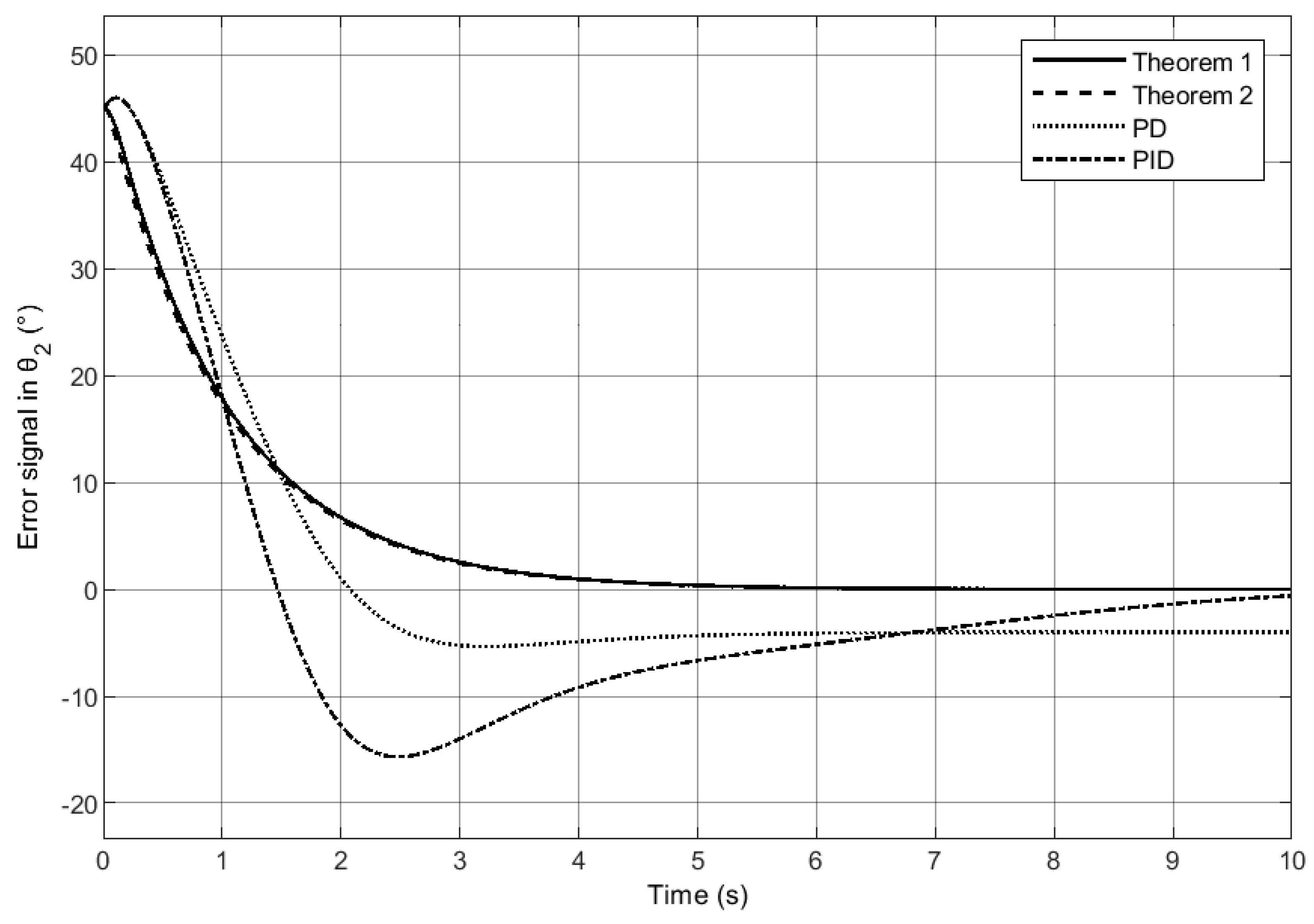
5.2. Two Degrees-of-Freedom Robot

Suppose the two-link manipulator with pivot joints of Figure 3. The link lengths of the manipulator are l 1 and l 2 and the link masses are m 1 and m 2 , with these masses concentrated at the end of each link.
The Hamilton equations of the proposed robot are calculated using Equation (48). Therefore, these equations are written as follows:
p ˙ 1 = τ 1 + G 1 T s 1 + G 2 T s 1 P 1 T s 1 , N 1 1 P 1 P 2 T s 1 , N 1 1 P 1
p ˙ 2 = τ 2 + G 2 T s 2 P 2 T s 2 , N 2 1 P 2
Now, to illustrate the behavior of the previous system with the Theorem 1 is necessary to apply Equation (49). Therefore, the system can be written as:
p ˙ 1 = K 1 s i g n ( S 1 ) + K S 1 S 1 H θ , p , t p 1
p ˙ 2 = K 2 s i g n ( S 2 ) + K S 2 S 2 H θ , p , t p 2
where:
S 1 = θ ˜ 1 + p ˜ 1 S 2 = θ ˜ 2 + p ˜ 2
On the other hand, the behavior of the robot with the Theorem 2 can be written as:
p ˙ 1 = K p 1 θ ˜ 1 + K v 1 p ˜ 1 + p d ˙ 1
p ˙ 2 = K p 2 θ ˜ 2 + K v 2 p ˜ 2 + p d ˙ 2

Comparison

In the same way as the previous example, to simulate the results of the example, it is necessary to implement the parameters in Table 3. However, in this example, the robot has two DoFs. Therefore, the system has two laws of control, where the constant values and equations are chosen as Table 4 (the gains were calculated using [40]). The simulations were performed using Euler’s integration method, with a step size of 0.01 s. The initial conditions were selected as θ 1 ( 0 ) = θ 2 ( 0 ) = 0 , p 1 ( 0 ) = p 2 ( 0 ) = 0 k g m s and the desired values as θ d 1 = 175 , θ d 2 = 45 . Hence, Figure 4 and Figure 5 illustrate the results.
In this example, the efficiency of the algorithm is proved instead of the traditional techniques. The dynamic equations are computed in an iterative form and are easy to develop, which is an advantage for new researchers in the robotic field. On the other hand, in accordance with the simulations, the controllers are faster than the typical laws of control in the industry and they are easy to program in hardware.

6. Conclusions and Future Work

In the present article, the capacity of the proposed method for the modeling and control of robots in phase space is demonstrated. The dynamic equations, in phase space, of an articulated robot can be developed easily and iteratively (which cause it to be easy to program) using the suggested technique. In the examples, it is clearly seen that, with a few simple steps, the equations of motion of the system can be computed; otherwise, when using the traditional method, it is necessary to develop the Euler–Lagrange or Newton–Euler Equations (in addition, the kinematic model should be contemplated before) to later use the Legendre transform; this causes it to be a long and tedious process for new researchers in the field. Talking about the controllers, it is observed how easy it is to build controllers using the screw theory, such as the dynamic equations, where the control laws are obtained iteratively with a few steps. In the simulation, it was shown that the proposed controllers have a better performance than traditional techniques in phase space. Thus, it is illustrated that this technique can be used for the dynamic model and its control in the phase space.
On the other hand, this paper only contemplates the dynamic equations of the robot and its controller. However, the perturbations, unknown parameters, or other external elements are not added to the algorithm. Thus, the previous analysis and the dynamic equations of more complex robots will be taken into account for future work.

Author Contributions

Conceptualization, J.A.M.-H.; data curation, R.L.-P.; formal analysis, A.E.R.-M. and R.L.-P.; funding acquisition, R.B.-A.; investigation, J.A.M.-H.; methodology, J.A.M.-H.; project administration, J.A.M.-H. and R.L.-P.; resources, A.E.R.-M. and R.B.-A.; software, J.A.M.-H. and A.E.R.-M.; supervision, J.A.M.-H. and A.E.R.-M.; validation, R.L.-P. and R.B.-A.; visualization, A.E.R.-M. and R.B.-A.; writing—original draft, J.A.M.-H.; writing—review and editing, J.A.M.-H. and R.L.-P. All authors have read and agreed to the published version of the manuscript.

Funding

This research received no external funding.

Informed Consent Statement

Not applicable.

Data Availability Statement

Not applicable.

Conflicts of Interest

The authors declare no conflict of interest.

Appendix A

Appendix A.1. Robot Dynamics Using Screw Theory

The Lagrangian is written as:
L θ , θ ˙ , t = j = 1 n 1 2 V j T N j V j g ˜ T c ˜ j
Using the Euler–Lagrange equation τ i = d d t L θ , θ ˙ , t θ ˙ i L θ , θ ˙ , t θ i . Hence:
L θ , θ ˙ , t θ ˙ i = j = 1 n 1 2 V j T N j V j g ˜ T c ˜ j θ ˙ i
Here, V j = s j θ ˙ j :
L θ , θ ˙ , t θ ˙ i = j = 1 n 1 2 s j θ ˙ j T N j s j θ ˙ j g ˜ T c ˜ j θ ˙ i
Therefore:
L θ , θ ˙ , t θ ˙ i = j = i n s i T N j V j
Now, differentiating with respect to time:
d d t L θ , θ ˙ , t θ ˙ i = j = i n d d t s i T N j V j
d d t L θ , θ ˙ , t θ ˙ i = j = i n d d t s i T N j V j + s i T d d t N j V j + s i T N j d d t V j
d d t L θ , θ ˙ , t θ ˙ i = j = i n V j T N j a d ( V i ) s i s i T a d T ( V j ) N j V j s i T N j a d ( V j ) V j + s i T N j V j ˙
d d t L θ , θ ˙ , t θ ˙ i = j = i n V j T N j V i , s i + s i T V j , N j V j s i T N j V j , V j + s i T N j V j ˙
where V j , N j V j represent the co-bracket. Considering V 2 , N 2 V 2 T s 1 = V 2 T N 2 s 1 , V 2 :
d d t L θ , θ ˙ , t θ ˙ i = j = i n V ˙ j T N j s i + V j T N j s i , V j + V j T N j V i , s i
On the other hand:
L θ , θ ˙ , t θ i = j = 1 n 1 2 V j T N j V j g ˜ T c ˜ j θ i
L θ , θ ˙ , t θ i = j = 1 n 1 2 V j T θ i N j V j + V j T N j θ i V j + V j T N j V j θ i g ˜ T c ˜ j θ i
L θ , θ ˙ , t θ i = j = i n V j T N j a d ( s i ) V j V i + s i T G j 1 2 V j T a d T ( s i ) N j V j + V j N j a d ( s i ) V j
L θ , θ ˙ , t θ i = j = i n V j T N j s i , V j V i + s i T G j 1 2 V j N j s i , V j V j T s i , N j V j
L θ , θ ˙ , t θ i = j = i n V j T N j s i , V j V i + s i T G j + V j T N j V j , s i
L θ , θ ˙ , t θ i = j = i n G j T s i V j T N j s i , V i
Finally, applying Equations (A9) and (A15) into the Euler–Lagrange equation:
τ i = j = i n V ˙ j T N j s i + V j T N j s i , V j G j T s i

Appendix A.2. Hamilton’s Equations Using Screw Theory

Hamilton’s equation in Equation (44) can be easily computed using Equation (A15). Thus, it can be illustrated by:
H θ , p , t θ i = j = i n P j T s i , N i 1 P i G j T s i
In addition to the foregoing, Hamilton’s equation in Equation (45) can be computed using Equation (A17):
p ˙ i = τ i + j = i n G j T s i P j T s i , N i 1 P i

References

  1. Goldstein, H. Classical Mechanics; Addison-Wesley: Boston, MA, USA, 1980. [Google Scholar]
  2. Taylor, J. Classical Mechanics; G—Reference, Information and Interdisciplinary Subjects Series; University Science Books: Melville, NY, USA, 2005. [Google Scholar]
  3. Peymani, E.; Fossen, T.I. A Lagrangian framework to incorporate positional and velocity constraints to achieve path-following control. In Proceedings of the 2011 50th IEEE Conference on Decision and Control and European Control Conference, Orlando, FL, USA, 12–15 December 2011; pp. 3940–3945. [Google Scholar] [CrossRef]
  4. Arimoto, S. Control Theory of Non-Linear Mechanical Systems: A Passivity-Based and Circuit-Theoretic Approach; Oxford Engineering Science Series; Clarendon Press: Oxford, UK, 1996. [Google Scholar]
  5. Záda, V.; Belda, K. Mathematical modeling of industrial robots based on Hamiltonian mechanics. In Proceedings of the 2016 17th International Carpathian Control Conference (ICCC), High Tatras, Slovakia, 29 May–1 June 2016; pp. 813–818. [Google Scholar] [CrossRef]
  6. Chi, J.; Yu, H.; Yu, J. Hybrid Tracking Control of 2-DOF SCARA Robot via Port-Controlled Hamiltonian and Backstepping. IEEE Access 2018, 6, 17354–17360. [Google Scholar] [CrossRef]
  7. Záda, V. Exponentially stable tracking control in terms of Hamiltonian mechanics. In Proceedings of the 2017 18th International Carpathian Control Conference (ICCC), Sinaia, Romania, 28–31 May 2017; pp. 483–487. [Google Scholar] [CrossRef]
  8. Hestenes, D. Hamiltonian Mechanics with Geometric Calculus. In Proceedings of the Spinors, Twistors, Clifford Algebras and Quantum Deformations; Oziewicz, Z., Jancewicz, B., Borowiec, A., Eds.; Springer: Dordrecht, The Netherlands, 1993; pp. 203–214. [Google Scholar]
  9. Bayro-Corrochano, E.; Zamora-Esquivel, J. Differential and inverse kinematics of robot devices using conformal geometric algebra. Robotica 2007, 25, 43–61. [Google Scholar] [CrossRef]
  10. Dahab, E.A.E. A formulation of Hamiltonian mechanics using geometric algebra. Adv. Appl. Clifford Algebr. 2000, 10, 217–223. [Google Scholar] [CrossRef]
  11. Bayro-Corrochano, E.; Medrano-Hermosillo, J.; Osuna-González, G.; Uriostegui-Legorreta, U. Newton–Euler modeling and Hamiltonians for robot control in the geometric algebra. Robotica 2022, 40, 4031–4055. [Google Scholar] [CrossRef]
  12. Huang, Z.; Li, Q.; Ding, H. Basics of Screw Theory; Springer: Berlin, Germany, 2013; pp. 1–16. [Google Scholar] [CrossRef]
  13. Müller, A. Screw Theory–A forgotten Tool in Multibody Dynamics. PAMM 2017, 17, 809–810. [Google Scholar] [CrossRef] [Green Version]
  14. Ball, R. A Treatise on the Theory of Screws; Cambridge Mathematical Library; Cambridge University Press: Cambridge, UK, 1998. [Google Scholar]
  15. Toscano, G.S.; Simas, H.; Castelan, E.B.; Martins, D. A new kinetostatic model for humanoid robots using screw theory. Robotica 2018, 36, 570–587. [Google Scholar] [CrossRef]
  16. Hunt, K.H. Special configurations of robot-arms via screw theory. Robotica 1986, 4, 171–179. [Google Scholar] [CrossRef]
  17. Selig, J.M. Geometric Fundamentals of Robotics (Monographs in Computer Science); Springer: Berlin/Heidelberg, Germany, 2004. [Google Scholar]
  18. Lynch, K.; Park, F. Modern Robotics: Mechanics, Planning, and Control; Cambridge Univeristy Press: Cambridge, UK, 2017. [Google Scholar]
  19. Yi, B.J.; Kim, W.K. Screw-Based Kinematic Modeling and Geometric Analysis of Planar Mobile Robots. In Proceedings of the 2007 International Conference on Mechatronics and Automation, Harbin, China, 5–8 August 2007; pp. 1734–1739. [Google Scholar] [CrossRef]
  20. Medrano-Hermosillo, J.A.; Lozoya-Ponce, R.; Ramírez-Quintana, J.; Baray-Arana, R. Forward Kinematics Analysis of 6-DoF Articulated Robot using Screw Theory and Geometric Algebra. In Proceedings of the 2022 XXIV Robotics Mexican Congress (COMRob), Mineral de la Reforma/State of Hidalgo, Mexico, 9–11 November 2022; pp. 1–6. [Google Scholar] [CrossRef]
  21. Zou, Y.; Zhang, A.; Zhang, Q.; Zhang, B.; Wu, X.; Qin, T. Design and Experimental Research of 3-RRS Parallel Ankle Rehabilitation Robot. Micromachines 2022, 13, 950. [Google Scholar] [CrossRef] [PubMed]
  22. Sun, T.; Lian, B.; Yang, S.; Song, Y. Kinematic Calibration of Serial and Parallel Robots Based on Finite and Instantaneous Screw Theory. IEEE Trans. Robot. 2020, 36, 816–834. [Google Scholar] [CrossRef]
  23. Liang, Z.; Meng, S.; Changkun, D. Accuracy analysis of SCARA industrial robot based on screw theory. In Proceedings of the 2011 IEEE International Conference on Computer Science and Automation Engineering, Shanghai, China, 10–12 June 2011; Volume 3, pp. 40–46. [Google Scholar] [CrossRef]
  24. Huang, Y.; Liao, Q.; Wei, S.; Guo, L. Research on Dynamics of a Bicycle Robot with Front-Wheel Drive by Using Kane Equations Based on Screw Theory. In Proceedings of the 2010 International Conference on Artificial Intelligence and Computational Intelligence, Sanya, China, 23–24 October 2010; Volume 1, pp. 546–551. [Google Scholar] [CrossRef]
  25. Selig, J.M.; McAree, P.R. Constrained robot dynamics I: Serial robots with end-effector constraints. J. Robot. Syst. 1999, 16, 471–486. [Google Scholar] [CrossRef]
  26. Cheng, J.; Bi, S.; Yuan, C.; Cai, Y.; Yao, Y.; Zhang, L. Dynamic Modeling Method of Multibody System of 6-DOF Robot Based on Screw Theory. Machines 2022, 10, 499. [Google Scholar] [CrossRef]
  27. Qin, Q.; Gao, G. Screw Dynamic Modeling and Novel Composite Error-Based Second-order Sliding Mode Dynamic Control for a Bilaterally Symmetrical Hybrid Robot. Robotica 2021, 39, 1264–1280. [Google Scholar] [CrossRef]
  28. Abaunza, H.; Chandra, R.; Özgür, E.; Ramón, J.A.C.; Mezouar, Y. Kinematic screws and dual quaternion based motion controllers. Control Eng. Pract. 2022, 128, 105325. [Google Scholar] [CrossRef]
  29. Bayro-Corrochano, E. Geometric Algebra Applications Vol. I: Computer Vision, Graphics and Neurocomputing; Springer International Publishing: Berlin/Heidelberg, Germany, 2018. [Google Scholar]
  30. Bayro-Corrochano, E. A Survey on Quaternion Algebra and Geometric Algebra Applications in Engineering and Computer Science 1995–2020. IEEE Access 2021, 9, 104326–104355. [Google Scholar] [CrossRef]
  31. Ji, P.; Li, C.; Ma, F. Sliding Mode Control of Manipulator Based on Improved Reaching Law and Sliding Surface. Mathematics 2022, 10, 1935. [Google Scholar] [CrossRef]
  32. Hestenes, D.; Sobczyk, G. Clifford Algebra to Geometric Calculus: A Unified Language for Mathematics and Physics; Fundamental Theories of Physics; Springer: Dordrecht, The Netherlands, 1987. [Google Scholar]
  33. Perwass, C. Geometric Algebra with Applications in Engineering; Springer: Berlin, Germany, 2009; Volume 4. [Google Scholar] [CrossRef]
  34. Lee, J. Velocity workspace analysis for multiple arm robot systems. Robotica 2001, 19, 581–591. [Google Scholar] [CrossRef]
  35. Siciliano, B.; Sciavicco, L.; Villani, L.; Oriolo, G. Robotics: Modelling, Planning and Control; Advanced Textbooks in Control and Signal Processing; Springer: London, UK, 2010. [Google Scholar]
  36. Craig, J. Introduction to Robotics, Global Edition; Pearson Education Limited: London, UK, 2021. [Google Scholar]
  37. Selig, J.; Ding, X. A screw theory of static beams. In Proceedings of the 2001 IEEE/RSJ International Conference on Intelligent Robots and Systems. Expanding the Societal Role of Robotics in the the Next Millennium (Cat. No.01CH37180), Maui, HI, USA, 29 October–3 November 2001; Volume 1, pp. 312–317. [Google Scholar] [CrossRef] [Green Version]
  38. Utkin, V.I. Sliding Modes in Control and Optimization; Springer Science & Business Media: Berlin/Heidelberg, Germany, 1992. [Google Scholar]
  39. Khalil, H. Nonlinear Systems; Pearson Education; Prentice Hall: Kent, OH, USA, 2002. [Google Scholar]
  40. Kelly, R. A tuning procedure for stable PID control of robot manipulators. Robotica 1995, 13, 141–148. [Google Scholar] [CrossRef]
Figure 1. Single degree-of-freedom robot.
Mathematics 11 00572 g001
Figure 2. Error signals with diverse controllers in θ 1 for a single degree of freedom robot arm.
Mathematics 11 00572 g002
Figure 3. Two-link manipulator.
Mathematics 11 00572 g003
Figure 4. Error signals with diverse controllers in θ 1 for a two degrees-of-freedom robot.
Mathematics 11 00572 g004
Figure 5. Error signals with diverse controllers in θ 2 for a two degrees-of-freedom robot.
Mathematics 11 00572 g005
Table 1. Parameters of the robot.
ParameterValueUnit
m0.25kg
l0.5m
g9.81 m s 2
Table 2. Feedback controllers for the single degree-of-freedom robot.
Law of ControlLaw of ControlGains
Theorem 1See Equation (49) K 1 = 1 , K S 1 = 10
Theorem 2See Equation (55) K p 1 = 25 , K v 1 = 25
PD τ = K p e ( t ) + K v d e ( t ) d t K p = 25 , K v = 25
PID τ = K p e ( t ) + K I e ( t ) d t + K v d e ( t ) d t K p = 25 , K I = 15 , K v = 25
Table 3. Parameters of the robot.
ParameterValueUnit
m 1 , m 2 0.25kg
l 1 , l 2 2m
g9.81 m s 2
Table 4. Feedback controllers.
Law of ControlLaw of ControlGains
Theorem 1See Equation (49) K 1 = K 2 = 1 ; K S 1 = K S 2 = 10
Theorem 2See Equation (55) K p 1 = K p 2 = 25 ; K v 1 = K v 2 = 25
PD τ = K p e ( t ) + K v d e ( t ) d t K p = K v = 25 0 0 25
PID τ = K p e ( t ) + K I e ( t ) d t + K v d e ( t ) d t K p = K v = 25 0 0 25 , K I = 15 0 0 15
Disclaimer/Publisher’s Note: The statements, opinions and data contained in all publications are solely those of the individual author(s) and contributor(s) and not of MDPI and/or the editor(s). MDPI and/or the editor(s) disclaim responsibility for any injury to people or property resulting from any ideas, methods, instructions or products referred to in the content.

