Abstract
Shared bicycles provide a green, environmentally friendly, and healthy mode of transportation that effectively addresses the “final mile” problem in urban travel. However, the uneven distribution of bicycles and the imbalance of user demand can significantly impact user experience and bicycle usage efficiency, which makes it necessary to predict bicycle demand. In this paper, we propose a novel shared-bicycle demand prediction method based on station clustering. First, to address the challenge of capturing patterns in station-level bicycle demand, which exhibits significant fluctuations, we employ a clustering method that combines graph information from the bicycle transfer graph and potential energy. This method aggregates closely related stations into corresponding prediction regions. Second, we use the GCN-CRU-AM (Graph Convolutional Network-Gated Recurrent Unit-Attention Mechanism) model to predict bicycle demand in each region. This model extracts the spatial information and correlation between regions, integrates time feature data and local weather data, and assigns weights to the input features. Finally, experimental results based on the data from Citi Bike System in New York City demonstrate that the proposed model achieves a more accurate demand prediction.
MSC:
68T07; 90B20
1. Introduction
With the accelerated process of urbanization and the escalating problem of traffic congestion, shared bicycles have experienced rapid growth as a green, low-carbon, and convenient mode of transportation. According to statistical data, as of 2021, the global market size of shared bicycles has exceeded 15 billion USD and is expected to reach 30 billion USD by 2025 [1]. However, in many cities, there are significant spatial and temporal variations in the distribution and demand for shared bicycles [2]. Without predicting the occurrence of bicycle shortages and surpluses in advance, these variations can result in underutilized shared-bicycle resources and inadequate supply in certain areas. Therefore, predicting the user demand in shared-bicycle systems plays a crucial role in promoting the intelligent and sustainable development of urban transportation.
Shared-bicycle demand prediction refers to the process of forecasting the demand for shared bicycles during a specific future time period through the analysis and modeling of historical data. Currently, shared-bicycle demand prediction methods can be broadly categorized into two types.
The first type is station-level methods, in which each individual shared-bicycle station is considered as the basic prediction unit, and the demand for bicycles within each station is predicted separately. Huang et al. [3] proposed a Bimodal Gaussian Inhomogeneous Poisson (BGIP) algorithm for predicting the number of bicycles at each station. Chen et al. [4] developed a model based on recurrent neural networks (RNN) to predict the real-time rental and return demand at each bicycle station, which can be used to formulate load-balancing strategies between stations. Zi et al. [5] introduced the TAGCN (Temporal Attention Graph Convolution Network) model, which combines graph convolutional neural networks with attention mechanisms to address the problem of the bike check-out/in number prediction of each station.
The other method category is based on cluster-level analysis. Due to the fact that the usage patterns of bicycles at each station are susceptible to factors such as time and weather, it is challenging to predict the demand for shared bicycles at individual stations. Algorithms of this type group similar stations into the same cluster and predict the demand for bicycles within each cluster.
Feng et al. [6] proposed a hierarchical traffic prediction model that utilizes iterative spectral clustering to cluster stations and employs a gradient boosting regression tree to predict the rental count for the entire shared-bicycle system. Jia et al. [7] proposed a two-stage Gaussian mixture model (GMM) clustering algorithm for shared bicycle stations, which considers bicycle migration trends and geographic location information between stations. Hua et al. [8] divided the virtual stations of dockless bike-sharing through K-means clustering and used random forest to predict the demand. Chen et al. [9] introduced a cluster-based dynamic prediction algorithm that constructed a weighted relationship network based on the current environment to simulate the relationships between bicycle stations. Stations with similar usage patterns are dynamically grouped into clusters.
Table 1 summarizes the differences between these two types of methods for predicting shared-bicycles demand and demonstrates whether the features are considered in each study.

Table 1.
Two types of shared-bicycle demand prediction methods considering different features.
Through the analysis of Table 1 and the current research status, its limitations are as follows:
- Most studies do not consider the connection between shared-bicycle stations. Simply studying the demand of a single station is not enough to improve the service quality of the entire city’s shared bicycle system.
- Previous studies primarily utilized the bipartite clustering model (BC) [10], the unified geographic grid clustering (GC) algorithm, and K-means [9] to cluster bike stations. These methods have disadvantages such as not considering the migration trend of shared bikes between stations and relying heavily on randomly initialized parameters [11].
- Some existing demand prediction models use traditional machine learning methods, such as random forest [9,12], support vector machine [13], linear regression [14], gradient boosting regression tree [6,8], etc. These models have shortcomings such as difficulty in handing complex relationships, limitations in feature interactions, and limited ability to model time series in the prediction of shared-bicycle demand. Additionally, some deep learning methods [5,15] used for demand prediction have limitations in terms of incomplete consideration and insufficient prediction. Specifically, these methods only take into account two aspects of spatial, temporal, or weather features, neglecting the holistic nature of the problem.
In order to overcome the deficiencies of existing bicycle demand prediction methods, this paper provides a novel shared-bicycle demand prediction method based on GIPE (Graph Information and Potential Energy) clustering and the GCN–GRU–AM (Graph Convolutional Network–Gated Recurrent Unit–Attention Mechanism) deep neural network. Its main contributions include the following:
- We construct a bicycle transfer graph that considers the migration trend of shared bicycles between stations and extract graph information by calculating the importance degree of each station. Making full use of the graph information can effectively improve the clustering accuracy of shared-bicycle stations.
- We apply the idea of potential energy to the correlation between stations, so that stations with more similar bicycle usage patterns and more frequent circulation can be reasonably clustered into the same regions.
- In addition to historical bicycle demand features, we also consider the impact of weather features and time features on shared-bicycle demand prediction and evaluate different features through experiments.
- Based on the deep neural network, we construct a GCN–GRU–AM model to predict the demand for shared bicycles, which can capture the spatial correlation between regions and the long-term and short-term dependencies in time series data and assign weights to different features. The experimental results show that the model’s prediction accuracy is better than that of other models.
The rest of the paper is organized as follows: In Section 2, we provide a comprehensive description of our station clustering method and the shared-bicycle demand prediction model, offering detailed insights into their methodologies and techniques. In Section 3, we present the experimental process, including a comparative analysis of our approach with other models, as well as an exploration of the different feature inputs and various clustering methods. In Section 4, we outline the findings and conclusions of this study, providing a comprehensive summary and highlighting the implications of our research.
2. Materials and Methods
In this section, we present the methods proposed in this paper, which contain the station clustering method and the demand prediction model.
2.1. Station Clustering Method
The usage of bicycles in a shared-bicycle system is influenced by multiple factors such as the bicycle’s time of use, weather conditions, and the unique relationships between stations [16]. This implies that the demand for bicycles varies significantly depending on these conditions, which makes it difficult to capture its regularity and predictability. By aggregating stations with similar characteristics, the accuracy of demand prediction can be improved, especially when compared to analyzing individual stations. Additionally, the users’ riding habits are not limited to one station, so when users cannot find bicycles at their current station, they will go to nearby stations to search for bicycles. When users want to return their bicycles but find that the parking spots are full, they may also go to nearby stations to park their bicycles. Therefore, the proximity between stations has some correlation from the users’ perspective [6].
In this section, we propose a clustering method based on graph information and potential energy to solve the problem of inter-station correlations.
2.1.1. Graph Information
- Bicycle Transfer Graph;The bicycle transfer between shared-bicycle stations is essentially similar to the strong and weak associations between nodes in a graph. The correlation between different bicycle stations can also be represented by a graph. We define a bicycle transfer graph as a weighted directed network , in which the nodes represent the set of single stations , the lines with arrows represent the set of edges , and the means represents the transfer quantity from station to station . The bicycle transfer relationship between nodes is shown in Figure 1, which is a schematic diagram.
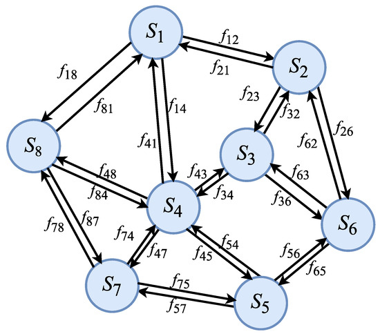 Figure 1. Bicycle transfer graph.
 - Station Importance Degree Matrix;The initial importance degree matrix for each station is defined as the proportion of bicycle usage at each station to the bicycle usage at all stations in a certain time period. Assuming there are nodes in the bicycle transfer graph and that the total bicycle usage in this period is , the bicycle usage of station is ; the calculation formula for the initial importance matrix is shown as follows:
- Adjacency Matrix;The adjacency matrix represents the bicycle flow between each station.We calculate the number of bicycles that can be transferred from one station to another and the total number of bicycles that can be reached from other stations to the current station to construct the bicycle transfer matrix and the station bicycle arrival volume matrix . The calculation method for the adjacency matrix is as follows:represents the number of bicycle transfer from station to station in a certain period, and represents the total number of bicycles arriving at station within a certain period.
The importance degree of each station is calculated from the above adjacency matrix and the initial station importance degree matrix . The specific calculation process is as follows:
In the above equations, is a parameter between 0 and 1 that determines the relative importance of the station’s borrowing behavior and the bicycle flow behavior between stations. In the final station importance degree matrix, represents the station importance degree obtained by the user’s bicycle usage behavior at station , and represents the circulation importance degree feedback from station ’s user bicycle usage importance degree to site due to the bicycle flow between station and station . Similar to graph nodes, the importance degree of each node in the graph is not only related to itself but also affected by the nodes with which it is connected.
By extracting the graph information from the bicycle transfer graph through the above calculation process, the final station importance degree is obtained from the node importance degree matrix, in which , indicating the importance degree of station in the bicycle transfer graph.
2.1.2. Potential Energy between Stations
The correlation between bicycle stations is determined by the distance between stations and the overall importance of each station in the bicycle network. The mutual influence between stations can be compared to the attraction between different planets, where stations with higher importance have a larger range and capability of influence. Comparing the complex bicycle network to a large galaxy, the clustering process is equivalent to distinguishing small galaxies with strong correlations, such as the solar system in which the Earth is located. Referring to the universal gravitational formula between planets, the potential energy between station and station is calculated as follows:
and represent the importance of stations and , represents the distance between two stations, and represents the corresponding distance influence factor, which is a customizable parameter used to adjust the degree of influence caused by distance between stations.
2.1.3. Station Clustering Method
The main idea of the clustering method in this paper is based on the importance degree and correlation between the stations in the bicycle station network. The goal of the clustering method is to select the most important and closely related stations from the bicycle transfer graph and then classify them into clusters based on their distance from the cluster center. In addition, each cluster only contains stations that have a maximum potential energy with the current cluster center.
The main process of the clustering method is as follows:
- Extract station information from the bicycle order data and construct the bicycle transfer graph;
- Extract graph information by calculating the importance degree and nearest-neighbor distance with high-importance degrees for all stations by using the bicycle transfer graph;
- Construct a decision diagram based on station importance degrees and nearest neighbor distance with high-importance degrees. Based on this diagram, nodes with higher importance degrees and high-importance degree nearest-neighbor distances are selected as cluster centers; and
- Classify the remaining nodes according to their potential energy with the cluster center based on the principle of maximizing potential energy.
Figure 2 illustrates the clustering process of the proposed method.
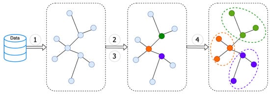
Figure 2.
Process of the GIPE clustering method.
The core steps of the GIPE clustering method include calculating the importance of stations in the bicycle transfer graph and allocating the remaining stations based on their potential energy. The specific allocation process of the remaining stations after selecting the cluster centers is shown in Figure 3.
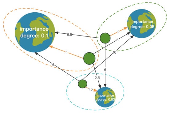
Figure 3.
Station allocation of the GIPE clustering method.
In the station allocation diagram, there are three cluster centers with importance degrees of 0.1, 0.05, and 0.03, respectively. These three green circles represent the stations to be allocated. The values on the arrows represent the potential energy between the current station to be allocated and the cluster center, and the orange line indicates the final allocation result of the station. Through the station allocation process, it can be seen that the degree of association between stations not only depends on their importance but also relates to the distance between different stations. The cluster centers with higher importance and closer distance to the current station are more attractive, and the mutual circulation of bicycles between them is also more frequent.
2.2. Demand Prediction Model
This paper proposes a deep learning model for bicycle demand prediction. The input features include historical bicycle demand data in various regions, time-related feature data, and corresponding weather feature data at the same time. Firstly, the GCN is employed to capture spatial correlations, and then a multi-layer GRU is designed to learn the associations between time series. Additionally, an attention mechanism is adopted to extract historical time step data information and inter-regional features with different weights, enabling the final model to have a good ability to predict demand. Finally, the dense layer outputs the bicycle demand in each time period for the 26 clustered regions. The model includes the input layer, the GCN layer, the GRU layer, the attention layer, and the output layer, as shown in Figure 4 [17].
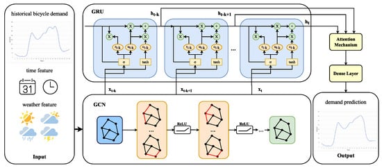
Figure 4.
The structure of the GCN–CRU–AM model.
- Input Layer:This layer is used to receive bicycle demand, time features, and weather features. The data form can be expressed as , in which , represents the time length of the input sequence, represents the feature dimension of the input data, and represents the feature vector at time . In this paper, the value of is 32, including bicycle demand in 26 areas, three-dimensional time features and three-dimensional weather features.
- GCN Layer [18]:This layer used to capture the spatial correlation between regions. First, we construct a region adjacency matrix to represent the connection relationship between regions. Assuming that there are bicycle station regions, the amount of bicycle transfers from region to region in a certain period is , and the total number of bicycles arriving in region during this period is , then the adjacency matrix between regions can be expressed as follows:The adjacency matrix is a matrix, where represents the connection strength between region to region , which can be expressed as = . The original adjacency matrix is normalized to obtain the matrix :The basic operation of the GCN can be expressed as:Here, is the normalized adjacency matrix, is the feature representation of the -th layer, is the weight matrix of the -th layer, and is the activation function (such as ReLU). We applied multiple GCN layers to extract spatial features. The GCN operation of each layer will update the node features in order to capture the higher-order spatial correlations [19].
- GRU Layer [20]:This layer is used to capture long -short-term dependencies in time series data. This module receives feature sequences from the GCN module and processes them in sequence over time, capturing temporal features in the input sequence, such as trends and periodicity. The GRU utilizes gate structures to control the generation and forgetting of information. Meanwhile, it also uses the state of the previous moment to calculate the state of the current moment, thereby achieving the modeling of sequence historical data and long-term memory [21].We used a fully connected layer to fuse the spatial features extracted by the GCN layer with other input features (weather features and time features). Next, we employed multiple GRU units to model the fused features, with each GRU layer containing 128 hidden neurons and using sigmoid activation functions to learn the time series relationships between data. The hidden layer output serves as the input for the subsequent attention mechanism layer. The gated structure of the GRU can effectively handle dependencies at different time scales, thereby capturing the temporal dynamics of bicycle demand.In Figure 4, represents the output of the GCN layer when the input data at time is provided to it, and denotes the hidden layer output of the GRU layer after memorizing and forgetting the current input and the historical information. Ultimately, these are passed to the attention mechanism layer to assign weights from different inputs.
- Attention Layer:This layer is used to address the issues of information loss and the vanishing gradient encountered by the GRU layer when handling long sequences. This mechanism computes the feature weights for the hidden layer in the GRU, which can preserve important features and reduce the impact of interference information. In this paper, we adopt the additive attention mechanism and the specific calculation process is as follows:is used to calculate the similarity score between and , where represents vector splicing and is an activation function. Additionally is the normalized attention weight.
- Output LayerThis fully connected layer is used to map the attention-weighted GRU output to the predicted bicycle demand, that is, the future bicycle demand in 26 regions. Assuming that the output is , the calculation process of the output layer is:and are the weight matrix and bias of the output layer, respectively.
3. Results and Discussion
3.1. Experimental Datasets
3.1.1. Shared Bicycle Data
This study utilizes a publicly available dataset from Citi Bike in New York City for research purposes [22]. The dataset consists of 6.14 million bicycle ride order records from July to August 2021, obtained from the official Citi Bike website. Table 2 presents a partial overview of the raw data fields collected for Citi Bike orders in this study.
Table 2.
Citi Bike order data.
3.1.2. Weather Data
This study collected hourly weather report data for New York City from July to August 2021 to complement the analyzed Citi Bike dataset [23,24]. The weather report data from Weather Underground includes hourly reports for various weather parameters in New York City during this period. The report format consists of timestamps, wet bulb temperatures, dry bulb temperatures, humidity, pressure, and wind speeds. It should be noted that the original data may contain missing values for wind speed and humidity. To ensure the continuity of the meteorological data, this study employs a method for filling in the missing values using the previous hour’s weather report data.
3.2. Result of Clustering
From the original bicycle order data, this study extracted 1451 station records. To ensure the reasonability of the research, a rectangular division approach was adopted. Stations within the longitude range of 40.68° N to 40.77° N and the latitude range of −74.02° W to −73.95° W were selected. A total of 487 stations were filtered for subsequent experimental research. For extracting station graph information and calculating inter-station potential energy, data from five consecutive working days were selected. Figure 5 illustrates the selected research stations and the clustering results of the stations using the graph information and potential energy clustering method.
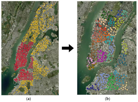
Figure 5.
Regional site screening and clustering results: (a) station filter, and (b) clustering results.
The clustering results from Figure 5 reveal that the centers of each clustered region are reasonably spaced, with no closely located cluster centers. Furthermore, the number and distribution of stations within each cluster region are relatively even. These observations indicate that the clustering algorithm effectively selected appropriate cluster centers and achieved a satisfactory division of stations. The clustering results align well with the actual distribution of the stations.
From the comparison of the clustering results in Figure 6, it is evident that the K-means algorithm [25] can relatively evenly aggregate stations in different regions. However, it tends to overlook the influence of actual geographical factors and local residents’ travel habits. The clustering results do not align with the actual distribution of user demand, which may result in the aggregation of unrelated stations. As a result, the demand for station clusters fluctuates significantly, impacting the model’s ability to predict the demand for different cluster groups.
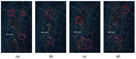
Figure 6.
Comparison of the results of the four clustering methods: (a) K-means, (b) DBSCAN, (c) DPC, and (d) GIPE.
DBSCAN [26], on the other hand, performs station clustering by setting the minimum number of points in each cluster and the corresponding search radius. However, the stations in this study were extracted from the bicycle order data, and the actual stations are fixed stations with their locations determined by the bike-sharing operator. The station distribution is relatively uniform, and density clustering does not effectively capture the actual correlations between stations. Additionally, determining the number of clusters is challenging, and the sizes of the clusters vary significantly, deviating from the actual rules for dividing stations into regions.
DPC clustering [27], as a density peak-based algorithm, has similar reference metrics to DBSCAN but has different rules for assigning the remaining points. DPC clustering is better able to specify the number of cluster regions, select high-density stations as cluster centers, and divide the remaining stations based on density and distance correlations. However, similar to DBSCAN, DPC clustering also exhibits significant differences in cluster sizes. Some clusters become excessively large, which hinders accurate bicycle predictions between regions.
The GIPE clustering method proposed in this study, which combines graph information and potential energy, not only evaluates the importance degree of each station in the bicycle transfer graph from the perspective of actual demand but also selects distant stations with high-importance degrees as cluster centers. Additionally, it utilizes potential theory to calculate the attractiveness of each cluster center to the remaining stations, representing the degree of correlation between stations. This approach enables the final clustering of stations. The clustering results align well with reality, and the distribution of the stations within each cluster is relatively even, meeting the basic requirements of regional prediction and bicycle scheduling research.
3.3. Result of Demand Prediction
3.3.1. Baseline Method
The problem of demand prediction in the different regions and time periods of shared bicycles, can essentially be formulated as a time series forecasting task. Various deep models are commonly used to address such problems. In this study, the GCN–GRU–AM model is employed, and its performance is evaluated by comparing it with several benchmark methods from existing research or state-of-the-art approaches.
- CNN [28]: The convolutional neural network (CNN) model is a typical model for extracting spatial information from data. It can also be applied to bicycle demand prediction tasks by extracting useful information from the raw bicycle demand data and weather data, enabling effective prediction of future bicycle demand.
- LSTM [29]: As a variant of the recurrent neural network (RNN), the long short-term memory (LSTM) is one of the most commonly used deep models for handling time series forecasting problems and has been widely applied in various research studies.
- GRU [21]: GRU is similar to LSTM but has a simpler internal structure. It discards the complex cell state and uses only the memory gate and the forget gate to achieve a similar functionality to LSTM. GRU has fewer parameters and is simpler to train.
- XGBoost [30]: XGBoost is a model that employs decision trees for prediction or classification tasks. Compared to traditional random forest models, XGBoost demonstrates superior performance, wider applicability, and a significantly improved training speed.
- GCN [31]: The GCN combines graph theory with CNN by constructing a reasonable graph relationship (adjacency matrix) for node-type data. It effectively captures spatial information between nodes and achieves significant performance improvement by integrating with the CNN module.
- GRU-AM [32]: GRU–AM is a hybrid model, in which the GRU structure is first used to preserve historical information, and then the temporal attention mechanism (AM) is used to give different weights to the features.
- CNN-GRU [33]: The CNN–GRU model is a fusion deep-learning approach that combines a convolution neural network (CNN) and gated recurrent units (GRUs).
- CNN–GRU–AM [34]: The CNN–GRU–AM model is a combination of three different techniques. First, CNN is used to extract local features from the data. Second, GRU is employed to capture the time-series relationships of the output data of CNN. Finally, the AM is introduced to mine the potential relationships of the series features.
- T-GCN [19]: The temporal graph convolutional network (T–GCN) model is combined with the GCN and GRU to capture the spatial and temporal dependences simultaneously.
3.3.2. Evaluation Indicators
- Mean Absolute Error (MAE):
- Root Mean Square Error (RMSE):
- Root Mean Squared Logarithmic Error (RMSLE) is a metric commonly used to evaluate the performances of different models on the same research problem across different datasets. It measures the relative error and is defined as follows:
In this equation, represents the actual value, and represents the model predicted value.
MAE and RMSE are used to evaluate the deviation between model prediction results and actual demand, that is, the absolute error, while RMSLE is used to evaluate the deviation between model prediction results and actual demand, reflecting the model’s ability to predict the overall change trend.
3.3.3. Experimental Setup
When considering the demand prediction problem, it is necessary to identify the data characteristics of the main objective and subjective factors related to bicycle demand and assess the importance of different features. In this study, demand-related features, time features, peak-hour features, and weather features, which are closely related to bicycle demand prediction, were selected. XGBoost was used to evaluate the different features.
According to the feature analysis results in Figure 7, it is evident that the original demand sequence is crucial for model training. Hourly information, morning and evening peak indicators (represented by 1 and 2, respectively), and the weekday attribute (ranging from 1 to 7) also exhibit significant effects. On the other hand, weather features have a relatively smaller impact as compared to other features. However, they still contribute to improving the model’s demand prediction performance. In this study, selected weather features include temperature, humidity, and wind speed.
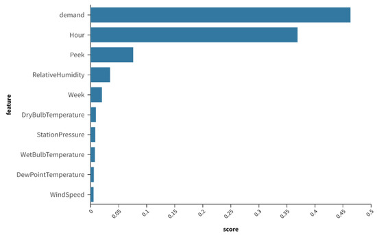
Figure 7.
Feature importance degree analysis.
The impact of the time step on the prediction performance of the basic GRU model was investigated. The most appropriate time step was selected and used as the “time_step” parameter for all of the deep models. The input features for the GRU model consist of the combination of bicycle demand, time features, and weather features. Experimental results for the different regions’ bicycle demand predictions using the GRU model under different time steps are presented in Table 3.
Table 3.
Performance of the GRU model at different time steps.
From the experiment results in Table 3, it can be observed that the demand prediction performance of the GRU model shows an overall trend of first increasing and then weakening with the time steps. Normally, considering that the station status in the previous time period affects the station status in the current time period, the accuracy of the prediction is higher with the larger time step. However, when the time step reaches a certain value, due to the addition of noise features that are irrelevant to time series prediction, the prediction performance does not increase but rather decreases, and the training time is increased. Therefore, the time step is selected to be four through the experiments. At this time, the RMSE, MAE, and RMSLE of the GRU model are all minimum values.
3.3.4. Performance Analysis
- Performance Analysis of the GCN–CRU–AM model
Based on the station-clustering results, we compared the performance of different deep learning models in predicting the actual bicycle demand under the same input data features. The input features include historical demand, time, and weather characteristics. We used the data of 34 consecutive working days as the training and validation set, and the subsequent nine working days as the test set. Each model is trained for 100 epochs, and the demand prediction results are calculated by subtracting the actual demand. The multiple error values are obtained and statistically analyzed, as shown in Table 4.
Table 4.
Comparison of the demand prediction performances of different deep learning models.
From the experimental data presented in Table 4, it can be observed that among the various deep learning models, the GCN–GRU–AM model adopted in this study exhibits a good demand prediction performance. The RMSLE of predicting check-out demand in various regions reaches 0.335, and the RMSE is 15.291. For check-in demand, the RMSLE and RMSE are 0.331 and 14.905, respectively. These figures are significantly lower than those of other models, indicating that the GCN–GRU–AM model has a strong capability for predicting the future demands for shared bicycles in each region.
Among the remaining models, the basic LSTM performs worst, and the GRU shows a certain degree of performance improvement over LSTM. Compared to the LSTM and GRU models, XGBoost has smaller demand prediction error values, indicating that its basic performance is superior to the LSTM and GRU in the context of this study. After incorporating the Attention Mechanism into the GRU model, its RMSE, MAE, and RMSLE errors decrease, suggesting that the combination of the attention mechanism and the GRU module enhances the model’s predicting performance.
The performance of the original GCN model is better than that of LSTM and GRU models but is somewhat inferior to XGBoost. Although the GCN extracts information from different regional demand and other features, it lacks a time-series learning module, which may cause the temporal information to be overlooked and hinder the learning of associativity between time series. By incorporating the GRU module to effectively extract input information, the model performance improves significantly, with the RMSLE, RMSE, and MAE slightly better than those of the CNN–GRU–AM model, which exhibits the best performance among the remaining models.
To intuitively demonstrate the effectiveness of the GRU module and the attention mechanism module in the GCN model, the check-out demand prediction results of the 2nd clustering region from the GCN, GCN–GRU, and GCN–GRU–AM models are compared with the actual check-out demand. This comparison aims to investigate the influence of the different modules on the final model performance.
By comparing the demand prediction results of the GCN, GCN–GRU, and GCN–GRU–AM models with the actual demand prediction results in Figure 8, it can be observed that the prediction results of the GCN model have the lowest fitting degree with the actual demand. The demand prediction results during the morning and evening rush hours are relatively accurate, while the prediction deviation of bicycle demand during lunchtime is relatively large. With the addition of the GRU model, the prediction performance of bicycle demand during the day improves. On this basis, the GCN–GRU–AM model, which incorporates the attention mechanism, enhances the prediction accuracy during the morning and evening rush hours and lunchtime, thereby improving the overall performance of the model.
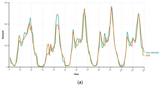
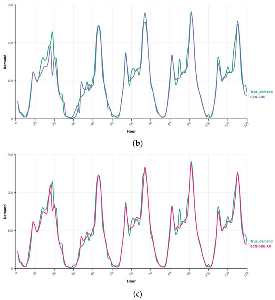
Figure 8.
Comparison of the prediction result with the actual demand in Region 2. (a) Comparison of the GCN prediction results with the actual demand in Region 2, (b) Comparison of the GCN–GRU prediction result with actual demand in Region 2, and (c) Comparison of the GCNGRU–AM prediction result with actual demand in Region 2.
In order to present the demand prediction performance of different models more intuitively, Figure 9 shows the check-in demand prediction results of the different models compared with the actual demand data in Region 22 for four consecutive working days, from 22 to 25 August 2021. We compared the GCN–GRU–AM model with the XGBoost model, which preforms better in the basic models, and the CNN–GRU–AM model, which has a better performance among the hybrid models.
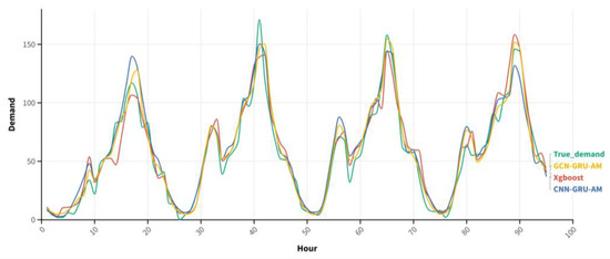
Figure 9.
Prediction results of the different models over multiple working days.
It can be seen from Figure 9 that each model has a certain deviation from the original demand when making actual predictions of working-day demand. Among them, the model with a larger error index has a larger performance deviation in actual prediction. The GCN–GRU–AM model used in this article hac the best performance and has a high degree of fit with the original demand curve.
- 2.
- The Impact of Input Features on Model Performance
For deep learning models, their performance not only depends on their structure but also on the quality of the input data and the feature dimension, which greatly affect the final performance of the model. Using the GCN–GRU–AM model, we conducted experiments by combining the different input data features to test the impact of the various features on the model’s demand prediction performance. The specific experimental data is presented in Table 5.
Table 5.
Analysis of model demand prediction performances with different feature combinations.
In the comparison of model performance under different features, the GCN–GRU–AM model trained with the input data of the demand in different regions and time periods performs worst. By adding time-based and weather features for model training, the demand prediction performance improves. Among them, the model trained with time-based features performed better than the model trained with weather features, indicating that time-based feature data contributes more to the improvement of the model performance than the weather features. This is consistent with the results of the analysis using the XGBoost model to assess the different features in Section 3.3.3. By combining time-based and weather features, the demand prediction error rate of the model further decreases. The input feature data used in the final demand forecasting model of this paper includes the combination of demand data, time-based feature data, and weather feature data.
- 3.
- Effectiveness Analysis of Clustering Method
To validate the effectiveness of the proposed GIPE clustering method, we perform clustering on the initial 577 stations using other clustering methods. Combining the clustering results with the calculated demand for each clustering region and time period, we obtained the demand data under different clustering methods. Then, we trained the GCN–CRU–AM model using the demand data estimated by the different clustering methods and predicted the future demand in each region. This enabled us to assess the model’s performance under various clustering methods. In addition, K-means and DPC clustering methods generate 26 clusters, the same as the GIPE clustering method. Because the DBSCAN clustering algorithm has an uncertain number of clusters, it is not included in the comparison among the different clustering methods.
After re-constructing the adjacent matrix and re-statistically calculating the historical demand for each region, the GCN–GRU–AM model is trained for the future demand prediction of each region based on the clustering results from different clustering methods. Table 6 summarizes the experimental performance data of the GCN–GRU–AM model trained using the clustering results of different clustering methods.
Table 6.
Performance analysis of demand forecasting models with different clustering methods.
Compared with the K-means clustering method that only considers node distance and the DPC clustering method that only considers node density and distance, the clustering method in this paper considers the actual bicycle usage and distance factors. In this case, the bicycle demand forecast error value is smaller thanks to the use of the same GCN-GRU-AM model for training.
4. Conclusions
Shared bicycle systems are an important part of urban public transportation, and demand prediction can improve resource allocation, optimize bicycles management, and enhance user experience. Furthermore, our research on this subject can support policy-makers in making informed decisions and formulating effective strategies, such as optimizing the distribution of shared bicycles across different regions, planning for infrastructure development, and designing targeted promotional campaigns to encourage bicycle usage.
In this paper, we propose a novel shared-bicycle demand prediction model based on station clustering. Taking into consideration the user’s riding habits and the correlation between the different stations in the actual shared-bicycle system, we constructed a bicycle transfer graph based on bicycle trip data and cluster stations by calculating each station’s importance degree and the inter-station potential energy. In the demand prediction problem, we consider time features and weather features that affect the demand for shared bicycles and incorporate them as key features into the GCN-GRU-AM model constructed in this paper for analyzing the shared-bicycle demand within clusters during different time periods. The experimental results demonstrate that the proposed demand prediction model has a high degree of alignment with the actual bicycle demand data and can effectively predict the bicycle demand in different regions and time periods, thereby outperforming other models in terms of performance.
In future works, we will utilize annual data for research and incorporate seasonal features into the deep-model training to enhance the model’s versatility. Moreover, because the current method to solve the imbalance of bicycle demand within stations is manual dispatch, future research will seek optimal inter-station paths in order to reduce the cost of manual dispatch.
Author Contributions
Conceptualization, J.-Y.X. and Y.Q.; methodology, Y.Q. and C.-C.W.; software, Y.Q. and S.Z.; validation, J.-Y.X. and Y.Q.; formal analysis, C.-C.W. and J.-Y.X.; investigation, Y.Q.; resources, J.-Y.X.; data curation, Y.Q. and J.-Y.X.; writing—original draft preparation, S.Z. and Y.Q.; writing—review and editing, J.-Y.X., C.-C.W. and Y.Q.; visualization, S.Z.; supervision, J.-Y.X.; project administration, J.-Y.X.; funding acquisition, J.-Y.X. All authors have read and agreed to the published version of the manuscript.
Funding
This work was supported in part by the National Natural Science Foundation of China grant number 72271048, and by the National Science and Technology Council of Taiwan, NSTC 112-2221-E-035-060-MY2.
Data Availability Statement
The corresponding author will provide the relative datasets upon request.
Conflicts of Interest
The authors declare no conflict of interest.
References
- Zheng, L.; Li, Y. The Development, Characteristics and Impact of Bike Sharing Systems. Int. Rev. Spat. Plan. Sustain. Dev. 2020, 8, 37–52. [Google Scholar] [CrossRef] [PubMed]
- Li, Y.; Zheng, Y. Citywide Bike Usage Prediction in a Bike-Sharing System. IEEE Trans. Knowl. Data Eng. 2020, 32, 1079–1091. [Google Scholar] [CrossRef]
- Huang, F.; Qiao, S.; Peng, J.; Guo, B. A Bimodal Gaussian Inhomogeneous Poisson Algorithm for Bike Number Prediction in a Bike-Sharing System. IEEE Trans. Intell. Transp. Syst. 2019, 20, 2848–2857. [Google Scholar] [CrossRef]
- Chen, P.-C.; Hsieh, H.-Y.; Sigalingging, X.K.; Chen, Y.-R.; Leu, J.-S. Prediction of Station Level Demand in a Bike Sharing System Using Recurrent Neural Networks. In Proceedings of the 2017 IEEE 85th Vehicular Technology Conference (VTC Spring), Sydney, NSW, Australia, 4–7 June 2017; pp. 1–4. [Google Scholar] [CrossRef]
- Zi, W.; Xiong, W.; Chen, H.; Chen, L. TAGCN: Station-Level Demand Prediction for Bike-Sharing System via a Temporal Attention Graph Convolution Network. Inf. Sci. 2021, 561, 274–285. [Google Scholar] [CrossRef]
- Feng, S.; Chen, H.; Du, C.; Li, J.; Jing, N. A Hierarchical Demand Prediction Method with Station Clustering for Bike Sharing System. In Proceedings of the 2018 IEEE Third International Conference on Data Science in Cyberspace (DSC), Guangzhou, China, 18–21 June 2018; pp. 829–836. [Google Scholar] [CrossRef]
- Jia, W.; Tan, Y.; Liu, L.; Li, J.; Zhang, H.; Zhao, K. Hierarchical Prediction Based on Two-Level Gaussian Mixture Model Clustering for Bike-Sharing System. Knowl.-Based Syst. 2019, 178, 84–97. [Google Scholar] [CrossRef]
- Hua, M.; Chen, J.; Chen, X.; Gan, Z.; Wang, P.; Zhao, D. Forecasting Usage and Bike Distribution of Dockless Bike-Sharing Using Journey Data. IET Intell. Transp. Syst. 2020, 14, 1647–1656. [Google Scholar] [CrossRef]
- Chen, L.; Zhang, D.; Wang, L.; Yang, D.; Ma, X.; Li, S.; Wu, Z.; Pan, G.; Nguyen, T.-M.-T.; Jakubowicz, J. Dynamic Cluster-Based over-Demand Prediction in Bike Sharing Systems. In Proceedings of the 2016 ACM International Joint Conference on Pervasive and Ubiquitous Computing, Heidelberg, Germany, 12–16 September 2016; pp. 841–852. [Google Scholar] [CrossRef]
- Li, Y.; Zheng, Y.; Zhang, H.; Chen, L. Traffic Prediction in a Bike-Sharing System. In Proceedings of the 23rd SIGSPATIAL International Conference on Advances in Geographic Information Systems, Seattle, WA, USA, 3–6 November 2015. [Google Scholar] [CrossRef]
- Frey, B.J.; Dueck, D. Clustering by Passing Messages Between Data Points. Science 2007, 315, 972–976. [Google Scholar] [CrossRef]
- Xu, H.; Duan, F.; Pu, P. Dynamic Bicycle Scheduling Problem Based on Short-Term Demand Prediction. Appl. Intell. 2019, 49, 1968–1981. [Google Scholar] [CrossRef]
- Sathishkumar, V.E.; Park, J.; Cho, Y. Using Data Mining Techniques for Bike Sharing Demand Prediction in Metropolitan City. Comput. Commun. 2020, 153, 353–366. [Google Scholar] [CrossRef]
- Almannaa, M.H.; Elhenawy, M.; Rakha, H.A. Dynamic Linear Models to Predict Bike Availability in a Bike Sharing System. Int. J. Sustain. Transp. 2020, 14, 232–242. [Google Scholar] [CrossRef]
- Li, X.; Xu, Y.; Chen, Q.; Wang, L.; Zhang, X.; Shi, W. Short-Term Forecast of Bicycle Usage in Bike Sharing Systems: A Spatial-Temporal Memory Network. IEEE Trans. Intell. Transp. Syst. 2022, 23, 10923–10934. [Google Scholar] [CrossRef]
- Kim, K. Investigation on the Effects of Weather and Calendar Events on Bike-Sharing According to the Trip Patterns of Bike Rentals of Stations. J. Transp. Geogr. 2018, 66, 309–320. [Google Scholar] [CrossRef]
- Zhu, J.; Han, X.; Deng, H.; Tao, C.; Zhao, L.; Tao, L.; Li, H. KST-GCN: A Knowledge-Driven Spatial-Temporal Graph Convolutional Network for Traffic Forecasting. IEEE Trans. Intell. Transp. Syst. 2020, 23, 15055–15065. [Google Scholar] [CrossRef]
- Kipf, T.; Welling, M. Semi-Supervised Classification with Graph Convolutional Networks. arXiv 2016. [Google Scholar] [CrossRef]
- Zhao, L.; Song, Y.; Zhang, C.; Liu, Y.; Wang, P.; Lin, T.; Deng, M.; Li, H. T-GCN: A Temporal Graph Convolutional Network for Traffic Prediction. IEEE Trans. Intell. Transp. Syst. 2020, 21, 3848–3858. [Google Scholar] [CrossRef]
- Chung, J.; Gulcehre, C.; Cho, K.; Bengio, Y. Empirical Evaluation of Gated Recurrent Neural Networks on Sequence Modeling. arXiv 2014. [Google Scholar] [CrossRef]
- Fu, R.; Zhang, Z.; Li, L. Using LSTM and GRU Neural Network Methods for Traffic Flow Prediction. In Proceedings of the 2016 31st Youth Academic Annual Conference of Chinese Association of Automation (YAC), Wuhan, China, 11–13 November 2016; pp. 324–328. [Google Scholar] [CrossRef]
- Data. Available online: https://www.citibikenyc.com/system-data (accessed on 18 September 2023).
- Data. Available online: https://www.wunderground.com/history/monthly/us/ny/new-york-city/KLGA/date/2021-7 (accessed on 18 September 2023).
- Data. Available online: https://www.wunderground.com/history/monthly/us/ny/new-york-city/KLGA/date/2021-8 (accessed on 18 September 2023).
- Ahmed, M.; Seraj, R.; Islam, S.M.S. The K-Means Algorithm: A Comprehensive Survey and Performance Evaluation. Electronics 2020, 9, 1295. [Google Scholar] [CrossRef]
- Ester, M.; Kriegel, H.-P.; Sander, J.; Xu, X. A Density-Based Algorithm for Discovering Clusters in Large Spatial Databases with Noise. In Proceedings of the Second International Conference on Knowledge Discovery and Data Mining (KDD-96), Portland, OR, USA, 2–4 August 1996; pp. 226–231. [Google Scholar]
- Rodriguez, A.; Laio, A. Clustering by Fast Search and Find of Density Peaks. Science 2014, 334, 1492–1496. [Google Scholar] [CrossRef]
- Yang, H.; Xie, K.; Ozbay, K.; Ma, Y.; Wang, Z. Use of Deep Learning to Predict Daily Usage of Bike Sharing Systems. Transp. Res. Rec. 2018, 2672, 92–102. [Google Scholar] [CrossRef]
- Yu, Y.; Si, X.; Hu, C.; Zhang, J. A Review of Recurrent Neural Networks: LSTM Cells and Network Architectures. Neural Comput. 2019, 31, 1235–1270. [Google Scholar] [CrossRef]
- Zheng, H.; Yuan, J.; Chen, L. Short-Term Load Forecasting Using EMD-LSTM Neural Networks with a Xgboost Algorithm for Feature Importance Evaluation. Energies 2017, 10, 1168. [Google Scholar] [CrossRef]
- Kim, T.S.; Lee, W.K.; Sohn, S.Y. Graph Convolutional Network Approach Applied to Predict Hourly Bike-Sharing Demands Considering Spatial, Temporal, and Global Effects. PLoS ONE 2019, 14, e0220782. [Google Scholar] [CrossRef] [PubMed]
- Zhang, L.; Zhang, J.; Niu, J.; Wu, Q.M.J.; Li, G. Track Prediction for HF Radar Vessels Submerged in Strong Clutter Based on MSCNN Fusion with GRU-AM and AR Model. Remote Sens. 2021, 13, 2164. [Google Scholar] [CrossRef]
- Wu, Y.-W.; Hsu, T.-P. Mid-term prediction of at-fault crash driver frequency using fusion deep learning with city-level traffic violation data[J/OL]. Accid. Anal. Prev. 2021, 150, 105910. [Google Scholar] [CrossRef]
- Peng, Y.; Liang, T.; Hao, X.; Chen, Y.; Li, S.; Yi, Y. CNN-GRU-AM for Shared Bicycles Demand Forecasting. Comput. Intell. Neuroscience 2021, 2021, 5486328. [Google Scholar] [CrossRef]
Disclaimer/Publisher’s Note: The statements, opinions and data contained in all publications are solely those of the individual author(s) and contributor(s) and not of MDPI and/or the editor(s). MDPI and/or the editor(s) disclaim responsibility for any injury to people or property resulting from any ideas, methods, instructions or products referred to in the content. |
© 2023 by the authors. Licensee MDPI, Basel, Switzerland. This article is an open access article distributed under the terms and conditions of the Creative Commons Attribution (CC BY) license (https://creativecommons.org/licenses/by/4.0/).