Multi-Objective Q-Learning-Based Brain Storm Optimization for Integrated Distributed Flow Shop and Distribution Scheduling Problems

Abstract

In recent years, integrated production and distribution scheduling (IPDS) has become an important subject in supply chain management. However, IPDS considering distributed manufacturing environments is rarely researched. Moreover, reinforcement learning is seldom combined with metaheuristics to deal with IPDS problems. In this work, an integrated distributed flow shop and distribution scheduling problem is studied, and a mathematical model is provided. Owing to the problem’s NP-hard nature, a multi-objective Q-learning-based brain storm optimization is designed to minimize makespan and total weighted earliness and tardiness. In the presented approach, a double-string representation method is utilized, and a dynamic clustering method is developed in the clustering phase. In the generating phase, a global search strategy, a local search strategy, and a simulated annealing strategy are introduced. A Q-learning process is performed to dynamically choose the generation strategy. It consists of four actions defined as the combinations of these strategies, four states described by convergence and uniformity metrics, a reward function, and an improved ε-greedy method. In the selecting phase, a newly defined selection method is adopted. To assess the effectiveness of the proposed approach, a comparison pool consisting of four prevalent metaheuristics and a CPLEX optimizer is applied to conduct numerical experiments and statistical tests. The results suggest that the designed approach outperforms its competitors in acquiring promising solutions when handling the considered problem.

1. Introduction

Facing the competitive market environments, an increasing number of enterprises are adjusting their production and distribution activities in an integrated manner in order to quickly deliver orders to meet customer expectations. Production and distribution are two core components which have a crucial impact in driving the business performance of the supply chain [1]. Traditionally, these two components are individually organized and managed, resulting in poor efficiency from an economic and customer satisfaction point of view [2]. Furthermore, researchers have revealed that the integrated scheduling of production and distribution can reduce total operation costs by 3% to 20% [3]. Hence, integrated production and distribution scheduling (IPDS) is necessary to achieve overall optimization. In the real world, applications involving IPDS appear in many fields, e.g., newspapers, medicine, and furniture manufacturing [4]. In the IPDS process, orders are initially manufactured on machines and, subsequently, timely transported by vehicles to customers in diverse locations. In this situation, managers must make production and distribution decisions concurrently, leading to strong competitiveness and high service quality. Thus, IPDS has attracted much attention from scholars and practitioners [5].

With the development of the globalized economy and the intensive cooperation among enterprises, an emerging distributed manufacturing mode containing multiple factories is replacing the traditional centralized manufacturing mode with a single factory [6,7]. The distributed flow shop is highly utilized as a distributed manufacturing system [8], with its versatile functionality being beneficial in enhancing productivity and lowering costs across many industries, e.g., cell manufacturing, petrochemical, and automotive engines [9]. Motivated by this, distributed flow shop scheduling problems considering various constraints, including blocking, lot streaming, no wait, no idle, and limited buffers, have been addressed in the last decade [10,11,12,13,14]. Moreover, as these problems are recognized as being NP-hard, a variety of metaheuristics have been put forward as a viable means of solving them [13]. Despite the extensive efforts that have been made on distributed flow shop scheduling in terms of problem investigation and method development, few researchers have addressed its integration with distribution planning. However, their integration scheduling has far-reaching applications in reality, e.g., house customization, catering, healthcare, and e-commerce businesses. Inspired by this prospect, this work presents an integrated distributed flow shop and distribution scheduling problem.

Over the past few years, metaheuristics have become commonly used methods for tackling IPDS problems, and their search efficiency has been rigorously confirmed [5]. Nevertheless, these techniques still exhibit certain limitations, such as a lack of self-learning ability and less use of historical information. Hence, to identify more effective solutions, many investigations have integrated advanced tools, e.g., reinforcement learning (RL), into the framework of metaheuristics [15]. The combination of metaheuristics and RL allows for an adaptive parameter adjustment and a dynamic search operator selection, resulting in a significant improvement in optimization performance [16]. With its powerful capability to address optimization problems in diverse application areas (e.g., control, manufacturing, and routing), the combination of metaheuristics and RL has been increasingly recognized among researchers as a suitable approach [17,18,19]. However, it has not been investigated in the context of IPDS problems by prior studies. Accordingly, this work combines a brain storm optimization (BSO) [20] with a RL algorithm, namely, Q-learning, to construct a solution approach. Against the previous literature, threefold contributions are summarized below:

• A multi-objective integrated distributed flow shop and distribution scheduling problem is addressed. To clearly describe it, this work formulates a mathematical model with makespan and total weighted earliness and tardiness minimization;
• A multi-objective Q-learning-based brain storm optimization (MQBSO) is designed to handle the addressed problem. In MQBSO, a double-string representation approach is used to denote a solution, and a random method is employed to initialize the population. In the clustering phase, a dynamic clustering method is adopted to create clusters. In the generating phase, a Q-learning process is performed to guide MQBSO in choosing the generation strategy, where four actions, four states, a reward function, and an improved ε-greedy method are included. In the selecting phase, a new selection method is applied to obtain a better population;
• To examine the performance of MQBSO, experiments are implemented on a group of instances in comparison with four metaheuristics and a CPLEX solver. The experimental results reveal that MQBSO exhibits excellent performance.

We organize the rest of this work as follows: in Section 2, the relative literature is reviewed; in Section 3, the problem under study is presented and formulated; in Section 4, BSO and Q-learning are described; in Section 5, the introduced method is given in detail; numerical experiments and statistical tests are provided in Section 6; and finally, Section 7 ends this work with some conclusions and points out research directions for the future.

2. Literature Review

In this section, three parts are included. First, we reviewed the relevant literature on IPDS problems with respect to production scheduling models, distribution models, objective functions, and solution methods. Second, we reviewed the studies involving the combination of metaheuristics with Q-learning in scheduling problems. Finally, the related studies about the BSO were reviewed.

2.1. Relevant Literature on IPDS

The research of IPDS problems can be traced back to the 1970s and was introduced by Potts [21]. This research addressed a scheduling problem with a single machine, job release time, and job ship time but not the loading capacity or vehicle routing. In recent years, a significant amount of work on IPDS under different environments has been reported [5,22]. Liu and Liu [4] explored an IPDS regarding perishable items, where multiple orders, multiple vehicles, multiple customers, and one machine were involved. They employed CPLEX and an improved large neighborhood search mechanism to minimize total weighted delivery time. Roberto and Marcelo [23] focused on an IPDS to reach total system makespan minimization. They adopted a set of equivalent parallel machines to process jobs and employed a single vehicle to perform multiple route tasks. To address this problem, they developed an iterated greedy algorithm. Jia et al. [24] studied an IPDS aiming at minimizing total weighted tardiness. In this problem, non-identical parallel batch machines were used to process jobs, and multiple vehicles were adopted to execute distribution tasks. They presented an ant colony optimization as a solution approach. In light of the advancements made in the economy and technology, manufacturing systems have become more complex. Yagmur and Kesen [25] put forward an integrated flow shop and distribution scheduling aimed at minimizing the sum of total traveling time and total tardiness. In this problem, jobs were processed on machines in a flow shop and delivered to customers in batches. They proposed a memetic algorithm to deal with it. Mohammadi et al. [26] investigated an integrated flexible job shop and distribution scheduling to minimize the sum of scheduling costs and the weighted sum of earliness and tardiness. To tackle it, a hybrid particle swarm optimization was given.

Unlike the above IPDS problems that dealt with one factory and a vehicle routing problem during production and distribution stages, respectively, research concerning distributed production environments and multi-depot vehicle routing problems have been reported. Gharaei and Jolai [27] addressed an IPDS with minimizing total tardiness and total delivery cost. This problem involved the fabrication of jobs across several non-identical factories, followed by transportation to customers via vehicles. They used a multi-objective evolutionary algorithm combined with a bee method to solve it. Fu et al. [28] introduced an integrated distributed flow shop and a vehicle routing problem with the aim of minimizing the makespan. To figure it out, they designed an enhanced black widow optimization. Additionally, they extended this IPDS problem with time window constraints [29]. To confront the problem, they presented an enhanced brain storm optimization. Qin et al. [30] put forward an IPDS in a distributed hybrid flow shop environment to reach a minimal sum of earliness, tardiness, and delivery cost. Given the NP-hard nature of the problem, they developed an adaptive human-learning-based genetic algorithm.

By analyzing the IPDS problems in the literature, we observed that they have the following characteristics:

• Most studies considered a single factory at the production stage, while the distributed manufacturing system was not fully considered;
• Most research concentrated on a single-objective optimization which usually involved time and cost criteria, while not enough consideration was given to multi-objective optimization;
• Metaheuristics have become the mainstream method to cope with IPDS problems, and their outstanding performance has been verified.

2.2. Q-Learning Applied to Scheduling

Recently, RL has provided an effective approach to handling optimization problems, and has attracted increasing concern from researchers and engineers [31]. Q-learning is a typical RL method, which guides agents to decide the optimum behavior through the trial-and-error method [32]. Motivated by this, many researchers have combined it with metaheuristics to tackle production scheduling problems in recent years. Li et al. [16] applied a Q-learning algorithm to an artificial bee colony algorithm for solving a flow shop scheduling. Zhao et al. [32] put forward a hyper-heuristic combining with a Q-Learning process to deal with a distributed blocking flow shop scheduling. Li et al. [15] developed a new shuffled frog-leaping algorithm with a RL algorithm named Q-learning to work out a distributed assembly hybrid flow shop scheduling. Li et al. [33] introduced a multi-objective evolutionary algorithm based on decomposition with Q-learning for a fuzzy, flexible job shop scheduling. Wang et al. [34] devised a dual Q-learning method to handle an assembly job shop scheduling. Cheng et al. [18] designed a multi-objective Q-learning-based hyper-heuristic method to figure out a mixed shop scheduling. In the aforementioned literature, the combination of metaheuristics with Q-Learning has been studied in various production scheduling problems, e.g., flow shops, job shops, and mix shops. Nevertheless, research on IPDS in a distributed flow shop environment remains scarce. To this end, this work presents a combination of BSO and Q-Learning to address an integrated distributed flow shop and distribution scheduling.

2.3. Relevant Literature on BSO

The BSO algorithm is a promising metaheuristic method, introduced by Shi in 2011 [20]. It has many advantages, such as easy implementation, high stability, and a fine search ability. In past years, BSO and its various variants have been widely developed to settle all kinds of complex and intractable optimization problems. Xu et al. [35] introduced an improved BSO to handle a real-parameter numerical optimization problem. Cheng et al. [36] proposed a modified BSO for solving a knowledge spillover problem. Hao et al. [37] designed a hybrid BSO to tackle a distributed hybrid flow shop scheduling problem. Zhao et al. [38] developed a Q-learning-based BSO to cope with an energy-efficient distributed assembly no-wait flow shop scheduling problem. Ma et al. [39] presented a BSO method with multi-objective search mechanisms to handle a home health care scheduling and routing problem. Ke [40] devised an enhanced BSO with new convergent and divergent operations to deal with a cumulative capacitated vehicle routing problem. Many existing studies have verified its powerful exploration and exploitation abilities. However, to the best of our knowledge, it has rarely been applied to IPDS problems. Thus, this work considers it as a basic optimizer.

3. Proposed Problem and Model

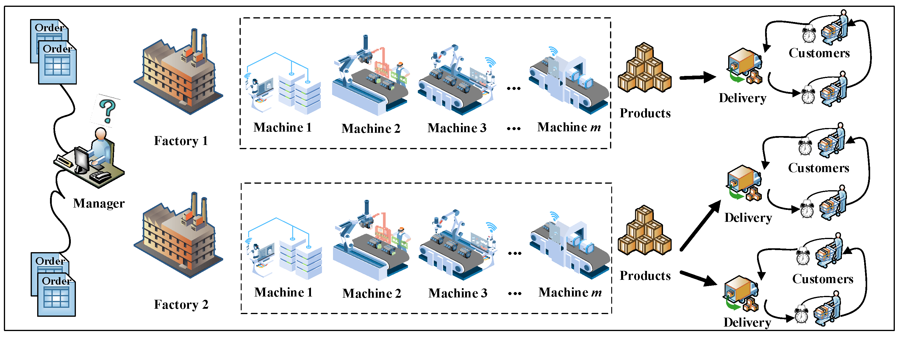
3.1. Problem Description

This work delves into a multi-objective IPDS with minimizing makespan and total weighted earliness and tardiness, consisting of two stages, namely the production stage and the distribution stage. The former comprises multiple identical factories, and each one is a flow shop. A specific set of jobs must be allocated across the flow shops, and each job must follow a fixed route on the machines at their respective flow shop. After processing, the jobs need to be shipped to customers located in different geographical areas via vehicles within time windows during the distribution stage. Consequently, to handle this problem, four decisions are made simultaneously, i.e., factory assignment of jobs, job processing sequence, vehicle allocation of jobs, and the job delivery sequence.

Note that a job is an order from a unique customer. Thus, the terms “job”, “order”, and “customer” are interchangeable as they are directly related to each other on a one-to-one basis. To clarify the problem being investigated, a visual example is shown in Figure 1 along with a mathematical model. A comprehensive listing of the related parameters and variables involved in constructing this model is provided in

Table 1. The parameters and variables.

Symbol	Description
$F$	Set of $f$ factories, $F=\left\{1,2,\dots ,f\right\}$.
$M$	Set of $m$ machines, $M=\left\{1,2,\dots ,m\right\}$.
$N$	Set of $n$ jobs, $N=\left\{0,1,2,\dots ,n\right\}$, where 0 means a virtual job.
$V$	Set of $v$ vehicles at a factory, $V=\left\{1,2,\dots ,v\right\}$.
$g$	The factory index, $g\in F$.
$i$	The machine index, $i\in M$.
$k,j,l$	The job index, $k,j,l\in N$.
$h$	The vehicle index, $h\in V$.
${\alpha }_{ij}$	The production time of job $j$ on machine $i$.
${\beta }_{kj}$	The drive time between customers $k$ and $j$.
${\gamma }_{gj}$	The drive time between factory $g$ and customer $j$.
${\psi }_j$	The load of job $j$.
${\phi }_j$	The service time at customer $j$.
$\left[d_j^{\prime },d_j^{″}\right]$	The delivery time window of customer $j$.
$E_j$	The unit earliness weight of customer $j$.
$T_j$	The unit tardiness weight of customer $j$.
$\varphi$	The maximum load capacity of the vehicle.
$G$	An extremely positive integer.
$X_{kjg}$	$=$1, if job $j$ is directly processed after job $k$ at factory $g$, 0, otherwise.
$Y_{jg}$	$=$1, if job $j$ is assigned to factory $g$, 0, otherwise.
$Z_{kjh}$	$=$1, if customer $j$ is directly delivered after customer $k$ by vehicle $h$, 0, otherwise.
$C_{ij}$	The completion time of job $j$ on machine $i$.
$S_h$	The delivery start time of vehicle $h$.
$A_j$	The arrival time at customer $j$.
$L_j$	The departure time from customer $j$.
$C_{max}$	The makespan criterion.
$TWET$	The total weighted earliness and tardiness criterion.

.

3.2. Mathematical Model

For a solution to be considered viable, it must adhere to the following restrictions:

• At time zero, all machines must be available for use;
• Once a machine processes a job, it cannot process another one;
• At no time can a single job be worked on by multiple machines;
• Interrupting a job that has already started on a machine is not allowed;
• Each customer is visited only once;
• Vehicles must obey capacity limits.

Using the definitions provided above, we constructed the mathematical model below.

$$\mathrm{Minimize} C_{max}$$

(1)

$$\mathrm{Minimize} TWET$$

(2)

s.t.

$${\displaystyle \sum }_{g\in F}{\displaystyle \sum }_{k\in N}{X}_{kjg}=1,\forall j\in N,j\ne 0,k\ne j$$

(3)

$${\displaystyle \sum }_{g\in F}{\displaystyle \sum }_{j\in N}{X}_{kjg}=1,\forall k\in N,k\ne j$$

(4)

$${\displaystyle \sum }_{g\in F}{Y}_{jg}=1,\forall j\in N,j\ne 0$$

(5)

$${\displaystyle \sum }_{k\in N}{X}_{kjg}+{\displaystyle \sum }_{l\in N}{X}_{jlg}\le 2·Y_{jg},\forall j\in N,j\ne 0,k\ne j\ne l,\forall g\in F$$

(6)

$${\displaystyle \sum }_{g\in F}\left(X_{kjg}+X_{jkg}\right)\le 1,\forall k,j\in N,k\ne j\ne 0$$

(7)

$$C_{ij}\ge C_{\left(i-1\right)j}+{\alpha }_{ij},\forall j\in N,j\ne 0,\forall i\in M$$

(8)

$$C_{ij}\ge C_{ik}+{\alpha }_{ij}+G·({\displaystyle \sum }_{g\in F}{X}_{kjg}-1),\forall k,j\in N,j\ne 0,k\ne j,\forall i\in M$$

(9)

$${\displaystyle \sum }_{h\in V}{\displaystyle \sum }_{j\in N}{Z}_{kjh}·Y_{kg}\le \left|V\right|,\forall g\in F,j\ne 0$$

(10)

$${\displaystyle \sum }_{h\in V}{\displaystyle \sum }_{k\in N}{Z}_{kjh}=1,\forall j\in N,j\ne 0$$

(11)

$${\displaystyle \sum }_{h\in V}{\displaystyle \sum }_{j\in N}{Z}_{kjh}=1,\forall k\in N,k\ne 0$$

(12)

$${\displaystyle \sum }_{k\in N}{Z}_{kjh}-{\displaystyle \sum }_{l\in N}{Z}_{jlh}=0,\forall j\in N,\forall h\in V$$

(13)

$${\displaystyle \sum }_{k\in N}{\displaystyle \sum }_{j\in N}{Z}_{kjh}·{\psi }_j\le \varphi ,\forall h\in V,k\ne j,j\ne 0$$

(14)

$${\displaystyle \sum }_{j\in N}{Z}_{0jh}·Y_{jg}\le 1,\forall h\in V,\forall g\in F, j\ne 0$$

(15)

$$S_h\ge C_{mj}+G·\left(Z_{kjh}-1\right),\forall k,j\in N,k\ne j,\forall h\in V$$

(16)

$$A_j\ge S_h+{\gamma }_{gj}+G·\left(Z_{0jh}+Y_{jg}-2\right),\forall j\in N,j\ne 0,\forall h\in V,\forall g\in F$$

(17)

$$A_j\ge L_k+{\beta }_{kj}+G·\left(Z_{kjh}-1\right),\forall k,j\in N,k\ne j\ne 0,\forall h\in V,\forall g\in F$$

(18)

$$L_j=A_j+{\phi }_j,\forall j\in N,j\ne 0$$

(19)

$$C_{max}\ge C_{mj},\forall j\in N,j\ne 0$$

(20)

$$TWET={{\displaystyle \sum }}_{j=1}^n\left(E_j\times max\left(d_j^{\prime }-A_j,0\right)+T_j\times max\left(L_j-d_j^{″},0\right)\right)$$

(21)

$$C_{ij}\ge 0,\forall i\in M,\forall j\in N,j\ne 0$$

(22)

$$X_{kjg}\in \left\{0,1\right\},\forall k,j\in N,k\ne j,\forall g\in F$$

(23)

$$Y_{jg}\in \left\{0,1\right\},\forall j\in N,j\ne 0,\forall g\in F$$

(24)

$$Z_{kjh}\in \left\{0,1\right\},\forall k,j\in N,k\ne j,\forall h\in V$$

(25)

$$A_j,L_j\ge 0,\forall j\in N,j\ne 0$$

(26)

The objective functions represented by Equations (1) and (2) are to minimize makespan and total weighted earliness and tardiness, respectively. The constraints laid out in Equations (3) and (4) dictate that there is precisely one preceding job and one succeeding job for each job on the machine. The constraint outlined in Equation (5) states that each job cannot be allocated to multiple factories simultaneously. Equation (6) signifies that each job owns at most one predecessor and one successor on a machine concurrently. Equation (7) mandates that there exists a strict ordering between two consecutive jobs. Equation (8) denotes that each job is worked on by only one machine at any given time. According to Equation (9), each machine must be dedicated to processing a single job at any given time. Equation (10) limits the number of vehicles. Equations (11) and (12) guarantee that no customer is visited multiple times. Equation (13) shows the constraint of maintaining continuity in vehicle routes. Equation (14) ensures that a vehicle’s maximum capacity limit is strictly observed. Equation (15) stipulates that no vehicle can be employed more than once. Equation (16) demonstrates the start time for vehicle delivery. Equations (17) and (18) provide information regarding when the vehicles arrive at customers, whereas Equation (19) determines when the vehicles depart from customers. Equations (20) and (21) define the makespan and total weighted earliness and tardiness, respectively. Equations (22)–(26) show the variable’s domain.

4. BSO and Q-Learning

4.1. BSO

Vitalized by the human inventive idea creation process, i.e., brainstorming process, Shi initially proposed a promising swarm-based metaheuristic: BSO [20]. The original BSO is straightforward in its design and can be easily implemented. Over the past years, BSO and its derivatives have achieved impressive results in tackling a range of complex problems, including real-parameter numerical optimization, distributed flow shops, and knowledge spillover problems [35,36,37,38,39,40]. Comprehensive experiments have verified that BSO possesses powerful performance to provide an outstanding compromise between exploration and exploitation abilities.

BSO begins with a population composed of multiple candidate individuals and each one means a solution to the optimization problem. Then, it performs three phases called the clustering phase, generating phase, and selecting phase to search solutions. The clustering phase involves using a clustering method to partition the population into several distinct clusters. For each cluster, the best individual in it is denoted as the center individual and the remaining are regarded as the normal ones. In the generating phase, new individuals are produced by employing one or two individuals from clusters. Each newly created individual is paired with an individual from the existing population. In the selecting phase, a selection method is adopted to store the better one from the paired individuals and save it for the next population. Finally, the three phases are iterated until a termination criterion is reached and the optimal solution is returned.

4.2. Q-Learning

Q-learning, as a typical model-free algorithm in RL, was originally introduced by Watkins and Dayan in 1992 [41]. Through a trial-and-error process, the method guides agents towards selecting the most beneficial behavior, and it comprises an environment, an agent, an action set, a state set, and a reward function. The main procedure of Q-learning is shown below. An agent selects an action $a_t$ in terms of its state $s_t$ at time $t$ in the environment. Then, it will obtain an immediate reward $r_{t+1}$ and its state will be transferred to a new state $s_{t+1}$. Meanwhile, the Q-table is updated according to Equation (27), where $Q\left(s_t,a_t\right)$ stands for the Q-value of conducting an action $a_t$ at state $s_t$, $\theta$ represents the learning rate, $\vartheta$ refers to the discount rate, and $\underset{a}{\max }Q\left(s_{t+1},a\right)$ means the biggest Q-value in the Q-table at state $s_{t+1}$.

$$Q\left(s_t,a_t\right)\leftarrow Q\left(s_t,a_t\right)+\theta ·\left[r_{t+1}+\vartheta ·\underset{a}{\max }Q\left(s_{t+1},a\right)-Q\left(s_t,a_t\right)\right]$$

(27)

The action selection is carried out in line with the Q-table. The values in an initial Q-table are equal to 0, in which the quantity of rows and columns matches the quantity of states and actions, respectively. The $ϵ$-greedy approach is commonly applied, and its details are described below. If a random value $r_v\in \left(0,1\right)$ is less than $ϵ$, then choose an action $a$ randomly. Otherwise, the action $a$ with a maximum Q-value is selected.

5. Presented MQBSO Algorithm

This section introduces the framework of MQBSO as follows: Step 1, initialize the population and parameters; Step 2, implement a dynamic clustering method to construct multiple clusters; Step 3, employ a Q-learning process to determine a search strategy for generating new individuals; Step 4, apply a selection approach to create the next population; and Step 5, update the population state and Q-table.

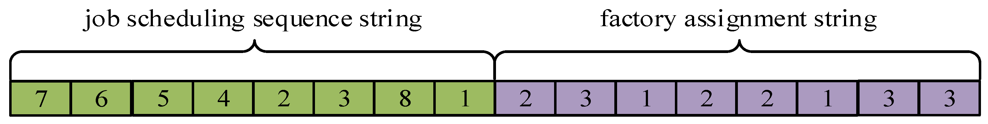
5.1. Solution Representation and Initial Population

A double-string representation method is employed to represent solutions, that is, individuals. The solution is denoted as a job scheduling sequence string $\left[{\pi }_1,{\pi }_2,\dots ,{\pi }_n\right]$ and a factory assignment string $\left[{\omega }_1,{\omega }_2,\dots ,{\omega }_n\right]$, where ${\pi }_j$ indicates a job index, $j\in \left\{1,2,\dots ,n\right\}$, ${\pi }_j\in \left\{1,2,\dots ,n\right\}$, ${\omega }_j$ means a factory index assigned to the job located at the $j$-th position in the job scheduling sequence string, ${\omega }_j\in \left\{1,2,\dots ,f\right\}$. To better clarify this method, Figure 2 provides a visual example using a scenario where eight jobs are assigned to three factories. In it, jobs 5 and 3 are handled in factory 1, jobs 7, 4, and 2 are assigned to factory 2, and the rest belong to factory 3.

Note that the aforementioned approach only focuses on assigning jobs to factories without obtaining other decisions, namely, the sequence in which jobs are processed on machines, allocation of vehicles for jobs, and delivery sequence of jobs. To convert the solution into an actionable plan, we present the following rules:

• Jobs that have been allocated to a factory are processed in a sequence that matches their assigned order on the machines;
• After the production of jobs, they are assigned in a sequential manner to a vehicle. The earlier the processing is completed, the sooner the vehicle is assigned. Meanwhile, vehicles are required not to exceed their maximum load capacity.
• Jobs are transported in the exact sequence in which they are loaded into the vehicle.

According to the above method and rules, we can successfully transform a solution into practicable decisions.

Ensuring both the stability and diversity of MQBSO, this work adopts a random method to initialize $p_s$ feasible solutions for constructing the initial population.

5.2. Clustering

Along with the evolution of BSO, the population should be gathered into various numbers of clusters during the iteration. Thus, this work develops a dynamic clustering approach driven by a nondominated sorting method [42]. This work sorts all individuals in the population and assigns them sorted values based on their dominated relationships. The smaller the sorted value, the better the individual. Hence, this work sets the best individuals with the smallest sorted value of 1 as the center individuals, while the rest as normal individuals. For each center individual, this work constructs a cluster. To conduct such work, the normal ones are randomly assigned to these clusters. Notice that when only one individual has the sorted value of 1, this work selects the individuals with the sorted value of 2 as center individuals.

5.3. Generating

Generating is the core process of BSO, which controls the global search and local search abilities of an algorithm through applying one individual or two individuals in clusters. In this process, three vital parameters are used, i.e., $r_g$, $r_o$, $r_t$. Let $r_g$ decide whether a new individual is constructed by one individual or two individuals. $r_o$ determines whether a new individual is created by utilizing one center individual or one normal individual. $r_t$ decides whether a new individual is produced via employing two center individuals or two normal ones. Based on them, this work introduces a global search strategy and a local search strategy. The details about them are provided as follows:

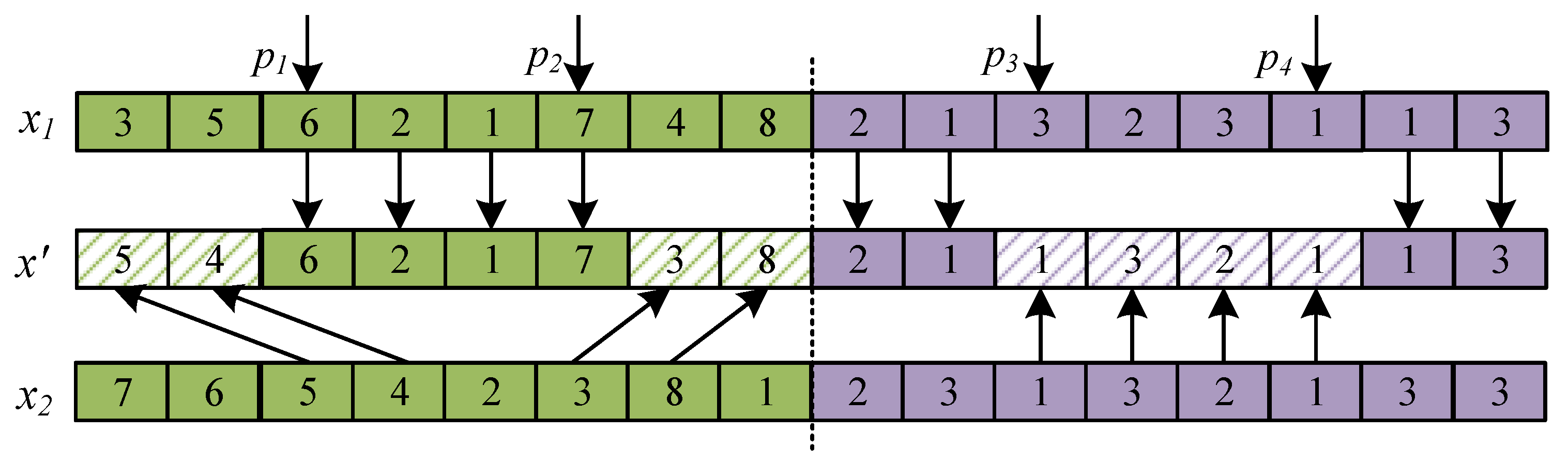
• A global search strategy is designed when utilizing two randomly chosen center or normal individuals to construct new individuals, where the sequence-based [43] and the two-point crossover [44] methods are adopted. The former is applied to update the job scheduling sequence string and the latter is utilized to update the factory assignment string. The main contents of these two methods are described below.
• Sequence-based crossover method: First, randomly have two job position indexes $p_1$, $p_2$. Then, jobs between them in the individual $x_1$ are copied to the same positions of a new individual $x^{\prime }$. Finally, the missing jobs in $x^{\prime }$ are added as their appearance in the individual $x_2$. Hence, the job scheduling sequence string of $x^{\prime }$ is obtained. Two-point crossover method: First, two factory position indexes $p_3$, $p_4$ are generated at random. Then, extract factory assignments beyond $p_3$ and $p_4$ in $x_1$ and place them into the same positions of $x^{\prime }$. Finally, the rest factory assignments in $x^{\prime }$ are filled with the elements at the same positions of $x_2$. Thus, the factory assignment string of $x^{\prime }$ is acquired. By employing these two methods, a new individual is successfully produced. To clearly exhibit the generation process, Figure 3 depicts an illustrative example.
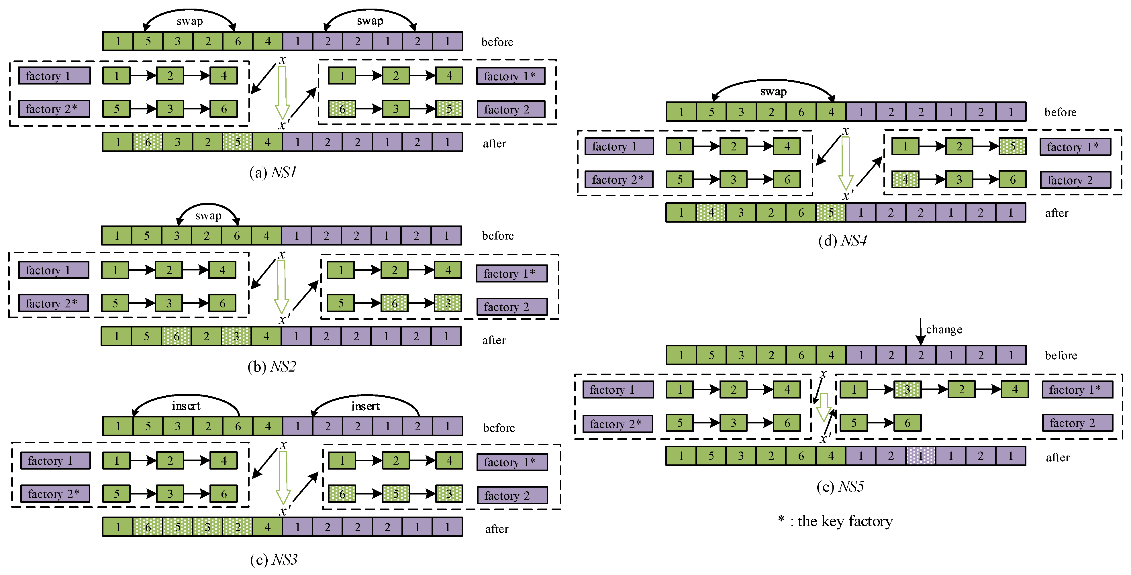
• A local search strategy is developed when using one randomly selected center or normal individual to construct new individuals, where five kinds of neighborhood structures, named NS1, NS2, NS3, NS4, and NS5 are introduced. The main idea of NS1 is as follows: randomly produce two job positions for a chosen individual, then swap these two jobs and exchange their respective factory assignments.

Different from NS1, the problem-dependent information is considered for the final four neighborhood structures. Given that one of the primary objectives of the problem investigated is to optimize the makespan criterion, it is essential to focus on improving the performance of the key factory that has a maximum completion time. To reach this, it is vital to adjust both the factory assignment and job processing sequence associated with this factory. According to the key factory theory [45] and the characteristics of the presented problem, this work designs four problem-dependent neighborhood structures. The details about them are given as follows: NS2 randomly swaps two jobs in the key factory; NS3 employs an insert operator, where two jobs in the key factory are randomly chosen, and one of which is inserted into the front of the other, along with corresponding changes are made to their factory assignments; NS4 is similar to NS2 except that the factory assignment of the two jobs is different, and one must be the key factory; and NS5 changes the factory assignment of a job in the key factory.

It is worth mentioning that for each chosen center or normal individual, only one of five neighborhood structures is selected at random to produce a new individual. This work stores the better one between the chosen and new individuals in accordance with their dominated relationship. To intuitively understand the five neighborhood structures, Figure 4 shows five examples of these structures, and the key factory is denoted as “*”.

Furthermore, to avoid premature convergence and enhance the local search ability, we adopt a simulated annealing strategy [46]. The steps of this strategy are outlined below.

Step 1: Set an initial temperature $T_0=0.5·\left({\sum }_{i=1}^m{\sum }_{j=1}^n{\alpha }_{ij}/\left(10·n·m\right)\right)$, a final temperature $T_{min}=0.5·T_0$, and update the current temperature $T:=T_0$.

Step 2: Select a center or normal individual $x$ at random and set an intermediary individual $x_3:=x$.

Step 3: Randomly perform one of the five neighborhood structures on $x_3$ to generate a new individual $x^{\prime }$.

Step 4: If $x^{\prime }$ dominates $x_3$, $x_3:=x^{\prime }$; otherwise, $x_3:=x_3$.

Step 5: Adjust the temperature according to the formula: $T:=T-\left(T·0.1\right)$, and repeat Steps 3–5 until $T\le T_{min}$.

Step 6: Generate the new individual $x^{\prime }:=x_3$ and save it.

In the generating phase, Q-learning is implemented to assist MQBSO in choosing a generation strategy, the introduction of this process is described in Section 5.5.

5.4. Selecting

In the original BSO, the selecting phase is performed to store better individuals to enter the next population. It usually saves the better ones between new individuals and their connected individuals in the population. This method may discard some better individuals. In order to strengthen MQBSO’s capability to explore promising directions, this work employs an effective selection method [44] by utilizing the nondominated sorting and crowding distance approaches. The basic idea of this method is shown as follows: First, merge the existing population with new individuals; second, sort all individuals and calculate their crowding distance values; and finally, extract the best $p_s$ individuals as the next population based on their sorted and crowding distance values.

5.5. Q-Learning Process

In this work, Q-learning is composed of four actions, four states, a reward function, and an action selection method. Four actions are defined as the combinations of a global search strategy, a local search strategy, and a simulated annealing strategy. Four states are described by the convergence and uniformity metrics. A reward function is designed based on the states and an improved $\epsilon$-greedy method is newly developed.

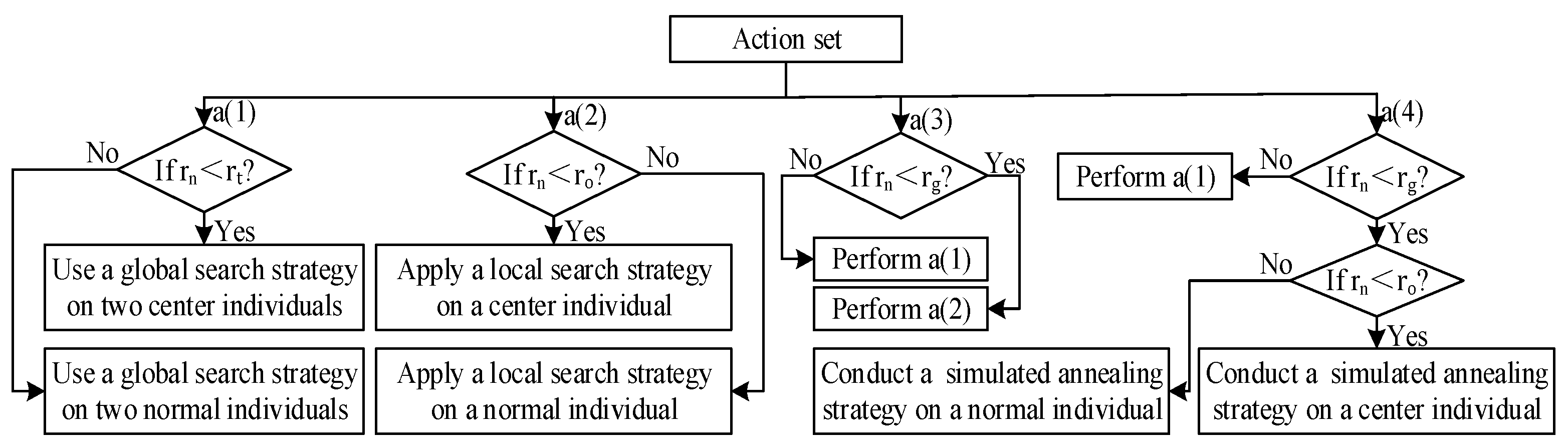
5.5.1. Action Set

The action set consists of four actions, and each one is a combination of a global search strategy, a local search strategy, and a simulated annealing strategy. Action $a\left(1\right)$ contains a global search strategy. Action $a\left(2\right)$ includes a local search strategy. Action $a\left(3\right)$ is composed of a global search strategy and a local search strategy. Action $a\left(4\right)$ is made up of a global search strategy and a simulated annealing strategy. According to the above designs, Figure 5 gives the framework of an action set in MQBSO, where $r_n$ denotes a random number between $\left(0,1\right)$.

This work uses an improved $\epsilon$-greedy method [32] to conduct the selection of an action, where $\epsilon$ is calculated by Equation (28). In Equation (28), ${\rho }_c$ denotes the current number of fitness function evaluations, and ${\rho }_{max}$ represents a stopping condition equaling to $150·n·m$ fitness function evaluations. Randomly generate a float number $\lambda \in \left(0,1\right)$, if $\lambda$ is bigger than $1-\epsilon$, one of four actions is chosen at random; otherwise, the agent selects the action with the highest Q-value as its preferred option. This method ensures that the selection probability of the two cases is about half in the beginning, along with the agent maintaining a certain ability to explore during the early stage. As the algorithm evolves, the action with the highest Q-value is favored. Thus, MQBSO can effectively intensify the exploration ability and reduce the possibility of dropping into local optima.

$$\epsilon =0.5/\left(1+e^{\left(10·\left({\rho }_c-0.6·{\rho }_{max}\right)\right)/{\rho }_{max}}\right),$$

(28)

5.5.2. State Set

To clearly depict the state, a convergence index (C-metric) [47] and a uniformity index (D-metric) [33] are used, which are computed based on the formulas defined below.

$$C\left(U,W\right)=\left|\left\{w\in W|\exists u\in U:u\prec w\right\}\right|/\left|W\right|$$

(29)

As per Equation (29), $U$ and $W$ refer to the sets of non-dominated solutions acquired in the $\mu$-th and $\left(\mu -1\right)$-th iterations. $C(U,W)$ quantifies the percentage of solutions in set $W$ which are dominated by solutions within set $U$, and $\left|W\right|$ stands for the size of $W$. Generally, a bigger $C\left(U,W\right)$ suggests that the performance of set $U$ is better.

$$D={\displaystyle \left|{\sum }_{e=1}^{\left|E\right|}{z}_e-\overline{z}\right|}/\left|\left|E\right|·\overline{z}\right|,$$

(30)

$$\overline{z}={\sum }_{e=1}^{\left|E\right|}{z}_e/\left|E\right|,$$

(31)

As per Equation (30), $E$ is a non-dominated solution set and $\left|E\right|$ indicates its size. $z_e$ refers to the shortest Euclidean distance from the $e$-th solution and any other solution in $E$, and $\overline{z}$ means the average distance as measured using the formula presented in Equation (31). Usually, a higher D-metric value implies a better performance of uniformity.

$$∆D(U,W)=D\left(U\right)-D\left(W\right)$$

(32)

The occurrence percentage of $C(U,W)>0$, $C(U,W)\le 0$, $∆D(U,W)>0$, and $∆D(U,W)\le 0$ in the entire search process of MQBSO on four instances are displayed in Figure 6. We see that each of the four cases appear. As a result, it is rational to consider four combinations of $C(U,W)$ and $∆D(U,W)$ as four states, i.e., $s\left(1\right)$: $C(U,W)>0$ and $∆D(U,W)>0$, $s\left(2\right)$:$C(U,W)>0$ and $∆D(U,W)\le 0$, $s\left(3\right)$: $C(U,W)\le 0$ and $∆D(U,W)>0$, and $s\left(4\right)$: $C(U,W)\le 0$ and $∆D(U,W)\le 0$.

5.5.3. Reward

In this work, four states are labeled as $s\left(1\right)$, $s\left(2\right)$, $s\left(3\right)$, and $s\left(4\right)$. The bigger the label value of the state, the worse the state. $s\left(1\right)$ means the best state while $s\left(4\right)$ is the worst one. Thus, rewards are set based on the label value of states. Four reward values $r_v$ are 5, 3, 3, and 1 for these four states, respectively.

After a detailed discussion, Algorithm 1 provides the main procedure of MQBSO.

Algorithm 1: MQBSO

Input: Population size $p_s$, three generation parameters $r_g$, $r_o$, $r_t$, learning rate $\theta$, discount rate $\vartheta$, and a stopping condition ${\rho }_{max}$.

Output: A non-dominated solution set.

Initialize the population and parameters (c.f. Section 5.1)

While the stopping condition is not reached do

Implement a dynamic clustering method in the clustering phase (c.f. Section 5.2).

Employ a Q-learning process in the generating phase (c.f. Section 5.3 and Section 5.5).

Apply a selection method in the selecting phase (c.f. Section 5.4).

Update the population state and Q-table.

End while

6. Experimental Evaluations

In this section, comparison experiments and statistical tests are conducted to study MQBSO’s performance. MQBSO and comparison algorithms are programmed in C++ and performed on a personal computer equipped with HUAWEI Core i5-8265U CPU and 8 GB RAM in Qingdao, China. Four comparison methods are well-known metaheuristics: multi-objective whale swarm algorithm (MOWSA) [43], multi-objective brain storm optimization (MOBSO) [44], nondominated sorting genetic algorithm II (NSGA-II) [42], and multi-objective evolutionary algorithm based on decomposition (MOEA/D) [48]. In fairness, this work sets $150·n·m$ fitness function evaluations as a termination criterion, and all methods independently solve each instance 20 times.

6.1. Test Instances

Since the previous work does not address the presented problem, we cannot find available benchmarks. Therefore, we produce a set of instances based on the problems’ features. The benchmarks regarding flow shop scheduling and vehicle routing problems are employed to construct instances, i.e., the VFR benchmark [49] for the former, and the Gehring & Homberger benchmark [50] for the latter.

In the VFR benchmark, “VFRa_b_c” means the $c$-th instance of a test problem having $a$ jobs and $b$ machines. Four instances are adopted, including VFR30_5_1, VFR30_10_1, VFR60_5_1, and VFR60_10_1, respectively. The instances VFR90_5_1, VFR90_10_1, VFR120_5_1, and VFR120_10_1 do not exist in the VFR benchmark. Thus, this work creates them by applying the information of the first 90, 120 jobs and the first 5, 10 machines regarding the VFR100_20_1 and VFR200_20_1.

In the Gehring & Homberger benchmark, an instance named C1_2_1 is applied, where coordinates, time windows, and service times are provided. Through choosing the first 30, 60, 90, and 120 customers from it, four instances, namely, C1_2_1, C1_2_1, C1_2_1, and C1_2_1 are obtained. The chosen instances contain eight combinations of $n\times m$: $\left(\mathrm{30,60,90,120}\right)\times \left(\mathrm{5,10}\right)$, where $n$ and $m$ indicate the number of jobs and machines, respectively. This work sets the number of factories $f\in \left\{\mathrm{2,3},4\right\}$. Hence, a total of 24 test instances are successfully generated.

For convenience,

Table 2. Abbreviation information of 24 test instances.

Instance	$\mathit{f}$	Production	Distribution	Instance	$\mathit{f}$	Production	Distribution
2-5-30	2	VFR30_5_1	C1_2_1	2-10-30	2	VFR30_10_1	C1_2_1
2-5-60	2	VFR60_5_1	C1_2_1	2-10-60	2	VFR60_10_1	C1_2_1
2-5-90	2	VFR90_5_1	C1_2_1	2-10-90	2	VFR90_10_1	C1_2_1
2-5-120	2	VFR120_5_1	C1_2_1	2-10-120	2	VFR120_10_1	C1_2_1
3-5-30	3	VFR30_5_1	C1_2_1	3-10-30	3	VFR30_10_1	C1_2_1
3-5-60	3	VFR60_5_1	C1_2_1	3-10-60	3	VFR60_10_1	C1_2_1
3-5-90	3	VFR90_5_1	C1_2_1	3-10-90	3	VFR90_10_1	C1_2_1
3-5-120	3	VFR120_5_1	C1_2_1	3-10-120	3	VFR120_10_1	C1_2_1
4-5-30	4	VFR30_5_1	C1_2_1	4-10-30	4	VFR30_10_1	C1_2_1
4-5-60	4	VFR60_5_1	C1_2_1	4-10-60	4	VFR60_10_1	C1_2_1
4-5-90	4	VFR90_5_1	C1_2_1	4-10-90	4	VFR90_10_1	C1_2_1
4-5-120	4	VFR120_5_1	C1_2_1	4-10-120	4	VFR120_20_1	C1_2_1

provides abbreviations for the 24 test instances. In it, the first instance called “2-5-30” consists of 2 factories, 5 machines, and 30 jobs, in which the production and distribution data are from VFR30_5_1 and C1_2_1, respectively. The remaining can be deduced by analogy. Furthermore, this work sets the load of jobs from an interval [10,40], the maximum load capacity of vehicles is 100, 125, 150, and 200 when the quantity of jobs is 30, 60, 90, and 120, respectively, and the unit earliness and tardiness weights of jobs are generated at random from $\left\{\mathrm{0.1,0.2,0.3,0.4,0.5}\right\}$.

6.2. Parameters Setting

An orthogonal experiment method [51] is employed in this research to implement the parameter experiment on a moderate-size instance named “3-5-60” with 3 factories, 5 machines and 60 jobs. This method is viewed as a modern technique for analyzing and optimizing parameters across various research fields. Generally, practical engineering design and optimization tasks require the consideration of three or more influential factors, leading to the application of full factorial design analysis. MQBSO considers four parameters, i.e., $p_s$, $r_g$, $r_o$, and $r_t$. Each parameter has four levels: $p_s\in \left\{\mathrm{20,40,60,80}\right\}$, $r_g\in \left\{\mathrm{0.20,0.40,0.60,0.80}\right\}$, $r_o\in \left\{\mathrm{0.20,0.40,0.60,0.80}\right\}$, $r_t\in \left\{\mathrm{0.20,0.40,0.60,0.80}\right\}$, and an array ${L_{16}}_4^4$ containing 16 combinations is created. To promote fairness in the comparison of different algorithms, this work sets the same number of fitness function evaluations as a stopping condition, i.e., $150·n·m$, where $n$ and $m$ are the quantity of jobs and machines, respectively. Each combination is executed 20 times individually and the results are analyzed by applying the IGD-metric. The average IGD (AIGD) results are calculated and provided in

Table 3. Orthogonal array and AIGD results of MQBSO.

No.	${\mathit{p}}_{\mathit{s}}$	${\mathit{r}}_{\mathit{g}}$	${\mathit{r}}_{\mathit{o}}$	${\mathit{r}}_{\mathit{t}}$	AIGD
1	20	0.20	0.20	0.20	0.1016
2	20	0.40	0.40	0.40	0.0927
3	20	0.60	0.60	0.60	0.0904
4	20	0.80	0.80	0.80	0.0861
5	40	0.20	0.40	0.60	0.1056
6	40	0.40	0.20	0.80	0.0852
7	40	0.60	0.80	0.20	0.0909
8	40	0.80	0.60	0.40	0.1232
9	60	0.20	0.60	0.80	0.1005
10	60	0.40	0.80	0.60	0.0952
11	60	0.60	0.20	0.40	0.0939
12	60	0.80	0.40	0.20	0.0984
13	80	0.20	0.80	0.40	0.0931
14	80	0.40	0.60	0.20	0.0956
15	80	0.60	0.40	0.80	0.0868
16	80	0.80	0.20	0.60	0.0867

. Through analyzing the obtained results, a hopeful parameter combination is produced, i.e., $p_s=40$, $r_g=0.40$, $r_o=0.20$, $r_t=0.80$.

Similarly, the parameters of four peers are achieved via using the same method, and their parameters are displayed in

Table 4. Parameter settings of four compared algorithms.

Algorithm	Parameter	Levels	Value
MOWSA	population size	20, 40, 60, 80	20
	crossover probability	0.80, 0.85, 0.90, 0.95	0.85
	mutation probability	0.10, 0.15, 0.20, 0.25	0.15
MOBSO	$p_s$	20, 40, 60, 80	80
	$r_g$	0.20, 0.40, 0.60, 0.80	0.80
	$r_o$	0.20, 0.40, 0.60, 0.80	0.20
	$r_t$	0.20, 0.40, 0.60, 0.80	0.60
NSGA-II	population size	20, 40, 60, 80	80
	mutation probability	0.10, 0.15, 0.20, 0.25	0.15
MOEA/D	population size	20, 40, 60, 80	40
	neighborhood size	10, 15, 20, 25	25

. In addition, the learning rate $\theta$ and discount rate $\vartheta$ are set by drawing on existing research [32], which are 0.5 and 0.8, respectively.

6.3. Performance Metrics

Convergence and uniformity are two significant measures for examining the efficiency of multi-objective algorithms. Hence, this work utilizes three common performance metrics to carry out algorithmic measurements, i.e., C-metric [47], Inverted Generational Distance-metric (IGD-metric) [47], and Hypervolume-metric (HV-metric) [52]. The C-metric is defined in Equation (29), and the details of the IGD- and HV-metrics are offered below.

The IGD-metric is applied to reflect both convergence and uniformity of a method and its calculation formula is shown as:

$$IGD\left(P^{*},P\right)={\sum }_{p\in P^{*}}dist\left(p,P\right)/\left|P^{*}\right|$$

(33)

where $P$ and $P^{\mathrm{*}}$ mean an obtained solution set by an algorithm and the Pareto optimal front, respectively. In reality, the Pareto optimal front is difficult to achieve for the examined problem. Hence, this work generates $P^{\mathrm{*}}$ by merging the obtained solution sets of all employed algorithms and discarding the dominated solutions. $dist\left(p,P\right)$ represents the shortest Euclid distance from a solution $p$ in $P^{\mathrm{*}}$ and any other solution in $P$, and $\left|P^{\mathrm{*}}\right|$ is the quantity of solutions in $P^{\mathrm{*}}$. In this work, all objective values are normalized within $\left(\mathrm{0,1}\right)$, and an algorithm with lower IGD-metric values is ideal.

The HV-metric is also used to account for the convergence and uniformity of an algorithm. It estimates the volume of the area covered by the obtained nondominated solutions of an algorithm and a known reference point $H^{*}$. It is calculated as:

$$HV=\delta \left({\cup }_{o=1}^{\left|O\right|}{sv}_o\right)$$

(34)

where the Lebesgue measure $\delta$ is implemented to determine the volume of a set. $\left|O\right|$ denotes the quantity of solutions in the solution set $O$, and ${sv}_o$ is the super volume of the area coved by the $o$-th solution in $O$ and $P^{*}$. As in the IGD-metric, the obtained objective values of all algorithms are transformed into the range of $\left(\mathrm{0,1}\right)$, and $H^{*}$ is $\left(\mathrm{1,1}\right)$. Generally, a larger HV-metric value shows a better performance.

6.4. Experimental Results and Analysis

This section compares MQBSO with its four rivals on the C-metric, IGD-metric, and HV-metric. The four peers are, respectively, MOWSA, MOBSO, NSGA-II, and MOEA/D, and the results are presented in

Table 5. Results of MQBSO and its peers concerning C-metric.

Instance	C(QB,WS)	C(WS,QB)	C(QB,BS)	C(BS,QB)	C(QB,GA)	C(GA,QB)	C(QB,EA)	C(EA,QB)
2-5-30	0.7951	0.0161	0.9908	0.0000	0.9889	0.0000	0.9709	0.0031
2-5-60	0.9810	0.0000	0.9729	0.0000	1.0000	0.0000	1.0000	0.0000
2-5-90	0.9735	0.0000	1.0000	0.0000	1.0000	0.0000	1.0000	0.0000
2-5-120	0.9389	0.0000	0.9739	0.0018	0.9818	0.0000	1.0000	0.0000
2-10-30	0.0000	0.6810	0.0065	0.5785	0.0439	0.2361	0.0696	0.2504
2-10-60	0.9481	0.0000	1.0000	0.0000	1.0000	0.0000	1.0000	0.0000
2-10-90	0.9297	0.0000	1.0000	0.0000	1.0000	0.0000	1.0000	0.0000
2-10-120	0.9569	0.0000	1.0000	0.0000	1.0000	0.0000	1.0000	0.0000
3-5-30	0.9782	0.0000	0.9519	0.0000	0.8082	0.1250	0.6868	0.2206
3-5-60	0.9306	0.0000	0.9731	0.0000	1.0000	0.0000	0.9750	0.0000
3-5-90	0.9816	0.0000	1.0000	0.0000	1.0000	0.0000	1.0000	0.0000
3-5-120	0.9687	0.0024	0.9964	0.0000	1.0000	0.0000	1.0000	0.0000
3-10-30	0.1077	0.5823	0.2163	0.5048	0.4705	0.2068	0.3565	0.2504
3-10-60	0.9921	0.0000	1.0000	0.0000	1.0000	0.0000	1.0000	0.0000
3-10-90	0.9658	0.0000	1.0000	0.0000	1.0000	0.0000	1.0000	0.0000
3-10-120	0.9764	0.0000	1.0000	0.0000	1.0000	0.0000	1.0000	0.0000
4-5-30	0.8991	0.0000	0.9064	0.0000	0.1531	0.7797	0.0640	0.8341
4-5-60	0.9820	0.0000	0.9753	0.0000	0.9952	0.0000	1.0000	0.0000
4-5-90	0.9792	0.0000	0.9957	0.0000	1.0000	0.0000	1.0000	0.0000
4-5-120	0.9464	0.0000	0.9918	0.0000	1.0000	0.0000	1.0000	0.0000
4-10-30	0.6849	0.0225	0.9400	0.0038	0.1859	0.4120	0.1172	0.4602
4-10-60	0.9605	0.0000	1.0000	0.0000	1.0000	0.0000	1.0000	0.0000
4-10-90	0.9796	0.0000	1.0000	0.0000	1.0000	0.0000	1.0000	0.0000
4-10-120	0.9796	0.0000	0.9981	0.0000	1.0000	0.0000	1.0000	0.0000
Average	0.8682	0.0543	0.9120	0.0454	0.8595	0.0733	0.8433	0.0841

,

Table 6. Results of MQBSO and its peers about IGD-metric.

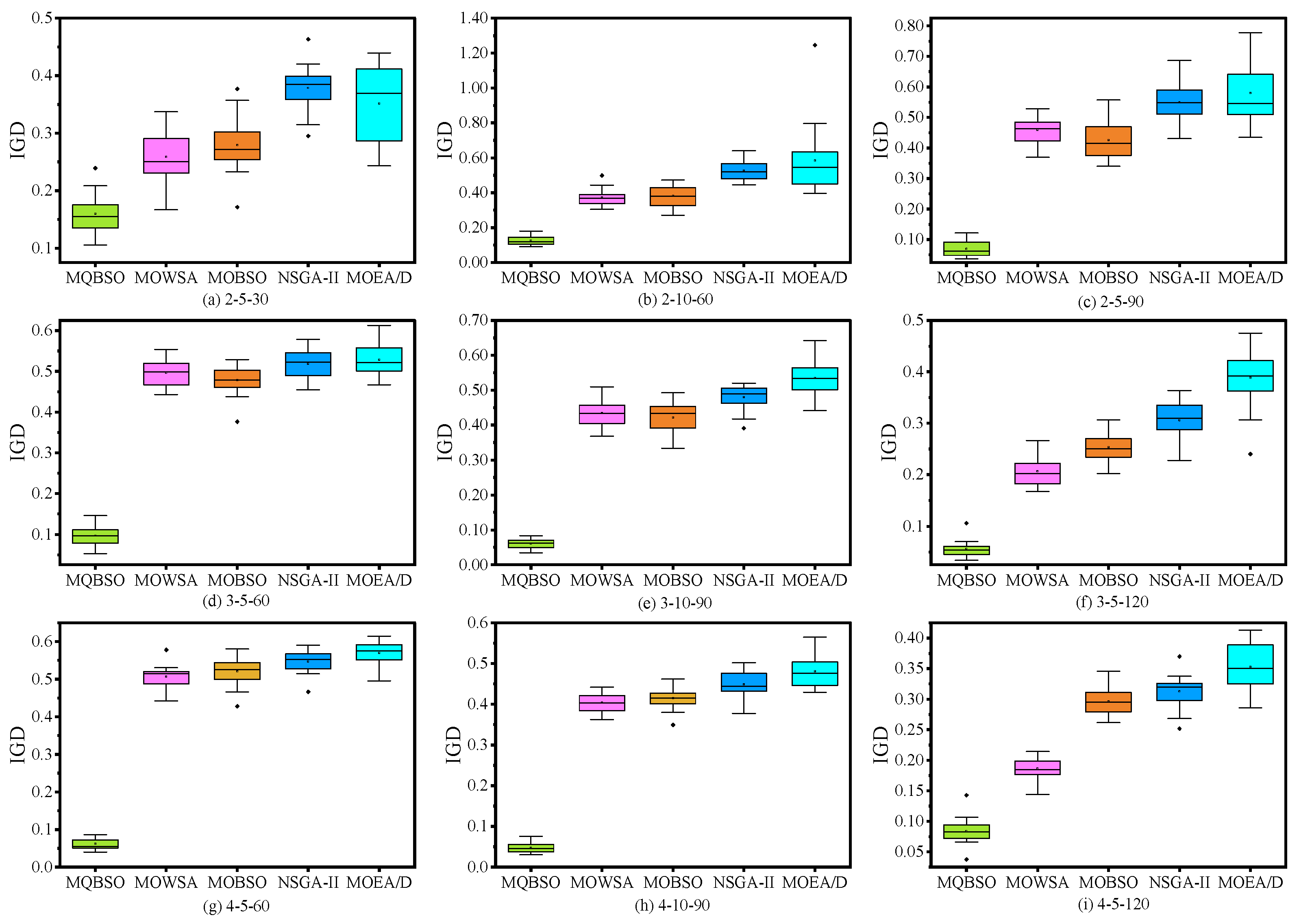
Instance	MQBSO	MOWSA	MOBSO	NSGA-II	MOEA/D
2-5-30	0.1595	0.2585	0.2788	0.3784	0.3512
2-5-60	0.0668	0.4456	0.4132	0.5073	0.4948
2-5-90	0.0695	0.4587	0.4252	0.5485	0.5790
2-5-120	0.0946	0.2911	0.2813	0.4224	0.4837
2-10-30	0.4201	0.1777	0.2311	0.3187	0.3576
2-10-60	0.1246	0.3708	0.3807	0.5254	0.5820
2-10-90	0.1147	0.3676	0.4778	0.6540	0.9409
2-10-120	0.1023	0.3686	0.4377	0.6161	0.7933
3-5-30	0.1038	0.3638	0.3531	0.2781	0.2269
3-5-60	0.0963	0.4956	0.4784	0.5185	0.5287
3-5-90	0.0466	0.4270	0.4263	0.4711	0.4883
3-5-120	0.0558	0.2064	0.2535	0.3055	0.3883
3-10-30	0.1799	0.1421	0.1626	0.2380	0.2398
3-10-60	0.0561	0.4702	0.4462	0.5000	0.5307
3-10-90	0.0603	0.4344	0.4224	0.4797	0.5345
3-10-120	0.0506	0.2067	0.2748	0.3302	0.4071
4-5-30	0.2378	0.4851	0.4845	0.1161	0.1381
4-5-60	0.0616	0.5063	0.5201	0.5465	0.5696
4-5-90	0.0646	0.4412	0.4888	0.5184	0.5581
4-5-120	0.0842	0.1863	0.2955	0.3124	0.3523
4-10-30	0.1882	0.2383	0.2371	0.2016	0.2659
4-10-60	0.0511	0.4222	0.4571	0.4807	0.5007
4-10-90	0.0471	0.4030	0.4150	0.4480	0.4806
4-10-120	0.0477	0.2245	0.2720	0.3113	0.3809
Average	0.1077	0.3497	0.3714	0.4178	0.4655

and

Table 7. Results of MQBSO and its peers regarding HV-metric.

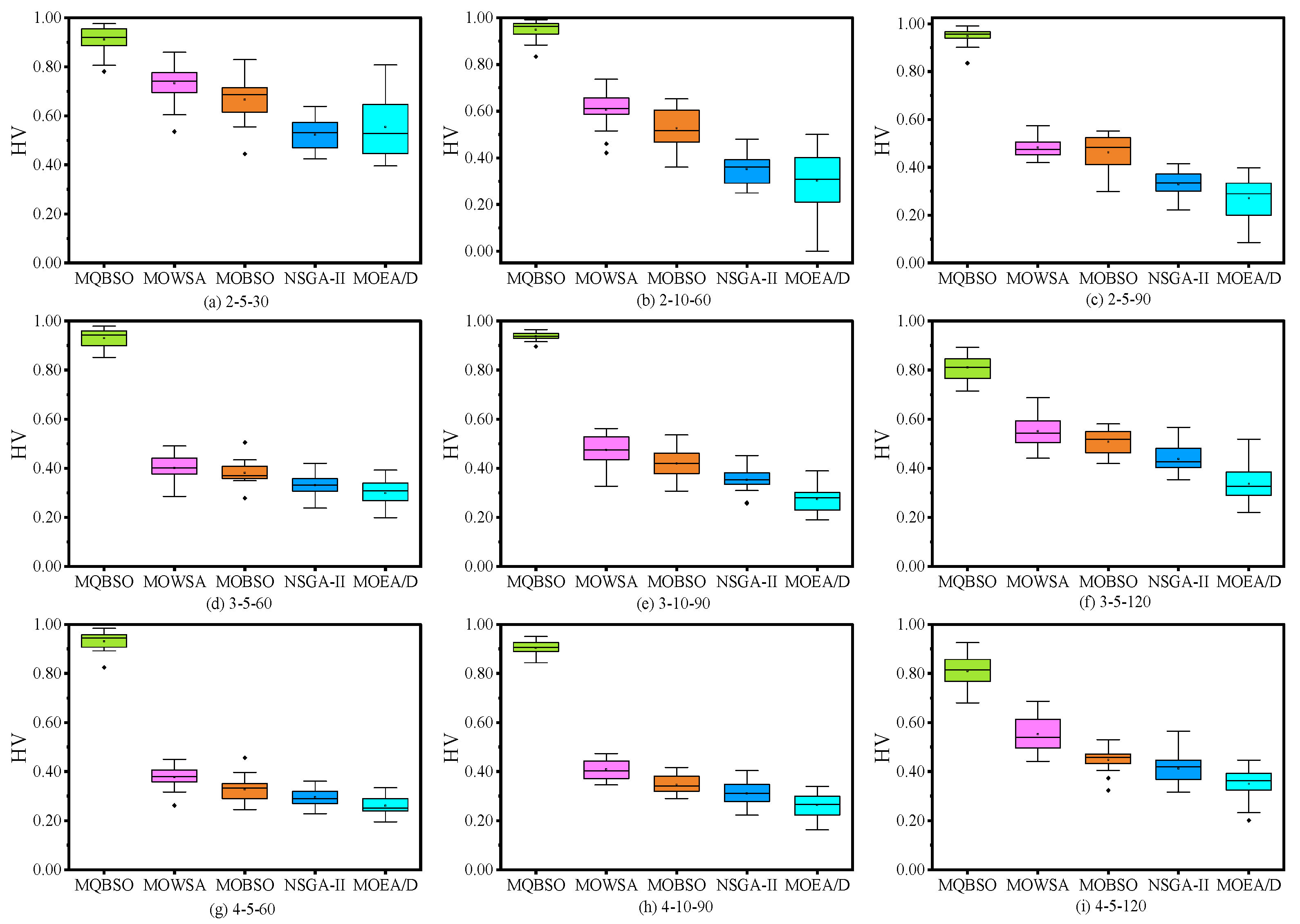
Instance	MQBSO	MOWSA	MOBSO	NSGA-II	MOEA/D
2-5-30	0.9106	0.7331	0.6655	0.5222	0.5543
2-5-60	0.9537	0.5126	0.4992	0.3914	0.3804
2-5-90	0.9474	0.4825	0.4625	0.3292	0.2711
2-5-120	0.8697	0.5955	0.5678	0.3848	0.3024
2-10-30	0.3208	0.8071	0.7052	0.5291	0.5064
2-10-60	0.9489	0.6054	0.5272	0.3515	0.3027
2-10-90	0.9615	0.6476	0.4196	0.2637	0.0894
2-10-120	0.9062	0.5797	0.4067	0.2397	0.1076
3-5-30	0.8422	0.5379	0.4982	0.6579	0.6860
3-5-60	0.9302	0.4018	0.3822	0.3312	0.2990
3-5-90	0.9177	0.4260	0.4011	0.3464	0.3141
3-5-120	0.8111	0.5519	0.5074	0.4383	0.3359
3-10-30	0.5548	0.7481	0.6640	0.5827	0.5695
3-10-60	0.9583	0.4643	0.4265	0.3714	0.3171
3-10-90	0.9385	0.4756	0.4193	0.3525	0.2742
3-10-120	0.7802	0.5197	0.4477	0.3680	0.2821
4-5-30	0.7839	0.4464	0.4105	0.8864	0.8946
4-5-60	0.9305	0.3777	0.3268	0.2951	0.2602
4-5-90	0.9097	0.3970	0.3596	0.3166	0.2671
4-5-120	0.8098	0.5521	0.4477	0.4121	0.3497
4-10-30	0.6532	0.5663	0.5291	0.8053	0.8131
4-10-60	0.9167	0.4544	0.3952	0.3578	0.3262
4-10-90	0.9036	0.4083	0.3459	0.3110	0.2636
4-10-120	0.7958	0.5252	0.4558	0.4019	0.3179
Average	0.8440	0.5340	0.4696	0.4269	0.3785

.

Table 5 exhibits the comparison results concerning C-metric, where the symbols “QB”, “WS”, “BS”, “GA”, and “EA” indicate the nondominated solution sets obtained by MQBSO, MOWSA, MOBSO, NSGA-II, and MOEA/D, respectively. A higher value of $\mathrm{C}\left(\mathrm{Q}\mathrm{B},\mathrm{R}\right)$ suggests a superior performance of MQBSO, $\mathrm{R}\in \left\{\mathrm{W}\mathrm{S},\mathrm{B}\mathrm{S},\mathrm{G}\mathrm{A},\mathrm{E}\mathrm{A}\right\}$. As shown in Table 5, the values of $\mathrm{C}\left(\mathrm{Q}\mathrm{B},\mathrm{W}\mathrm{S}\right)$ and $\mathrm{C}\left(\mathrm{Q}\mathrm{B},\mathrm{B}\mathrm{S}\right)$ are bigger than those of $\mathrm{C}\left(\mathrm{W}\mathrm{S},\mathrm{Q}\mathrm{B}\right)$ and $\mathrm{C}\left(\mathrm{B}\mathrm{S},\mathrm{Q}\mathrm{B}\right)$ in 22 instances, along with the values of $\mathrm{C}\left(\mathrm{Q}\mathrm{B},\mathrm{G}\mathrm{A}\right)$ and $\mathrm{C}\left(\mathrm{Q}\mathrm{B},\mathrm{E}\mathrm{A}\right)$ which are larger than those of $\mathrm{C}\left(\mathrm{G}\mathrm{A},\mathrm{Q}\mathrm{B}\right)$ and $\mathrm{C}\left(\mathrm{E}\mathrm{A},\mathrm{Q}\mathrm{B}\right)$ in 21 instances. Thus, MQBSO is significantly better than its peer methods. Furthermore, we find that MQBSO obtains better average results than MOWSA, MOBSO, NSGA-II, and MOEA/D. In light of the comparative analysis results, it is evident that MQBSO is a valid method.

Table 6 reports the comparison results with respect to the IGD-metric. Usually, a lower IGD-metric value means a better performance of an algorithm. As displayed in Table 6, MQBSO produces the best results in 22 out of 24 test instances compared with MOWSA, MOBSO, NSGA-II, and MOEA/D. Furthermore, the average values of all instances are shown at the bottom of Table 6. The average values of MQBSO, MOWSA, MOBSO, NSGA-II, and MOEA/D are 0.1077, 0.3497, 0.3714, 0.4178, and 0.4655, respectively. Clearly, MQBSO achieves a minimum average result. Thereby, we verify that MQBSO can obtain more promising solutions than its competitors in settling the studied problem.

Table 7 provides the comparison results regarding the HV-metric, where an algorithm with higher HV-metric values exhibits better than those with lower values. The results demonstrated in Table 7 ensure that the solutions obtained by MQBSO can cover a large volume on most test instances, meaning that MQBSO is superior. MQBSO is better than MOWSA and MOBSO in 22 instances, and it performs better than NSGA-II and MOEA/D in 20 out of 24 test instances. Thereby, we verify that MQBSO is competent at generating better solutions. In addition, by analyzing the average values acquired by MQBSO, MOWSA, MOBSO, NSGA-II, and MOEA/D, we draw a similar conclusion, the average values are, respectively, 0.8440, 0.5340, 0.4696, 0.4269, and 0.3785. Based on the ongoing study, we declare that MQBSO is an outstanding solver.

To clearly illustrate the experimental findings of MQBSO and other four rivals, boxplots are drawn to visualize the performance of all algorithms across nine instances with varying sizes. Figure 7 and Figure 8, respectively, display the boxplots of MQBSO and its competitors with respect to IGD- and HV-metric. According to Figure 7, we find that MQBSO achieves a significantly lower median value than its rivals across all selected instances concerning IGD-metric. Similarly, as can be observed from Figure 8, MQBSO owns a greater median value than its rivals in all the chosen instances in terms of the HV-metric. Therefore, the collected experimental results and subsequent analysis state that MQBSO has an obvious advantage over its rivals in handling the problem under study.

For a further comparison, Figure 9 shows the distribution graphs of the nondominated solutions achieved by MQBSO and its peers in settling six instances with different sizes. From Figure 9, it is apparent that the nondominated solutions obtained by MQBSO are consistently much better than its rivals on the chosen test instances. Specifically, we see that MQBSO produces uniformly distributed and better approximated solutions. Hence, MQBSO can be taken as an outstanding optimizer.

Moreover, this work applies statistical tests to verify whether the performance difference between MQBSO and its peers is significantly different. The Friedman and Wilcoxon signed rank tests [53,54,55] are carried out on each instance of the IGD- and HV-metrics at $\alpha =0.05$ level of significance. The average rank values of MQBSO, MOWSA, MOBSO, NSGA-II, and MOEA/D with respect to the IGD-metric are 1.3333, 2.5417, 2.7083, 3.7917, and 4.6250, respectively, and those of the five algorithms regarding the HV-metric are 1.5000, 2.1667, 3.1667, 3.7500, and 4.4167, respectively. Obviously, MQBSO obtains a minimum average rank value on the two metrics. Furthermore, the test statistic indices $T_F$ regarding the IGD- and HV-metrics are calculated, i.e., 39.8483 and 8.0714. These values surpass the critical value of 2.53. Accordingly, the performance difference among all algorithms is statistically significant. The statistical results of the Wilcoxon signed rank test are displayed in

Table 8. Results of the Wilcoxon signed rank test.

MQBSO vs.	Metric	${\mathit{R}}^{+}$	${\mathit{R}}^{-}$	$\mathit{z}$	$\mathit{p}$
MOWSA	IGD	290	10	4.00	0.0000
	HV	279	21	3.69	0.0001
MOBSO	IGD	294	6	4.11	0.0000
	HV	288	12	3.94	0.0000
NSGA-II	IGD	293	7	4.09	0.0000
	HV	289	11	3.97	0.0000
MOEA/D	IGD	294	6	4.11	0.0000
	HV	288	12	3.94	0.0000

, with respect to the IGD- and HV-metrics. The acquired $R^{+}$ values are greater than the $R^{-}$ values, and the obtained $p$-values are lower than 0.05. As a consequence, we state that MQBSO significantly outperforms its peers.

6.5. Effectiveness of the Q-Learning Process in MQBSO

To demonstrate the effect of the Q-learning process in MQBSO, a variant without using it (named MBSO) is constructed. In MBSO, the generation strategy is selected at random to produce new individuals.

Table 9. Results of MQBSO and MBSO in the C-, IGD-, and HV-metrics.

Instance	C		IGD		HV
	C(MQBSO,MBSO)	C(MBSO,MQBSO)	MQBSO	MBSO	MQBSO	MBSO
2-5-30	0.6230	0.1384	0.1716	0.2167	0.8012	0.6947
2-5-60	0.9721	0.0000	0.1210	0.3698	0.9096	0.4643
2-5-90	0.9746	0.0000	0.0997	0.3849	0.8930	0.4789
2-5-120	0.7014	0.1848	0.1085	0.1525	0.7541	0.6730
2-10-30	0.0000	0.8176	0.5289	0.1392	0.2769	0.8436
2-10-60	0.7192	0.0295	0.1888	0.1792	0.8035	0.5949
2-10-90	0.6700	0.1205	0.1949	0.2577	0.8191	0.6260
2-10-120	0.6206	0.2857	0.1464	0.1888	0.7612	0.6732
3-5-30	0.9776	0.0000	0.1142	0.3174	0.9177	0.5385
3-5-60	0.9564	0.0000	0.0905	0.4709	0.9189	0.3773
3-5-90	0.9871	0.0000	0.0564	0.3688	0.8724	0.4316
3-5-120	0.7571	0.1462	0.0621	0.0911	0.7148	0.6578
3-10-30	0.0450	0.6833	0.3210	0.1640	0.4751	0.7644
3-10-60	0.9878	0.0000	0.0696	0.3819	z	0.5006
3-10-90	0.9939	0.0000	0.0651	0.3697	0.9119	0.5338
3-10-120	0.7203	0.1812	0.0519	0.0906	0.7115	0.6547
4-5-30	0.9608	0.0000	0.0637	0.4683	0.9180	0.3940
4-5-60	0.9786	0.0000	0.0637	0.5151	0.8905	0.3329
4-5-90	0.9882	0.0000	0.0708	0.4126	0.8715	0.3920
4-5-120	0.5761	0.2595	0.0787	0.0961	0.7174	0.6761
4-10-30	0.3218	0.3746	0.1525	0.1183	0.6851	0.7460
4-10-60	0.9904	0.0000	0.0632	0.3645	0.8812	0.4630
4-10-90	0.9934	0.0000	0.0487	0.3538	0.8665	0.4476
4-10-120	0.7838	0.1182	0.0540	0.0966	0.7224	0.6465
Average	0.7625	0.1391	0.1244	0.2737	0.7928	0.5669

displays the comparison results of MQBSO and MBSO regarding the C-, IGD-, and HV-metrics. MQBSO acquires better results than MBSO on 21 instances of the C- and HV-metrics and performs better than MBSO in 20 instances with respect to the IGD-metric. In addition, MQBSO has an advantage over MBSO in terms of the average value for three metrics. Thus, the Q-learning process is effective in MQBSO when solving the investigated problem.

6.6. Comparison of Five Algorithms in CPU Time

To examine the computation efficiency of MQBSO, this work records the CPU time of MQBSO and its competitors in handling all the employed test instances. The instances are organized into groups based on their job quantity, and the average CPU time is computed for each group, as provided in

Table 10. Average CPU time of all the used algorithms in different groups.

$\mathit{n}$	Average CPU Time (s)
	MQBSO	MOWSA	MOBSO	NSGA-II	MOEA/D
30	48.338	44.144	48.624	21.072	33.675
60	143.127	152.184	170.268	67.990	106.256
90	275.020	358.952	347.227	142.793	250.765
120	470.585	638.195	582.547	249.867	474.062
Average	234.268	298.369	287.166	120.430	216.189

. The average CPU time of MOWSA and MOBSO is longer than that of MQBSO in all groups. Thus, MQBSO has better abilities to tackle the considered problem by utilizing less time. The average CPU time of NSGA-II and MOEA/D exhibits a slight advantage over MQBSO in all groups. However, the difference between MQBSO and NSGA-II, along with MQBSO and MOEA/D is not very large. Thus, MQBSO is still regarded as an outstanding solver.

6.7. Comparison of MQBSO and CPLEX

To verify MQBSO’s performance for seeking optimal solutions, CPLEX is used for comparisons. The experiments are conducted as follows: this work develops three instances based on the first 8 jobs, the first 10 jobs, and all jobs of a test problem with 12 jobs, respectively.

Table 11. Information for the test problem.

Job	Processing Time		Time Window		Load	Unit Earliness and Tardiness Weight
	${\mathit{\alpha }}_{1\mathit{j}}$	${\mathit{\alpha }}_{2\mathit{j}}$	${\mathit{d}}_{\mathit{j}}^{\prime }$	${\mathit{d}}_{\mathit{j}}^{″}$	${\mathit{\psi }}_{\mathit{j}}$	${\mathit{e}\mathit{l}}_{\mathit{j}}$	${\mathit{t}\mathit{d}}_{\mathit{j}}$
$J_1$	36	45	105	130	20	0.2	0.4
$J_2$	79	82	193	253	20	0.3	0.2
$J_3$	21	19	162	192	30	0.2	0.3
$J_4$	16	82	190	294	10	0.4	0.3
$J_5$	23	57	141	160	20	0.2	0.3
$J_6$	31	73	157	192	10	0.3	0.2
$J_7$	29	90	234	300	10	0.2	0.3
$J_8$	95	3	311	345	40	0.1	0.2
$J_9$	45	30	308	353	20	0.3	0.2
$J_{10}$	50	93	278	364	20	0.2	0.4
$J_{11}$	54	86	332	378	20	0.3	0.5
$J_{12}$	54	20	371	400	10	0.4	0.5

and

Table 12. The drive time for the numerical example.

	${\mathit{F}}_1$	${\mathit{F}}_2$	${\mathit{J}}_1$	${\mathit{J}}_2$	${\mathit{J}}_3$	${\mathit{J}}_4$	${\mathit{J}}_5$	${\mathit{J}}_6$	${\mathit{J}}_1$	${\mathit{J}}_8$	${\mathit{J}}_9$	${\mathit{J}}_{10}$	${\mathit{J}}_{11}$	${\mathit{J}}_{12}$
$F_1$	0	999	52	70	55	76	94	54	23	45	44	12	94	113
$F_2$	999	0	43	47	53	70	86	60	35	53	18	44	37	46
$J_1$	52	43	0	89	94	113	129	24	33	75	22	48	76	70
$J_2$	70	47	89	0	35	37	46	107	37	45	22	67	53	75
$J_3$	55	53	94	35	0	21	39	105	12	18	16	29	53	70
$J_4$	76	70	113	37	21	0	18	125	43	27	36	93	33	37
$J_5$	94	86	129	46	39	18	0	143	28	39	47	56	35	53
$J_6$	54	60	24	107	105	125	143	0	25	36	48	69	23	35
$J_7$	23	35	33	37	12	43	28	25	0	12	33	44	53	75
$J_8$	45	53	75	45	18	27	39	36	12	0	23	34	107	37
$J_9$	44	18	22	22	16	36	47	48	33	23	0	84	18	22
$J_{10}$	12	44	48	67	29	93	56	69	44	34	84	0	24	107
$J_{11}$	94	37	76	53	53	33	35	23	53	107	18	24	0	17
$J_{12}$	113	46	70	75	70	37	53	35	75	37	22	107	17	0

provide the information of the used test problem.

Considering that CPLEX cannot cope with a multi-objective optimization problem, we employ the weighted sum method to develop a variant of the problem under study. For each instance, three weight vectors are used, i.e., (1.0, 0.0), (0.5, 0.5), and (0.0, 1.0), to construct three sub-problems. There are two factories, and each factory contains two machines and two vehicles. The maximum load capacity of vehicles is 60, 80, and 100 when the number of jobs is 8, 10, and 12, respectively. The service time of customers is 90. This work sets the maximum running time of CPLEX as 3600 s. In scenarios where CPLEX fails to identify the global optimal solution in the allowed time, it outputs an approximate optimal value (AOV) instead.

Table 13. Comparison results of MQBSO and CPLEX.

$\mathit{n}$	Weight	CPLEX		MQBSO
		Output	Time (s)	Output	Time (s)
8	$\left(\mathrm{1.0,0.0}\right)$	246.000	25.140	246.000	2.828
	$\left(\mathrm{0.5,0.5}\right)$	292.050	2242	300.500	2.213
	$\left(\mathrm{0.0,1.0}\right)$	322.700	245	324.000	2.203
10	$\left(\mathrm{1.0,0.0}\right)$	307.000(AOV)	3600	307.000	3.383
	$\left(\mathrm{0.5,0.5}\right)$	428.800(AOV)	3600	419.500	2.474
	$\left(\mathrm{0.0,1.0}\right)$	499.300(AOV)	3600	498.000	2.894
12	$\left(\mathrm{1.0,0.0}\right)$	360.000(AOV)	3600	360.000	2.187
	$\left(\mathrm{0.5,0.5}\right)$	583.650(AOV)	3600	571.500	3.347
	$\left(\mathrm{0.0,1.0}\right)$	767.800(AOV)	3600	723.000	4.079

shows the comparison results.

From Table 13, we can see that CPLEX achieves an optimal solution on two sub-problems and obtains the same value as MQBSO on one sub-problem when solving the instance with 8 jobs. On the contrary, MQBSO shows better than CPLEX on two sub-problems for solving the instances with 10 and 12 jobs, and it acquires the same value as CPLEX on one sub-problem. Moreover, the running time of MQBSO is significantly shorter than CPLEX. Thus, we can infer that MQBSO exhibits clear advantages over CPLEX in handling the proposed problem if the problem scale is larger.

Through analyzing the achieved experimental and statistical results in the previous sections, we verify that MQBSO has a powerful ability to gain better results in handling the problem under consideration. In MQBSO, a dynamic clustering method is designed in the clustering phase. A global search strategy, a local search strategy, and a simulated annealing strategy are used in the generating phase. A Q-learning process is conducted to dynamically choose the generation strategy. It includes four actions defined as the combinations of these strategies, four states described by convergence and uniformity metrics, a reward function, and an improved $\epsilon$-greedy method. A selection method is employed in the selecting phase. By employing these methods iteratively, MQBSO has a superior trade-off between its abilities to explore and exploit the solution space, thus rendering it an outstanding solver for the problem being examined.

7. Conclusions

This work, for the first time, addresses a multi-objective integrated distributed flow shop and distribution scheduling to minimize makespan and total weighted earliness and tardiness. A mathematical model is given to define it and an MQBSO is developed to cope with it. In MQBSO, a double-string representation method is applied, and a dynamic clustering method is designed. Q-learning is applied to choose the generation strategy, where four actions, four states, a reward function, and an improved $\epsilon$-greedy approach are designed. To assess the performance of MQBSO, numerical experiments are implemented on test instances by comparing with MOWSA, MOBSO, NSGA-II, MOEA/D, and CPLEX. The results suggest that MQBSO is superior.

The future directions are pointed out, which are encouraged to expand our study in several aspects, e.g., inventory, multiple time windows, stochastic models, flexible distributed scheduling, and energy-related objectives [56,57]. In addition, we will focus on RL to design effective solution methods.

References

- Rafiei, H.; Safaei, F.; Rabbani, M. Integrated production-distribution planning problem in a competition-based four-echelon supply chain. Comput. Ind. Eng. 2018, 119, 85–99. [Google Scholar] [CrossRef]
- Ganji, M.; Kazemipoor, H.; Molana, S.M.H.; Sajadi, S.M. A green multi-objective integrated scheduling of production and distribution with heterogeneous fleet vehicle routing and time windows. J. Clean. Prod. 2020, 259, 120824. [Google Scholar] [CrossRef]
- Chandra, P.; Fisher, M.L. Coordination of production and distribution planning. Eur. J. Oper. Res. 1994, 72, 503–517. [Google Scholar] [CrossRef]
- Liu, L.; Liu, S. Integrated production and distribution problem of perishable products with a minimum total order weighted delivery time. Mathematics 2020, 8, 146. [Google Scholar] [CrossRef]
- Moons, S.; Ramaekers, K.; Caris, A.; Arda, Y. Integrating production scheduling and vehicle routing decisions at the operational decision level: A review and discussion. Comput. Ind. Eng. 2017, 104, 224–245. [Google Scholar] [CrossRef]
- Wang, J.J.; Wang, L. A bi-population cooperative memetic algorithm for distributed hybrid flow-shop scheduling. IEEE Trans. Emerg. Top. Comput. Intell. 2020, 5, 947–961. [Google Scholar] [CrossRef]
- Shao, W.S.; Shao, Z.S.; Pi, D.C. Modeling and multi-neighborhood iterated greedy algorithm for distributed hybrid flow shop scheduling problem. Knowl.-Based Syst. 2020, 194, 105527. [Google Scholar] [CrossRef]
- Wang, J.J.; Wang, L. A knowledge-based cooperative algorithm for energy-efficient scheduling of distributed flow-shop. IEEE Trans. Syst. Man Cybern. Syst. 2020, 50, 1805–1819. [Google Scholar] [CrossRef]
- Lu, C.; Gao, L.; Gong, W.Y.; Hu, C.Y.; Yan, X.S.; Li, X.Y. Sustainable scheduling of distributed permutation flow-shop with non-identical factory using a knowledge-based multi-objective memetic optimization algorithm. Swarm Evol. Comput. 2021, 60, 100803. [Google Scholar] [CrossRef]
- Shao, W.S.; Pi, D.C.; Shao, Z.S. Optimization of makespan for the distributed no-wait flow shop scheduling problem with iterated greedy algorithms. Knowl.-Based Syst. 2017, 137, 163–181. [Google Scholar] [CrossRef]
- Gong, D.W.; Han, Y.Y.; Sun, J.Y. A novel hybrid multi-objective artificial bee colony algorithm for blocking lot-streaming flow shop scheduling problems. Knowl.-Based Syst. 2018, 148, 115–130. [Google Scholar] [CrossRef]
- Zheng, J.; Wang, L.; Wang, J.J. A cooperative coevolution algorithm for multi-objective fuzzy distributed hybrid flow shop. Knowl.-Based Syst. 2020, 194, 105536. [Google Scholar] [CrossRef]
- Fu, Y.P.; Hou, Y.S.; Wang, Z.F.; Wu, X.W.; Gao, K.Z.; Wang, L. A review of distributed scheduling problems in intelligent manufacturing systems. Tsinghua Sci. Technol. 2021, 26, 625–645. [Google Scholar] [CrossRef]
- Zhao, F.Q.; Shao, D.Q.; Wang, L.; Xu, T.P.; Zhu, N.N.; Jonrinal, D. An effective water wave optimization algorithm with problem-specific knowledge for the distributed assembly blocking flow-shop scheduling problem. Knowl.-Based Syst. 2022, 243, 108471. [Google Scholar] [CrossRef]
- Li, H.X.; Gao, K.Z.; Duan, P.Y.; Li, J.Q.; Zhang, L. A novel shuffled frog-leaping algorithm with reinforcement learning for distributed assembly hybrid flow shop scheduling. Int. J. Prod. Res. 2022, 61, 1233–1251. [Google Scholar] [CrossRef]
- Li, H.X.; Gao, K.Z.; Duan, P.Y.; Li, J.Q.; Zhang, L. An improved artificial bee colony algorithm with Q-learning for solving permutation flow-shop scheduling problems. IEEE Trans. Syst. Man Cybern. Syst. 2022, 53, 2684–2693. [Google Scholar] [CrossRef]
- Luo, B.; Liu, D.; Huang, T.; Wang, D. Model-free optimal tracking control via critic-only Q-learning. IEEE Trans. Neural Netw. Learn. Syst. 2016, 27, 2734–2744. [Google Scholar] [CrossRef] [PubMed]
- Cheng, L.X.; Tang, L.X.; Zhang, L.P.; Zhang, Z.K. Multi-objective Q-learning-based hyper-heuristic with Bi-criteria selection for energy-aware mixed shop scheduling. Swarm Evol. Comput. 2022, 69, 100985. [Google Scholar] [CrossRef]
- Bdeir, A.; Boeder, S.; Dernedde, T.; Tkachuk, K.; Falkner, J.K.; Schmidt-Thieme, L. RP-DQN: An application of Q-learning to vehicle routing problems. Adv. Artif. Intell. 2021, 12873, 3–16. [Google Scholar] [CrossRef]
- Shi, Y.H. Brain storm optimization algorithm. In International Conference in Swarm Intelligence; Springer: Berlin/Heidelberg, Germany, 2011; pp. 303–309. [Google Scholar]
- Potts, C.N. Analysis of a heuristic for one machine sequencing with release dates and delivery times. Oper. Res. 1980, 28, 1436–1441. [Google Scholar] [CrossRef]
- Chen, Z.L. Integrated production and outbound distribution scheduling: Review and extensions. Oper. Res. 2010, 58, 120–148. [Google Scholar] [CrossRef]
- Roberto, F.T.N.; Marcelo, S.N. An iterated greedy approach to integrate production by multiple parallel machines and distribution by a single capacitated vehicle. Swarm Evol. Comput. 2019, 44, 612–621. [Google Scholar] [CrossRef]
- Jia, Z.H.; Cui, Y.F.; Li, K. An ant colony-based algorithm for integrated scheduling on batch machines with non-identical capacities. Appl. Intell. 2022, 52, 1752–1769. [Google Scholar] [CrossRef]
- Yagmur, E.; Kesen, S.E. A memetic algorithm for joint production and distribution scheduling with due dates. Comput. Ind. Eng. 2020, 142, 106342. [Google Scholar] [CrossRef]
- Mohammadi, S.; Al-e-Hashem, S.M.; Rekik, Y. An integrated production scheduling and delivery route planning with multi-purpose machines: A case study from a furniture manufacturing company. Int. J. Prod. Econ. 2020, 219, 347–359. [Google Scholar] [CrossRef]
- Gharaei, A.; Jolai, F. A multi-agent approach to the integrated production scheduling and distribution problem in multi-factory supply chain. Appl. Soft Comput. 2018, 65, 577–589. [Google Scholar] [CrossRef]
- Fu, Y.P.; Hou, Y.S.; Chen, Z.H.; Pu, X.J.; Gao, K.Z.; Sadollah, A. Modelling and scheduling integration of distributed production and distribution problems via black widow optimization. Swarm Evol. Comput. 2021, 68, 101015. [Google Scholar] [CrossRef]
- Hou, Y.S.; Fu, Y.P.; Gao, K.Z.; Zhang, H.; Sadollah, A. Modelling and optimization of integrated distributed flow shop scheduling and distribution problems with time windows. Expert Syst. Appl. 2021, 187. [Google Scholar] [CrossRef]
- Qin, H.; Li, T.; Teng, Y.; Wang, K. Integrated production and distribution scheduling in distributed hybrid flow shops. Memetic Comput. 2021, 13, 185–202. [Google Scholar] [CrossRef]
- Wang, L.; Pan, Z.X.; Wang, J.J. A review of reinforcement learning based intelligent optimization for manufacturing scheduling. Complex Syst. Model. Simul. 2021, 1, 257–270. [Google Scholar] [CrossRef]
- Zhao, F.; Di, S.; Wang, L. A hyperheuristic with Q-learning for the multiobjective energy-efficient distributed blocking flow shop scheduling problem. IEEE Trans. Cybern. 2022, 53, 3337–3350. [Google Scholar] [CrossRef] [PubMed]
- Li, R.; Gong, W.Y.; Lu, C. A reinforcement learning based RMOEA/D for bi-objective fuzzy flexible job shop scheduling. Expert Syst. Appl. 2022, 203, 117380. [Google Scholar] [CrossRef]
- Wang, H.X.; Sarker, B.R.; Li, J.; Li, J. Adaptive scheduling for assembly job shop with uncertain assembly times based on dual Q-learning. Int. J. Prod. Res. 2020, 59, 5867–5883. [Google Scholar] [CrossRef]
- Xu, P.; Luo, W.; Lin, X. BSO20: Efficient brain storm optimization for real-parameter numerical optimization. Complex Intell. Syst. 2021, 7, 2415–2436. [Google Scholar] [CrossRef]
- Cheng, S.; Zhang, M.; Ma, L.; Lu, H.; Wang, R.; Shi, Y.H. Brain storm optimization algorithm for solving knowledge spillover problems. Neural Comput. Appl. 2021, 35, 12247–12260. [Google Scholar] [CrossRef]
- Hao, J.H.; Li, J.Q.; Du, Y.; Song, M.X.; Duan, P.; Zhang, Y.Y. Solving distributed hybrid flowshop scheduling problems by a hybrid brain storm optimization algorithm. IEEE Access 2019, 7, 66879–66894. [Google Scholar] [CrossRef]
- Zhao, F.Q.; Hu, X.T.; Wang, L.; Xu, T.P.; Zhu, N.N.; Jonrinaldi. A reinforcement learning-driven brain storm optimisation algorithm for multi-objective energy-efficient distributed assembly no-wait flow shop scheduling problem. Int. J. Prod. Res. 2023, 61, 2854–2872. [Google Scholar] [CrossRef]
- Ma, X.M.; Fu, Y.P.; Gao, K.Z.; Zhu, L.H.; Sadollah, A. A multi-objective scheduling and routing problem for home health care services via brain storm optimization. Complex Syst. Model. Simul. 2023, 3, 32–46. [Google Scholar] [CrossRef]
- Ke, L. A brain storm optimization approach for the cumulative capacitated vehicle routing problem. Memetic Comput. 2018, 10, 411–421. [Google Scholar] [CrossRef]
- Watkins, C.J.C.H.; Dayan, P. Technical note: Q-learning. Mach. Learn. 1992, 8, 279–292. [Google Scholar] [CrossRef]
- Deb, K.; Pratap, A.; Agarwal, S. A fast and elitist multiobjective genetic algorithm: NSGA-II. IEEE Trans. Evol. Comput. 2002, 6, 182–197. [Google Scholar] [CrossRef]
- Wang, G.C.; Gao, L.; Li, X.Y.; Li, P.G.; Tasgetiren, M.F. Energy-efficient distributed permutation flow shop scheduling problem using a multi-objective whale swarm algorithm. Swarm Evol. Comput. 2020, 57, 100716. [Google Scholar] [CrossRef]
- Fu, Y.P.; Tian, G.D.; Fard, A.M.H.; Ahmadi, A.; Zhang, C.Y. Stochastic multi-objective modelling and optimization of an energy-conscious distributed permutation flow shop scheduling problem with the total tardiness constraint. J. Clean. Prod. 2019, 226, 515–525. [Google Scholar] [CrossRef]
- Lu, C.; Gao, L.; Yi, J.; Li, X. Energy-efficient scheduling of distributed flow shop with heterogeneous factories: A real-world case from automobile industry in China. IEEE Trans. Ind. Inform. 2020, 17, 6687–6696. [Google Scholar] [CrossRef]
- Kuidi, M. A memetic algorithm with novel semi-constructive evolution operators for permutation flowshop scheduling problem. Appl. Soft Comput. 2020, 94, 106458. [Google Scholar] [CrossRef]
- Zitzler, E.; Deb, K.; Thiele, L. Comparison of multiobjective evolutionary algorithms: Empirical results. Evol. Comput. 2000, 8, 173–195. [Google Scholar] [CrossRef]
- Zhang, Q.F.; Li, H. A multiobjective evolutionary algorithm based on decomposition. IEEE Trans. Evol. Comput. 2007, 11, 712–731. [Google Scholar] [CrossRef]
- Vallada, E.; Ruiz, R.; Framinan, J.M. New hard benchmark for flowshop scheduling problems minimising makespan. Eur. J. Oper. Res. 2015, 240, 666–677. [Google Scholar] [CrossRef]
- Gehring, H.; Homberger, J. A parallel hybrid evolutionary metaheuristic for the vehicle routing problem with time windows. In Proceedings of EUROGEN99; Springer: Berlin/Heidelberg, Germany, 1999; Volume 2, pp. 57–64. [Google Scholar]
- Karna, S.K.; Sahai, R. An overview on Taguchi method. Int. J. End. Math. Sci. 2012, 1, 1–7. [Google Scholar]
- Zitzler, E.; Thiele, L. Multiobjective evolutionary algorithms: A comparative case study and the strength Pareto approach. IEEE Trans. Evol. Comput. 1999, 3, 257–271. [Google Scholar] [CrossRef]
- Friedman, M. The use of ranks to avoid the assumption of normality implicit in the analysis of variance. J. Am. Stat. Assoc. 1937, 32, 675–701. [Google Scholar] [CrossRef]
- Wilcoxon, F.; Katti, S.K.; Wilcox, R.A. Critical values and probability levels for the Wilcoxon rank sum test and the Wilcoxon signed rank test. Sel. Tables Math. Stat. 1970, 1, 171–259. [Google Scholar]
- Hou, Y.S.; Wang, H.F.; Fu, Y.P.; Gao, K.Z.; Zhang, H. Multi-objective brain storm optimization for integrated scheduling of distributed flow shop and distribution with maximal processing quality and minimal total weighted earliness and tardiness. Comput. Ind. Eng. 2023, 179, 109217. [Google Scholar] [CrossRef]
- Li, F.; Chen, Z.L.; Tang, L. Integrated production, inventory and delivery problems: Complexity and algorithms. INFORMS J. Comput. 2017, 29, 232–250. [Google Scholar] [CrossRef]
- Wang, J.; Song, G.; Liang, Z.; Demeulemeester, E.; Hu, X.; Liu, J. Unrelated parallel machine scheduling with multiple time windows: An application to earth observation satellite scheduling. Comput. Oper. Res. 2023, 149, 106010. [Google Scholar] [CrossRef]