Optimal Joint Path Planning of a New Virtual-Linkage-Based Redundant Finishing Stage for Additive-Finishing Integrated Manufacturing

Abstract

This paper describes the optimal path planning of a redundant finishing mechanism developed for joint space-based additive-finishing integrated manufacturing (AFM). The research motivation results from an inevitable one-sided layout of a finishing stage (FS) with regard to the additive stage (AS) in the AFM. These two stages share a 2-dof bed stage (BS), and the FS can lightly shave off the rough-surfaced 3D print on the bed. Since the FS located at the side of the AS cannot reach all the target points of the 3D print, the bed should be able to rotate the 3D print about the z-axis and translate it in the z-axis. As a result, the AS has 4-dof joints for 2P and 1P1R during the additive process with AS-BS, and FS has 4-dof and 2-dof integrated joints for 2P2R and 1P1R during the finishing process with FS-BS, respectively. For the kinematic modeling of the FS part and the BS, the virtual linkage connecting the bed frame origin and the FS’s joint frame for approaching the BS is considered to realize seamless kinematic redundancy. The minimum Euclidian norm of the joint velocity space is the objective function to find the optimal joint space solution for a given tool path. To confirm the feasibility of the developed joint path planning algorithm in the proposed FS-BS mechanism, layer-by-layer slicing of a given 3D print’s CAD model and tool path generation were performed. Then, the numerical simulations of the optimal joint path planning for some primitive 3D print geometries were conducted. As a result, we confirmed that the maximum and mean pose error in point-by-point only, with the developed optimal joint path planning algorithm, were less than 202 nm and 153 nm, respectively. Since precision and general machining accuracies in tool path generation are in the range of ±10 μm and 20 μm, the pose error in this study fully satisfies the industry requirements.

1. Introduction

Surface finishing plays a crucial role in additive manufacturing (AM), particularly in processes such as Fused Deposition Modeling (FDM), Wire Arc Additive Manufacturing (WAAM), and Laser Metal Deposition (LMD) [1]. At the core of the necessity for surface finishing or subtractive processes lies the layered build structure that is inherent to FDM, WAAM, and LMD. These additive processes construct objects layer by layer, making visible stratifications on the final product. The imperative to smooth out these layer lines goes beyond mere aesthetic considerations, extending to enhancing mechanical properties and structural integrity. The surfaces produced by these additive processes exhibit a naturally rough texture. This roughness diminishes the visual appeal of the manufactured parts and poses challenges regarding material adhesion and bonding [2]. Achieving a smoother surface becomes crucial in applications where optimal adhesion and consistent material bonding are imperative for the functionality and longevity of the final product.

According to the review article on ‘the hybrid additive and subtractive manufacturing process’ [3], hybridizing between additive and finishing processes is currently almost standard practice for the vast majority of WAAM and LMD, which additionally require machining to obtain a suitable surface finish, narrower dimensional tolerances, and functional properties. In 2015, DMG MORI introduced the LASERTEC 65 3D series, integrating the LMD and subtractive processes in a single system [4,5]. DMG MORI delivers a comprehensive solution through the entire manufacturing process by seamlessly integrating this metal 3D printing with a precision multi-axis CNC (Computer Numerical Control) machining center. On the WAAM side, the robotic WAAM-utilized additive and subtractive integrated manufacturing technology were developed for building very thin-walled aluminum structures [6,7]. They focused on the accumulation of layers with poor flatness, which makes it unable to continue the multi-layer material depositing process, as well as leading to residual stress and tensile anisotropy.

In the case of WAAM or LMD, there are cases where the machining process is integrated into a single system in the additive stage. Still, in the case of FDM, there were a few trials integrating FDM and the finishing process into a single platform. Stratasys published a smoothing station [8,9], which uses chemical vapor smoothing by exposing 3D print to vaporized solvent. The smoothing station might have limitations regarding the size of parts that it can effectively handle. Larger or unusually shaped parts may face challenges achieving consistent and uniform smoothing. Moreover, parts with complex geometries may not undergo smoothing uniformly. Variations in geometry can affect the accessibility of the smoothing process on all surfaces. Above all, since the smoothing station is an independent system from the FDM printer, they have a disadvantage in terms of process efficiency, unlike the hybrid systems in LMD and WAAM. In the case of the FDM and CNC grinding integrated system [10], there were attempts to improve the dimensional accuracy. Still, the CNC grinding stage has very limited DOF for 5-DOF machining of 3D prints.

Thus, considering the absence of an additive-finishing integrated process in the FDM process, one of the main contributions of this study should be proposing a new redundant FDM additive and 6-DOF finishing integrated mechanism, which can consecutively perform additive and finishing processes without separating the 3D print from the BS during the entire process. Furthermore, this study also describes the kinematic modeling of a new virtual-linkage-based FS-BS and the optimal joint path planning based on the minimum Euclidian norm of the joint velocity space. The optimal joint path planning of a redundant mechanism refers to the process of determining the most efficient way for a mechanism with more degrees of freedom (DOF) than required for a specific task to move its joints in a coordinated manner [11,12]. There were lots of optimal joint path planning studies regarding minimum jerk trajectory [13,14], collision-free and smooth joint motion planning [11], and singularity avoidance [15,16]. However, in the context of FS in this study, improving trajectory smoothness should be an essential consideration in joint path planning. Optimal joint path planning aims to create joint trajectories that minimize sudden velocity, acceleration, and jerk changes. This leads to improved accuracy and reduced vibrations, which can be especially crucial for high-precision applications such as FS [17].

The rest of this paper is composed as follows: In Section 2, we describe the design of the AFM and kinematics analysis. Section 3 details the redundancy optimization for joint path planning for the proposed new mechanism. Then, we describe the numerical simulation results and discuss results and contributions in Section 4.

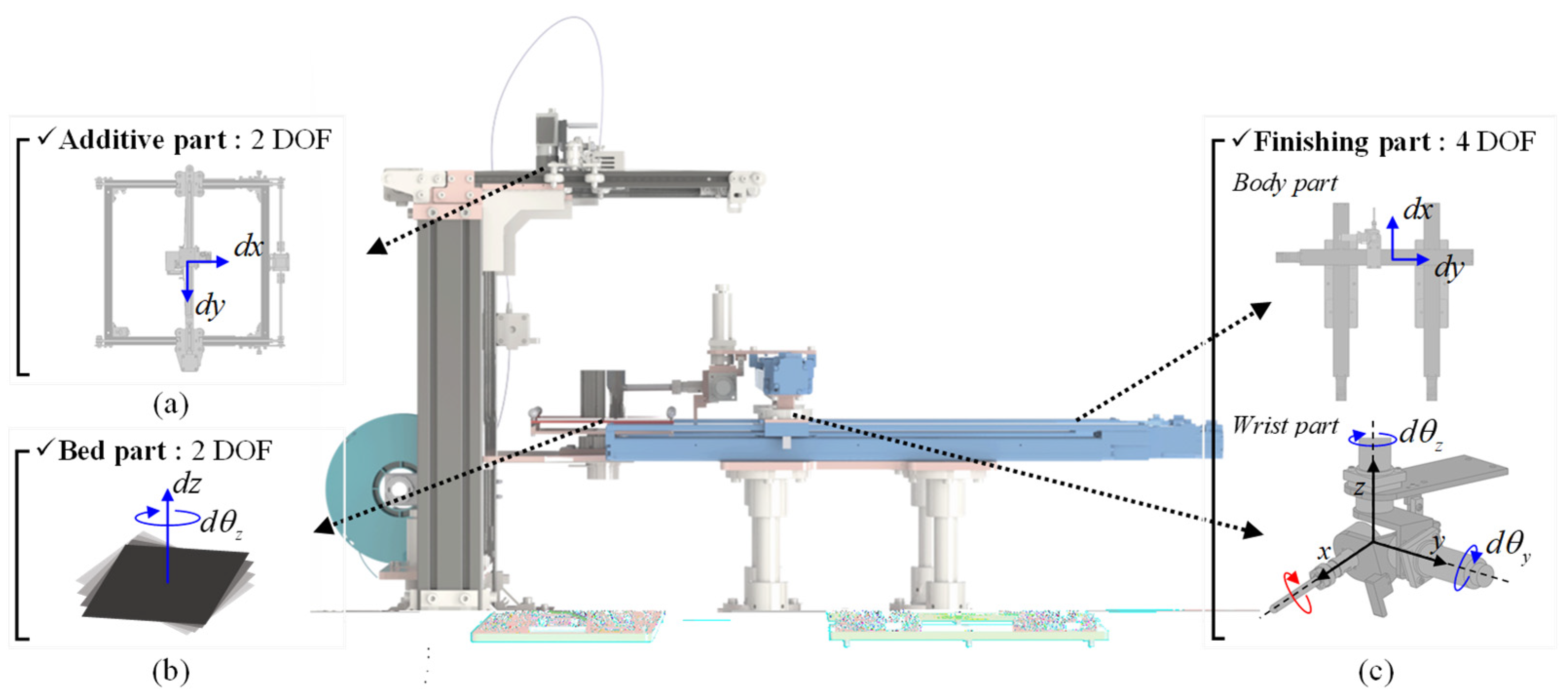
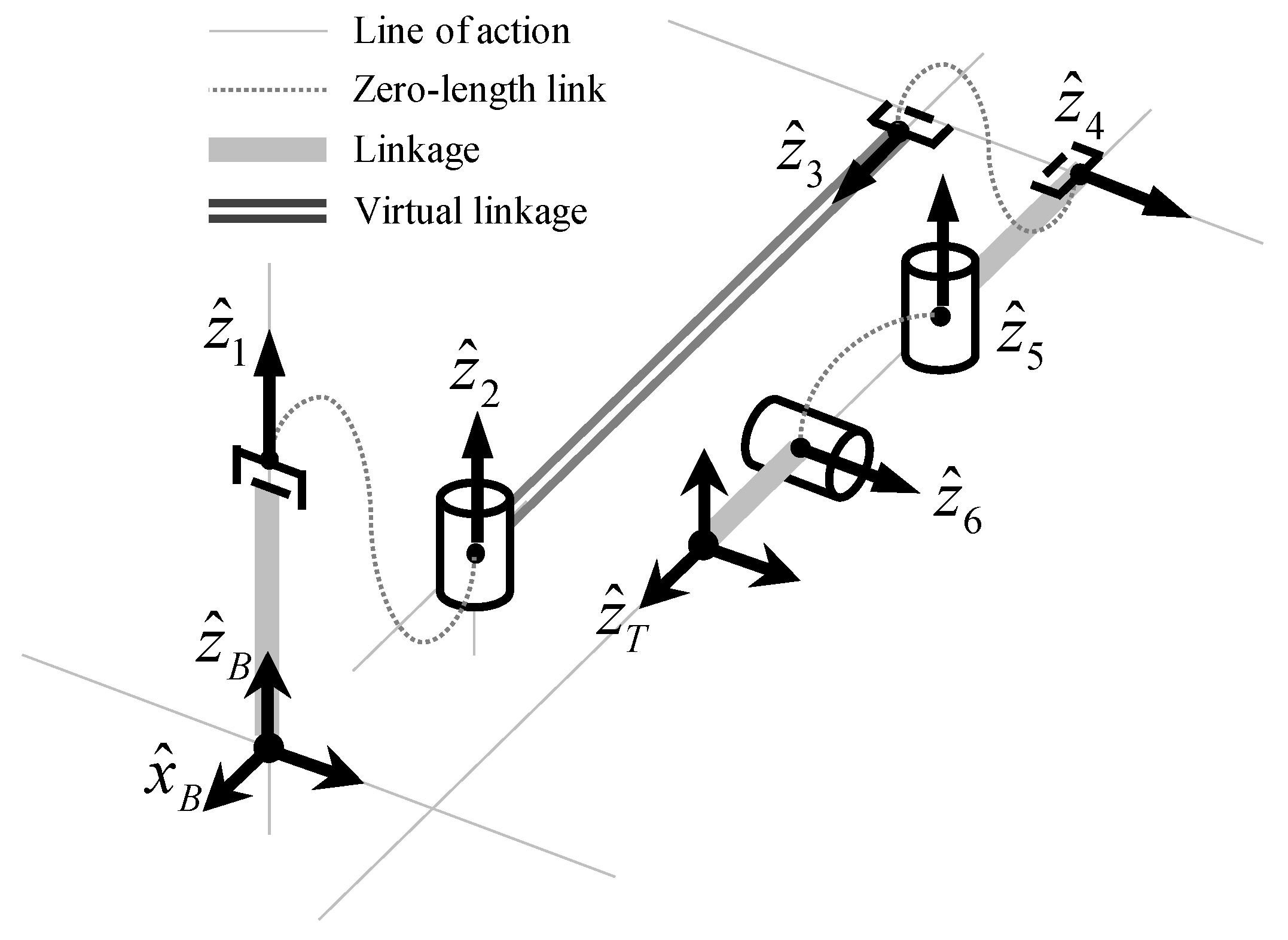
2. Design of AFM and Kinematics Analysis

Figure 1 below illustrates the overall configuration of the AFM, including the AS, FS, and BS. The research motivation of this study comes from an inevitable one-sided layout of an FS with respect to the AS in the AFM. Those two stages share a BS in the AS, and the FS can lightly shave off the rough-surfaced 3D print on the bed. Since the FS that is located at the side of the AS cannot reach all the target points of the 3D print, the bed should be able to rotate the 3D print about the z-axis and translate it in the z-direction. As a result, the AS has 4-dof joints for 3P and 1R during the additive process with AS-BS, and FS has 4-dof and 2-dof integrated joints for 2P2R and 1P1R during the finishing process with FS-BS, respectively. By integrating the physically separated AS, FS, and BS, the proposed AFM can produce a 3D print of dimensions of 180 × 180 × 400 mm³ and lightly finish the 3D print’s rough surface.

The kinematic schematic of the FS-BS is depicted in Figure 2, and the virtual linkage L₃, which is defined to connect the origins of frame {2} and frame {4}, is considered to kinematically join the FS and BS, since both the FS and BS are physically separated. Based on this integrated joint configuration of FS-BS, the product of the exponentials (PoEs) formula is used to derive the forward kinematics. The PoE formula uses an exponential map of twist to represent the instantaneous motion of a rigid body based on its home pose. Thus, let us first choose a fixed stationary frame {s} with the origin located at the plane where the AS and BS lie.

Here, we define M ∈ SE(3) as the home pose of {b} when all joint angles are set to zero. As shown in Figure 2, the tool frame’s origin in its home pose frame is right after the homing process. The subject keeps their elbows facing towards the back and the inside of the forearm facing in the walking or heading direction after the attentive posture. Then, the M can be defined as follows:

$$M=\left[\begin{array}{cccc}-1& 0& 0& L_3-L_e\\ 0& -1& 0& 0\\ 0& 0& 1& 0\\ 0& 0& 0& 1\end{array}\right]$$

(1)

With the manner of the PoE formula defined in Definitions A1–A3, we can write its forward kinematics for arbitrary joint values as a subsequent product of matrix exponentials of Equation (2), each corresponding to a screw motion.

$$T_{BT}\left(\theta \right)=e^{\left[S_1\right]{\theta }_1}{e}^{\left[S_2\right]{\theta }_2}{e}^{\left[S_3\right]{\theta }_3}{e}^{\left[S_4\right]{\theta }_4}{e}^{\left[S_5\right]{\theta }_5}{e}^{\left[S_6\right]{\theta }_6}M$$

(2)

where the ith joint variable θ_i denotes the travel distance along the screw axis. For a revolute joint, ${\omega }_i\in {\mathbb{R}}^3$ can be defined as a unit vector in the positive direction of the joint axis, and $v_i=-{\omega }_i\times q_i$ with any arbitrary point on ith joint axis as written with respect to the fixed base frame {s}. For a prismatic joint, ${\omega }_i=0, v_i\in {\mathbb{R}}^3$ is a unit vector in the direction of positive translation. Therefore, the screw parameters of FS-BS proposed in this study are as shown in

Table 1. The values of the screw parameters $S_i=\left({\omega }_i,v_i\right)$ of FS-BS.

Frame i	$${\mathit{\omega }}_{\mathit{i}}$$	$${\mathit{q}}_{\mathit{i}}$$	$${\mathit{v}}_{\mathit{i}}=-{\mathit{\omega }}_{\mathit{i}}\times {\mathit{q}}_{\mathit{i}}$$
1	(0, 0, 0)	(0, 0, 0)	(0, 0, 1)
2	(0, 0, 1)	(0, 0, 0)	(0, 0, 0)
3	(0, 0, 0)	(−L3, 0, 0)	(1, 0, 0)
4	(0, 0, 0)	(−L3, 0, 0)	(0, 1, 0)
5	(0, 0, 1)	(−L3, 0, 0)	(0, L3, 0)
6	(0, 1, 0)	(−L3, 0, 0)	(0, 0, −L3)

.

3. Redundancy Optimization for Joint Path Planning

3.1. Minimum Euclidian Norm Solution for Optimal Joint Space Solution for Given Tool Path

In general, when we refer to the joint space variable as $\theta \in {\mathbb{R}}^n$ and the cartesian space variable as $X\in {\mathbb{R}}^m$, the kinematic relationship between the joint space variable and the cartesian space variable can be expressed by $X=f\left(\theta \right)$, which is known as forward kinematics. Here, X can be considered a tool pose in this study, and solving to find the joint configuration of the given tool pose becomes inverse kinematics. Conventionally, the joint space of a machining stage consists of five degrees of freedom, while the FS-BS integrated stage in this study has six degrees of freedom in its joint space. Consequently, since the number of joints n is larger than the dimension of the given tool pose, m, the kinematics $X=f\left(\theta \right)$ become an underdetermined problem. Differential kinematics is derived through linearization, as shown in Equation (3), for the non-linear kinematic model to find the optimal joint space configuration for a given tool pose.

$$\dot{X}=J^{+}\left(\theta \right)\cdot \dot{\theta }$$

(3)

where $J\left(\theta \right)\triangleq \frac{\partial f}{\partial \theta }\in {\mathbb{R}}^{m\times n}$ is the Jacobian matrix of the manipulation variable. $\dot{\theta }\in {\mathbb{R}}^n$ represents the instantaneous joint rate, $\dot{ X}\in {\mathbb{R}}^m$ is the instantaneous tool’s spatial velocity, and $J^{+}\left(\theta \right)\in {\mathbb{R}}^{n\times m}$ is the pseudoinverse of $J\left(\theta \right)$, signifying the inverse of the Jacobian. The general solution is obtained using the following optimization objectives with the pseudoinverse of the Jacobian matrix as follows [18,19,20]:

$$\mathrm{argmin}‖\dot{\theta }-J^{+}\left(\theta \right)\dot{X}+\left(I_n-J^{+}\left(\theta \right)J\left(\theta \right)\right)z‖$$

(4)

where $z\in {\mathbb{R}}^n$ is an arbitrary vector, and $I_n\in {\mathbb{R}}^{n\times n},$ which is used to ensure proper dimensionality in the equation, indicates an identity matrix. If the exact solution does not exist, Equation (4) covers all the least-squares solutions that minimize $‖\dot{\theta }-J^{+}\left(\theta \right)\dot{X}+\left(I_n-J^{+}\left(\theta \right)J\left(\theta \right)\right)z‖$, which means the absolute difference between the required tool’s spatial velocity and the generated tool’s spatial velocity when solving Equation (5). The second term $\left(I_n-J^{+}\left(\theta \right)J\left(\theta \right)\right)z$ accounts for the null space motion that does not affect the end-effector velocity. $\left(I_n-J^{+}\left(\theta \right)J\left(\theta \right)\right)$ is often referred to as the null space projection matrix, and it projects any motion that is not directly contributing to the desired end-effector velocity onto the null space. When you multiply this matrix by the vector z, it ensures that the additional joint motion does not affect the end-effector velocity.

$$\mathrm{argmin}‖\dot{\theta }-J^{+}\left(\theta \right)\dot{X}‖$$

(5)

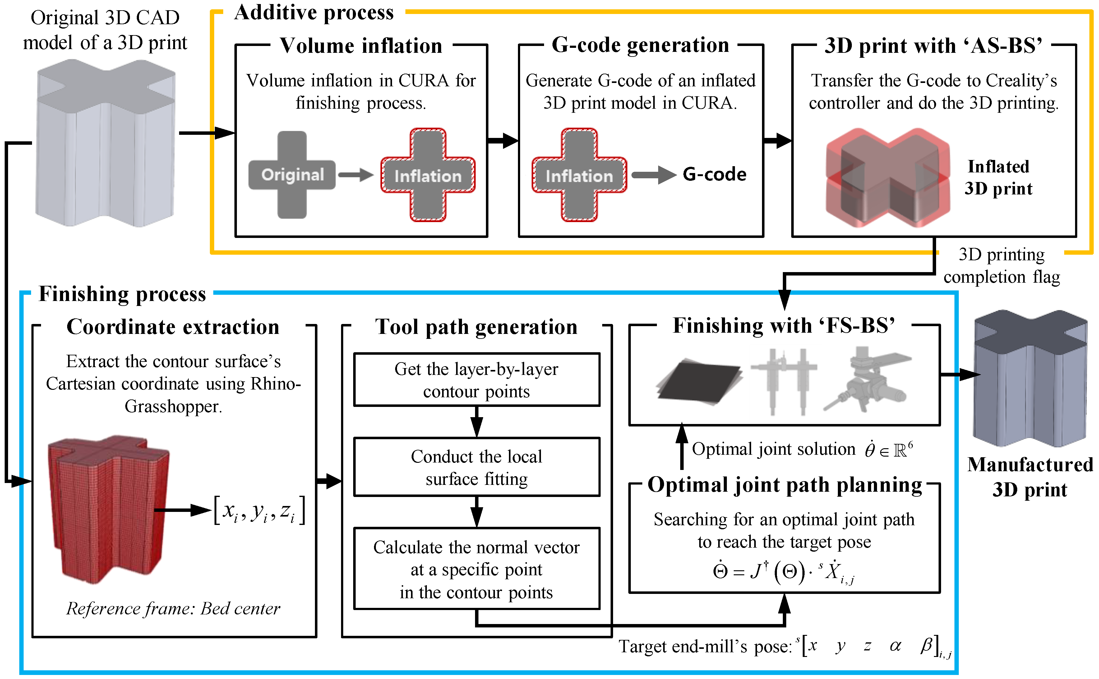
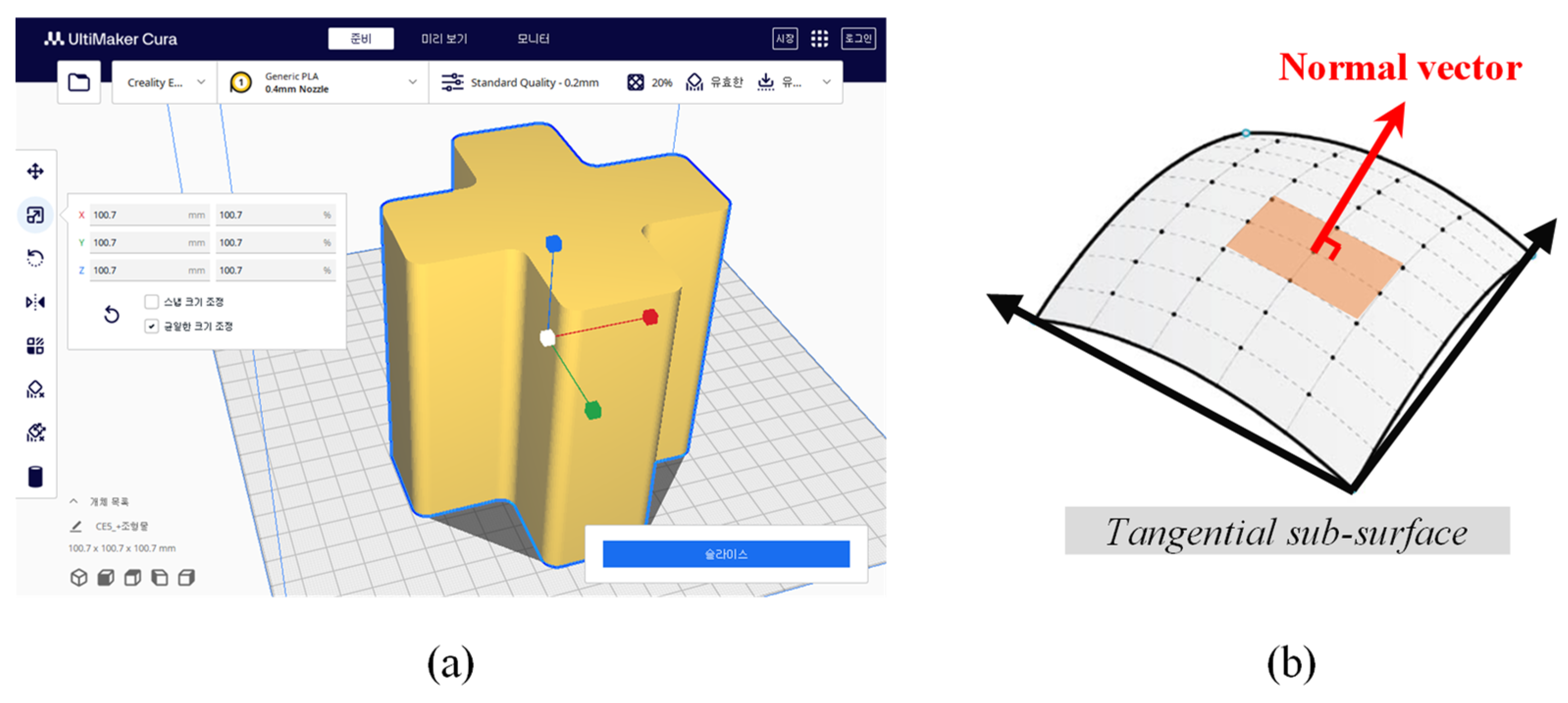
3.2. Tool Path Generation of the Inflated CAD Model of 3D Print with CURA Slicer

Before finishing, the additive process should be performed, considering the depth of cut in the finishing of the 3D print (Figure 3). In a Cura slicer [21], uniform scaling refers to the process of scaling a 3D model uniformly in all dimensions (X, Y, and Z axes) by the same factor. This means that the object is resized proportionally without altering its shape or aspect ratio. As shown in Figure 4, the scaling factor can be specified by entering specific scaling percentages or dimensions. According to the results of our previous research [22], which has investigated the relationship between the additive and machining process conditions, it has been confirmed that the satisfactory scaling percentage is approximately 70% of the nozzle diameter. Thus, in the case of a 1 mm nozzle diameter, a conventional size, the scaling percentage for 0.7 mm should be calculated considering the volume of 3D prints. For instance, in the case of a 100 × 100 × 100 mm³ object, it will be produced with dimensions of 100.7 mm in the x and y axes.

Now, to obtain the layer-by-layer tool path for the finishing process, the layer-by-layer boundary of the scaled 3D CAD model is obtained with Rhino’s Grasshopper 3D [23], and the tool pose at a specific point on the boundary is calculated with the Local Surface Fitting (LSF) method shown in Algorithm 1. The complete tool path in the Cartesian space can be generated as a result of calculating the tool orientation with the LSF and considering the depth of cut of 0.7 mm into the direction of tool orientation.

Algorithm 1 Tool path generation
1:	Input (3D point surface coordinate Ni(xi,yi,zi))
2:	for i = 1 to n do
3:	if  $N_i\left(2\right)==i$, then
4:	for j = 1 to n do
5:	layer_points_x = Nj(0)
6:	layer_points_y = Nj(1)
7:	end
8:	surface_spline = RectBivariateSpline(layer_points_x, layer_points_y, $N_i$)
9:	z_point = surface_spline(x, y, grid=False)
10:	Calculate
11:	dx = surface_spline(x, y, dx = 1, dy = 0, grid = False)
12:	dy = surface_spline(x, y, dx = 0, dy = 1, grid = False)
13:	normal_vector$/=‖\left[-dx,-dy, 1\right]‖$
14:	return  normal_vector
15:	end

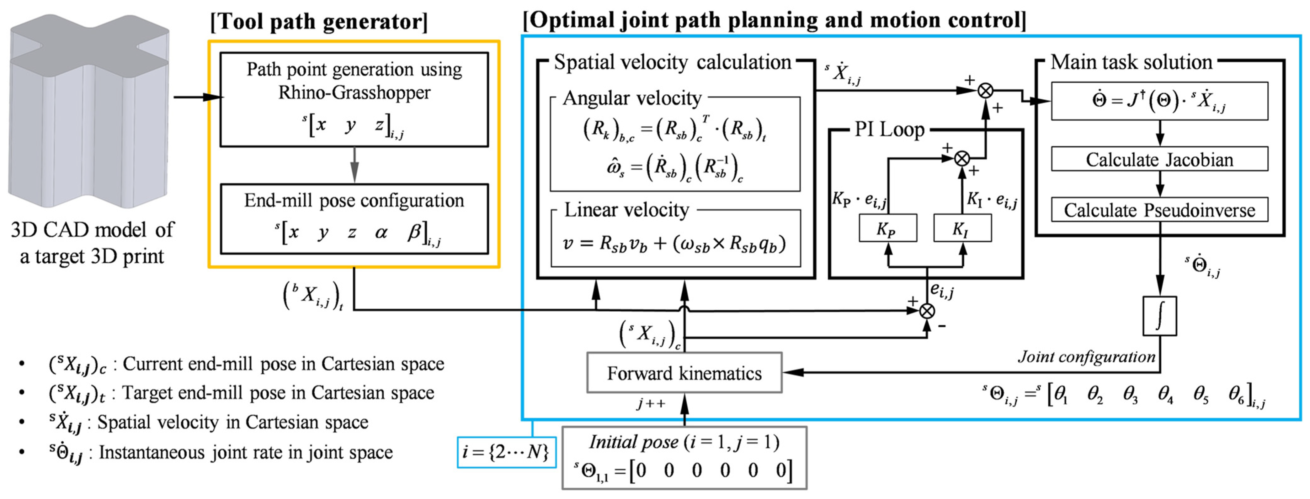
3.3. Frameworks of Optimal Joint Path Planning and Motion Control

Figure 5 illustrates the block diagram for the optimal joint path planning and motion control discussed in this paper. Local optimal joint path planning aims to follow the target pose defined along the given path from the tool path generator. It is based on differentiation, as shown in Equation (5). This approach uses the differential kinematics at the current joint configuration to find an optimal solution in the joint velocity space. The control input for motion control is a combination of the target pose for the next step and the output of the PI controller, designed to compensate for the error from the previous step. This combination, through Equation (5), generates the optimal joint velocity to accurately follow the final target pose. In this study, the gain values of the PI controller were experimentally set to k_p = 3.5 and k_i = 0.2, respectively.

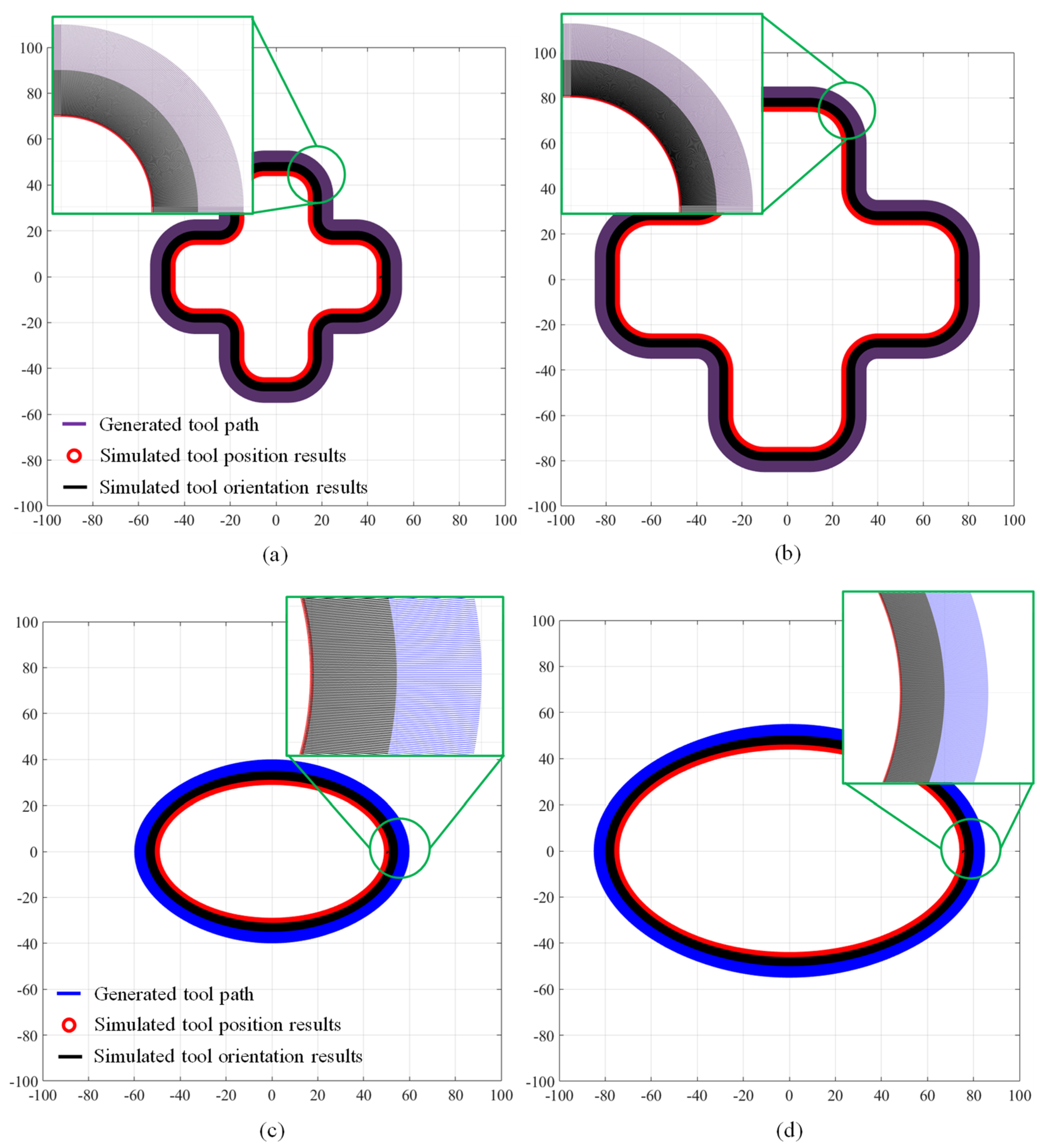
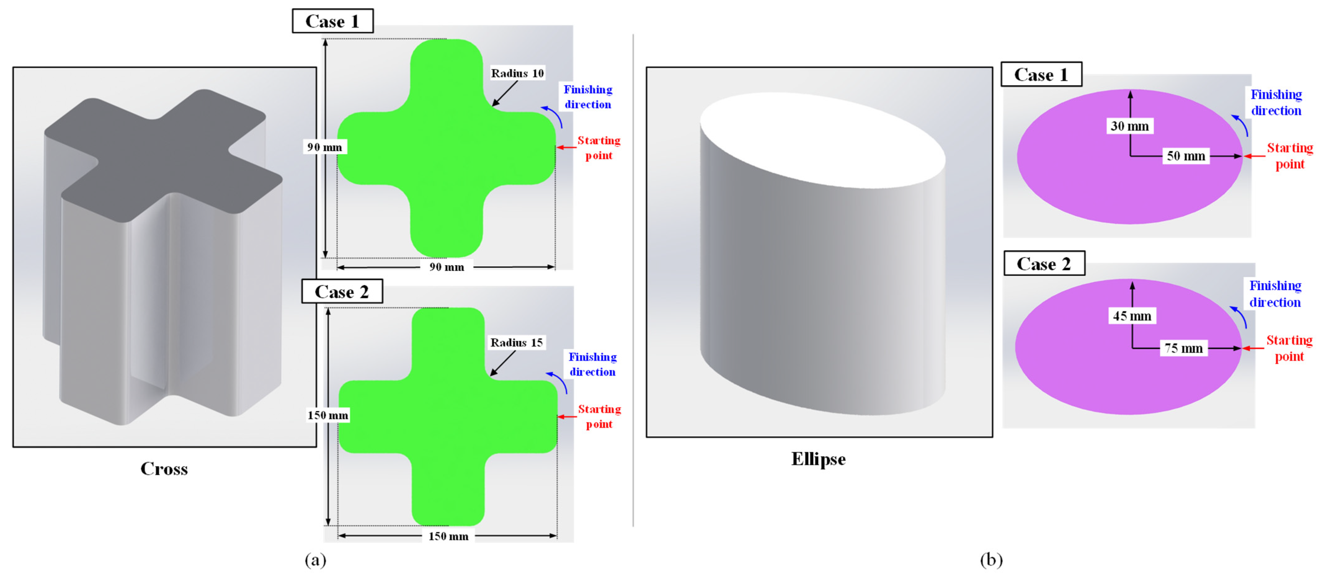
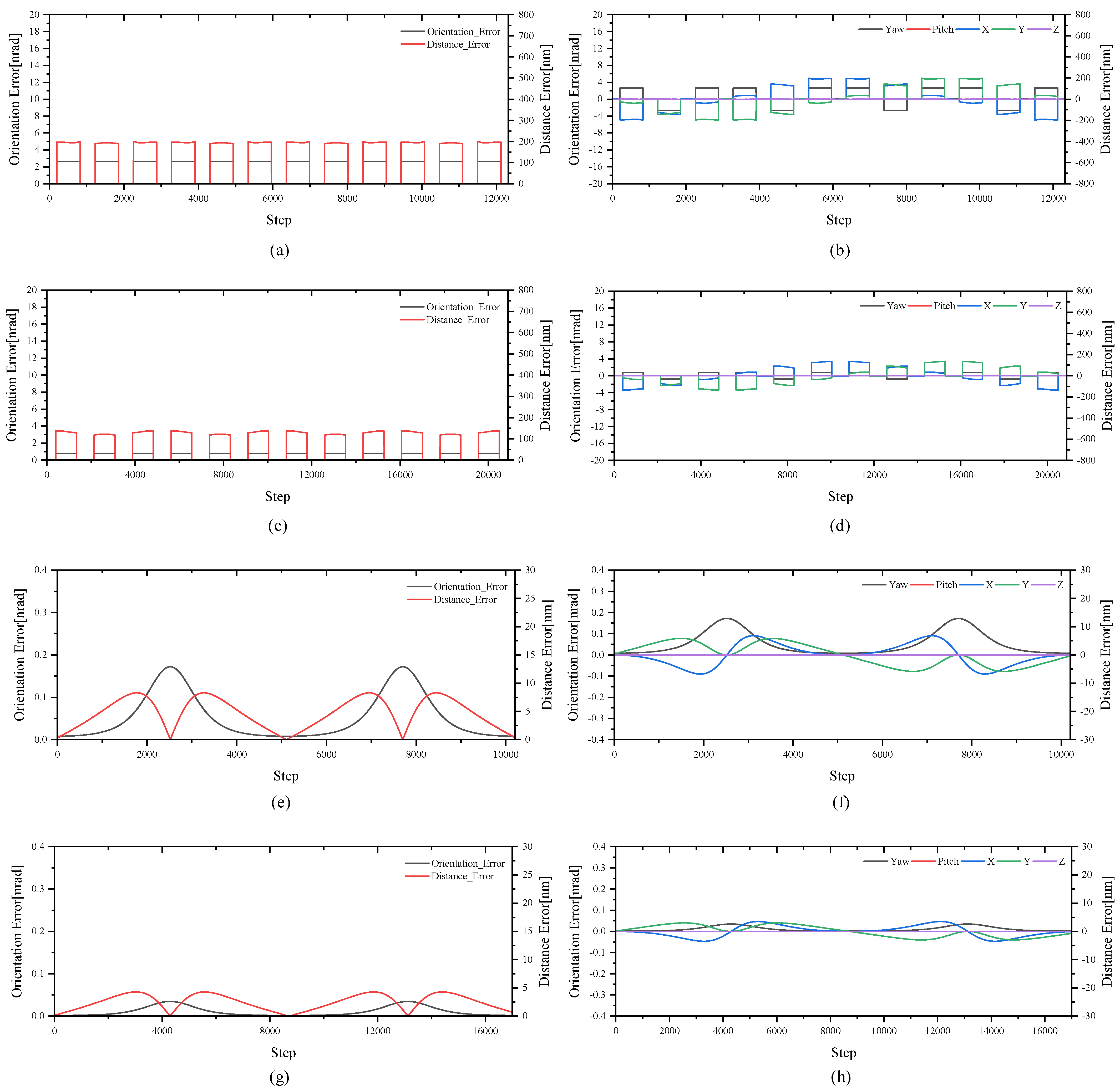
4. Results and Conclusions

This section conducts a numerical analysis of a 3D-printed CAD model with the geometric shapes depicted in Figure 6 to verify the numerical accuracy of the optimal joint path planning algorithm proposed for FS-BS. Figure 6a represents a cylindrical structure with a cross-sectional shape consisting of straight and curved segments. Figure 6b illustrates a cylindrical structure with an elliptical cross-sectional shape exhibiting continuous curvature variation. Two cases were distinguished to evaluate the numerical accuracies of the optimal joint path planning based on the design parameters of the respective 3D print’s model: case-1 and case-2. In Figure 6a of the cross-shape, case-1 is designed with dimensions of 90 mm width and 90 mm height and a curved segment with a rotation radius of 10 mm. In comparison, case 2, which has an oversized area of 1.5 times that of case 1, comprises dimensions of 150 mm width, 150 mm height, and a curved segment rotation radius of 15 mm. For Figure 6b of the ellipse-shape, case-1 has major and minor axes of 50 mm and 35 mm, respectively, while case-2, oversized by 1.5 times compared to case-1, possesses major and minor axes of 75 mm and 45 mm, respectively. The analysis conditions for both test models start from the top-right center as the starting point, following a counterclockwise direction, as depicted in Figure 6. Interpolation was performed to achieve an incremental point-to-point displacement at approximately 0.025 mm.

Figure 7 illustrates the tool path generated through the algorithm presented in Algorithm 1 and represents the tool pose obtained via optimal joint path planning. Notably, there is a minimal discrepancy between the desired tool pose on the tool path and the one obtained through optimal joint path planning. This fact is corroborated by the pose error plots in Figure 8 and the RMS error results presented in

Table 2. RMS and peak value of orientation error and distance error for each test shape and case.

	Case 1		Case 2
	Distance Error [RMS (Peak)]	Orientation Error [RMS (Peak)]	Distance Error [RMS (Peak)]	Orientation Error [RMS (Peak)]
Cross shape	152.33 (201.00) × 10−9 m	2.04 (2.62) × 10−9 rad	95.49 (137.62) × 10−9 m	0.57 (0.77) × 10−9 rad
Ellipse shape	5.38 (8.29) × 10−9 m	0.07 (0.17) × 10−9 rad	2.78 (4.27) × 10−9 m	0.01 (0.03) × 10−9 rad

. In Table 2, the RMSE (Root Mean Square Error) for the distance in the cases of the cross shape, namely, case 1 and case 2, are 152.33 nm and 95.49 nm, respectively. This indicates a reduction of approximately 37% in case 2 compared with case 1. Similarly, the orientation RMSE values for case 1 and case 2 are 2.04 nrad and 0.57 nrad, respectively, depicting a reduction of roughly 72% in case 2 compared with case 1.

The reduced error in case 2 compared to case 1 can be attributed to most errors occurring in curved segments, as is evident in Figure 8a–d. As the radius of rotation (R) increases, there are more target points, resulting in smoother changes in the endmill’s orientation. Additionally, in the case of the cross shape, it can be observed that the error is amplified at 12 points. This amplification occurs at the edge sections. In the case of straight lines, the error is almost zero because only the x and y-axis translations of the FS appear. However, in the case of curves, the centers of the 12-edge radii are offset from the center of the bed rotation part. Therefore, when creating a path to align the endmill’s orientation perpendicular to the 3D print surface, it is necessary to rotate the BS and perform simultaneous x, y translations of the FS and rapid yawing. This is thought to lead to the amplification of the error. For the ellipse shape (Figure 8e–h), the errors are notably more minor compared to the cross shape, with distance and orientation errors approaching zero at the midpoint and exhibiting a symmetrical pattern. This can be attributed to the nature of the ellipse shape, where there are fewer drastic changes in the endmill’s pose due to the alternating straight and curved sections, resulting in more minor errors than for the cross shape. Moreover, the symmetrical characteristic of the ellipse shape leads to errors nearing zero at the midpoint, indicating similar poses between the starting point and the endmill. Furthermore, as in Table 2, the distance RMSE for case 1 and case 2 in the ellipse shape is 5.38 nm and 2.78 nm, respectively, showcasing a reduction of about 48% in case 2 compared with case 1. Similarly, the orientation RMSE values for case 1 and case 2 are 0.07 nrad and 0.01 nrad, respectively, indicating a reduction of approximately 86% in case 2 compared with case 1. Similar to the cross shape, this reduction in error in case 2 is due to its smoother curvature, resulting in fewer variations in the endmill’s orientation.

Consequently, the optimal joint path planning algorithm developed in this paper exhibits maximum distance and orientation errors of 201 nm and 2.62 nrad, respectively. With both the distance and orientation RMSE values—153 nm and 2.05 nrad, respectively—being smaller than ±10 μm and 20 μm, the precision of the tool path generation and general machining accuracy outlined in this paper fully meets industry requirements.

References

1. Kumbhar, N.N.; Mulay, A.V. Post processing methods used to improve surface finish of products which are manufactured by additive manufacturing technologies: A review. J. Inst. Eng. India Ser. C 2018, 99, 481–487. [Google Scholar] [CrossRef]
2. Jiang, P.; Rifat, M.; Basu, S. Impact of surface roughness and porosity on lattice structures fabricated by additive manufacturing-A computational study. Procedia Manuf. 2020, 48, 781–789. [Google Scholar] [CrossRef]
3. Grzesik, W. Hybrid additive and subtractive manufacturing processes and systems: A review. J. Mach. Eng. 2018, 18, 5–24. [Google Scholar] [CrossRef]
4. Grzesik, W. Hybrid manufacturing of metallic parts integrated additive and subtractive processes. Mechanik 2018, 9, 468–475. [Google Scholar] [CrossRef]
5. DMG MORI. Lasertec 65 DED Hybrid. DMG MORI. Available online: https://de.dmgmori.com/produkte/maschinen/additive-manufacturing/pulverdueseverfahren/lasertec-65-ded-hybrid (accessed on 1 January 2016).
6. Ma, G.; Zhao, G.; Li, Z.; Yang, M.; Xiao, W. Optimization strategies for robotic additive and subtractive manufacturing of large and high thin-walled aluminum structures. Int. J. Adv. Manuf. Technol. 2019, 101, 1275–1292. [Google Scholar] [CrossRef]
7. Zhang, S.; Gong, M.; Zeng, X.; Gao, M. Residual stress and tensile anisotropy of hybrid wire arc additive-milling subtractive manufacturing. J. Mater. Process. Technol. 2021, 293, 117077. [Google Scholar] [CrossRef]
8. Singh, R.; Singh, S.; Singh, I.P.; Fabbrocino, F.; Fraternali, F. Investigation for surface finish improvement of FDM parts by vapor smoothing process. Compos. Part B Eng. 2017, 111, 228–234. [Google Scholar] [CrossRef]
9. Cunico, M.W.M.; Cavalheiro, P.M.; de Carvalho, J. Development of automatic smoothing station based on solvent vapour attack for low cost 3D Printers. In 2017 International Solid Freeform Fabrication Symposium; University of Texas at Austin: Austin, TX, USA, 2017. [Google Scholar]
10. Tomal, A.N.M.A.; Saleh, T.; Khan, R. Improvement of dimensional accuracy of 3-D printed parts using an additive/subtractive based hybrid prototyping approach. IOP Conf. Ser. Mater. Sci. Eng. 2017, 260, 012031. [Google Scholar] [CrossRef]
11. Lu, Y.-A.; Tang, K.; Wang, C.-Y. Collision-free and smooth joint motion planning for six-axis industrial robots by redundancy optimization. Robot. Comput.-Integr. Manuf. 2021, 68, 102091. [Google Scholar] [CrossRef]
12. Liu, Z.; Li, R.; Zhao, L.; Xia, Y.; Qin, Z.; Zhu, K. Automatic joint motion planning of 9-DOF robot based on redundancy optimization for wheel hub polishing. Robot. Comput.-Integr. Manuf. 2023, 81, 102500. [Google Scholar] [CrossRef]
13. Dai, C.; Lefebvre, S.; Yu, K.-M.; Geraedts, J.M.P.; Wang, C.C.L. Planning jerk-optimized trajectory with discrete time constraints for redundant robots. IEEE Trans. Autom. Sci. Eng. 2020, 17, 1711–1724. [Google Scholar] [CrossRef]
14. Lu, S.; Ding, B.; Li, Y. Minimum-jerk trajectory planning pertaining to a translational 3-degree-of-freedom parallel manipulator through piecewise quintic polynomials interpolation. Adv. Mech. Eng. 2020, 12, 1687814020913667. [Google Scholar] [CrossRef]
15. Gosselin, C.; Schreiber, L.-T. Kinematically redundant spatial parallel mechanisms for singularity avoidance and large orientational workspace. IEEE Trans. Robot. 2016, 32, 286–300. [Google Scholar] [CrossRef]
16. Tong, J.; Lou, Y.; Lyu, H.; Liu, Y.; Yang, X. Automatic Tool Path Planning Strategy Based on Feature Extraction of 3D Models. In Proceedings of the 2018 IEEE International Conference on Robotics and Biomimetics (ROBIO), Kuala Lumpur, Malaysia, 12–15 December 2018; pp. 1677–1682. [Google Scholar]
17. Verl, A.; Valente, A.; Melkote, S.; Brecher, C.; Ozturk, E.; Tunc, L.T. Robots in machining. CIRP Ann. 2019, 68, 799–822. [Google Scholar] [CrossRef]
18. Huber, G.; Wollherr, D. Globally Optimal Online Redundancy Resolution for Serial 7-DOF Kinematics along SE (3) Trajectories. In Proceedings of the 2021 IEEE International Conference on Robotics and Automation (ICRA), Xi’an, China, 30 May–5 June 2021; pp. 7570–7576. [Google Scholar]
19. Nakamura, Y. Advanced Robotics: Redundancy and Optimization; Addison-Wesley Longman Publishing Co., Inc.: Reading, MA, USA, 1990. [Google Scholar]
20. Wang, J.; Li, Y.; Zhao, X. Inverse kinematics and control of a 7-DOF redundant manipulator based on the closed-loop algorithm. Int. J. Adv. Robot. Syst. 2010, 7, 37. [Google Scholar] [CrossRef]
21. Ultimaker. Ultimaker/Cura: Open Source 3D Printer Management Software. 2023. Available online: https://github.com/Ultimaker/Cura (accessed on 22 November 2023).
22. Yu, J.W.; Hyung, J.J.; Park, J.H.; Dong, H.L. Analysis of Correlation between FDM Additive and Finishing Process Conditions in FDM Additive-Finishing Integrated Process for the Improved Surface Quality of FDM Prints. J. Korean Soc. Precis. Eng. 2022, 39, 159–165. [Google Scholar] [CrossRef]
23. Grasshopper 3D. Version Rhino8. 2023. Available online: https://www.rhino3d.com/download/ (accessed on 22 November 2023).
Figure 1. Overview of the AFM, including AS, FS, and BS, with descriptions of joint motions in each module. (a) Additive part, (b) Bed part, (c) Finishing part.
Mathematics 11 04995 g001
Figure 2. Kinematic schematic of FS-BS composed of 2P2R (right, FS) and 1P1R (left, BS), connected through virtual linkage L3.
Mathematics 11 04995 g002
Figure 3. The overall framework of additive process and finishing process.
Mathematics 11 04995 g003
Figure 4. (a) Specification of scaling factor in the CURA slicer, (b) schematic diagram of determining tool orientation and tool path.
Mathematics 11 04995 g004
Figure 5. The overall framework of optimal joint path planning and motion control algorithm.
Mathematics 11 04995 g005
Figure 6. Geometric descriptions of two test models: (a) two cases of the cross shape and (b) two cases of the ellipse shape.
Mathematics 11 04995 g006
Figure 7. Results of the numerical analysis of the optimal joint path planning: (a) case 1 of the cross shape, (b) case 2 of the cross shape, (c) case 1 of the ellipse shape, (d) case 2 of the ellipse shape.
Mathematics 11 04995 g007
Figure 8. Orientation error and distance error for each test shape and case (a) error magnitude: case 1 of cross shape, (b) error value for each pose element: case 1 of cross shape, (c) error magnitude: case 2 of cross shape, (d) error value for each pose element: case 2 of cross shape, (e) error magnitude: case 1 of ellipse shape, (f) error value for each pose element: case 1 of ellipse shape, (g) error magnitude: case 2 of ellipse shape, (h) error value for each pose element: case 2 of ellipse shape.
Mathematics 11 04995 g008