Article

Multiple Control Policy in Unreliable Two-Phase Bulk Queueing System with Active Bernoulli Feedback and Vacation

1
Department of Mathematics, Vel Tech Rangarajan Dr. Sagunthala R&D Institute of Science and Technology, Chennai 600062, India
2
Department of Control Systems and Instrumentation, Faculty of Mechanical Engineering, VSB-Technical University of Ostrava, 17, Listopadu 2172/15, 70800 Ostrava, Czech Republic
3
Department of Mechanical Engineering, Vel Tech Rangarajan Dr. Sagunthala R&D Institute of Science and Technology, Chennai 600062, India
*
Author to whom correspondence should be addressed.
Mathematics 2024, 12(1), 75; https://doi.org/10.3390/math12010075
Submission received: 27 October 2023 / Revised: 10 December 2023 / Accepted: 19 December 2023 / Published: 25 December 2023

Abstract

:
In this paper, a bulk arrival and two-phase bulk service with active Bernoulli feedback, vacation, and breakdown is considered. The server provides service in two phases as mandatory according to the general bulk service rule, with minimum bulk size a and maximum bulk size b . In the first essential service (FES) completion epoch, if the server fails, with probability δ , then the renewal of the service station is considered. On the other hand, if there is no server failure, with a probability 1 δ , then the server switches to a second essential service (SES) in succession. A customer who requires further service as feedback is given priority, and they join the head of the queue with probability β . On the contrary, a customer who does not require feedback leaves the system with a probability 1 β . If the queue length is less than a after SES, the server may leave for a single vacation with probability 1 β . When the server finds an inadequate number of customers in the queue after vacation completion, the server becomes dormant. After vacation completion, the server requires some time to start service, which is attained by including setup time. The setup time is initiated only when the queue length is at least a . Even after setup time completion, the service process begins only with a queue length ‘N’ (N > b). The novelty of this paper is that it introduces an essential two-phase bulk service, immediate Bernoulli feedback for customers, and renewal service time of the first essential service for the bulk arrival and bulk service queueing model. We aim to develop a model that investigates the probability-generating function of the queue size at any time. Additionally, we analyzed various performance characteristics using numerical examples to demonstrate the model’s effectiveness. An optimum cost analysis was also carried out to minimize the total average cost with appropriate practical applications in existing data transmission and data processing in LTE-A networks using the DRX mechanism.
MSC:
60K25; 68M20; 90B22

1. Introduction

Several academicians have tested queue systems with vacations and their numerous combos. Some of those studies are queue structures with vacation queue fashions via Tian and Zhang [1]. In many actual applications, there can be a couple of arrivals into the machine. These types of systems are labeled as bulk arrival queue structures. For bulk carrier queue structures with multiple vacations, Arumuganathan and Jeyakumar obtained consistent national conditions for numerous performance measures and value optimization [2]. Jeyakumar and Senthilnathan recently obtained the steady-state queue size distribution for the MX/G (a, b)/1 queue system with multiple vacations [3]. In all queue models with vacations that have been studied in this context, the server remains on vacation, even whilst the queue period is excessive enough to initiate the primary provider. The modeling of actual-time systems can benefit from those vacation methods. Baba examined the M/PH/1 line with working vacations and interruptions [4]. The MX/G (a, b)/1 queue model with vacation interruption was also researched by Haridass and Arumuganathan [5]. Through real-time applications, they deduced diverse queue device functions. Gao and Liu investigated the M/G/1 queue under a Bernoulli agenda with a single working vacation and vacation interruption [6]. Customers arrive at a queue served by a single server, and their arrivals follow a Poisson process. The duration of the service provided by the server conforms to an exponential distribution. However, the server takes periodic vacations which are scheduled based on a Bernoulli process. During the vacations, the server can be interrupted and resume service if a customer arrives, preventing the vacation from being completed, as studied by Tao et al. [7]. A countless-buffer bulk arrival queue with a bulk-size-dependent provider was tested by Pradhan and Gupta [8]. Madan et al. studied the consistent state of two MX/M (a, b)/1 queue models with random breakdowns. In 2003, they took into account the reality that the repair time is deterministic for one version and exponential for every other. It has been cited in the literature on queue fashions with server breakdown that, excluding Madan et al., each creator who discusses server breakdown in the context of a bulk provider queue version deals with a server that can only serve one customer at a time. The server may also interrupt right away if trouble arises. Yet, in the majority of instances, it is impossible to disturb the server before it has completed providing its bulk services [9]. Jeyakumar and Senthilnathan also studied breakdown without carrier disruption in a bulk carrier queue model and a bulk arrival queue model. They developed a model using closedown time and constructed probability-generating functions for the completion epochs of services, vacations, and renewals [10]. Wu et al. investigated an M/G/1 queue system with an N-policy, a solitary vacation, an unreliable service station, and a replaceable repair facility [11,12].
Hanumantha Rao Sama et al. introduced an unstable server and delayed repair for a bulk arrival Markovian queueing system with state-dependent arrival and an N-policy [13]. Ankamma Rao et al. examined a two-phase queueing model, denoted M/M/1, incorporating server startup, time-out, and breakdowns [14]. Samuel U. Enogwe et al. investigated a non-Markovian queueing system that incorporates two distinct types of service mechanisms: balking and Bernoulli server vacation. The model is referred to as a bivariate Markov process and includes the elapsed service time and vacation time as supplementary variables [15]. GnanaSekar and Indhira Kandaiyan delved into the dynamics of a retrial queueing system with distinctive features, including delayed repair, a feedback mechanism, and the incorporation of a working vacation policy, as outlined in their article. If the essential and sufficient requirements are viable, the system can be stabilized [16]. Server breakdown based on service modes was introduced by Niranjan. In this paper, the author used supplementary variable techniques to derive important performance measures [17]. Blondia analyzed energy harvesting in the queueing model for a wireless sensor node [18]. C.K. Deena Merit and Haridass worked on a simulation analysis of the bulk queueing system with a working breakdown [19]. An application of a queueing system in 4G/5G networks was presented by V. Deepa et al. [20]. Niranjan et al. introduced two types of breakdown with two phases of service in bulk queueing systems [21]. In this study, we examine an MX/G (a, b)/1 queuing system with an optional additional service and numerous vacations, and setup time is examined by Ayyappan and Deepa [22]. Niranjan et al. analyzed a non-Markovian bulk queueing system with renewal and startup/shutdown times [23]. Nithya and Haridass conducted a maximum entropy analysis of a queueing system that controls both arrival and bulk service, incorporating breakdowns and multiple vacation periods [24]. In their article, Enogwe and Obiora-Ilouno explored the impacts of three pivotal factors—reneging, server breakdown, and server vacation—on various stages of a queueing system with bulk arrivals and a single server [25]. Khan IE and Paramasivam R analyzed the quality control policy for the Markovian model with feedback, balking, and maintaining reneged clients using an iterative method for the nth customer in the system [26]. Ammar, Rajadurai P analyzed an innovative type of retry queueing system with functional breakdown services presented in this inquiry. Priority and regular clients are two different categories that are taken into consideration [27]. Gabi Hanukov and Shraga Shoval introduce a compelling vacation queue model that accounts for dynamic server service rates affected by factors like human fatigue and machinery wear. The analysis employed multidimensional methods to explore the impact of different vacation policies on system efficiency. The findings underscore the significant positive effect of strategic vacation scheduling on mean customer waiting time, suggesting potential benefits even when switching to a temporary server during times of higher main-server service rates [28]. Xing et al. investigated traffic accident patterns in undersea tunnels, offering valuable insights into the evolution of vehicle congestion queuing. The authors present precise queue-length estimation models based on shockwave theory and real-time data input, demonstrating optimal accuracy with a 30 s time interval. The results highlight the effectiveness of the model, with an accuracy of 92.34% for the maximum queue-length estimation model and 83.50% for the real-time whole-process queue-length estimation model. The proposed approach outperforms the input–output model, indicating its potential for supporting timely and effective control measures in undersea tunnel traffic management [29]. Mohan Chaudhry et al. addresses a finite-space, single-server queueing system with a unique (a, b)-bulk service rule and finite-buffer capacity ‘N’. It introduces a novel approach utilizing embedded Markov chains, Markov renewal theory, and semi-Markov processes to derive probability distributions for queue lengths at post-departure and random epochs. This investigation establishes a functional relationship between the probability-generating function representing the queue-length distribution and the Laplace–Stieltjes transform (LST) of the queueing-time distribution. This connection facilitates the derivation of waiting-time distributions for individual random customers. The use of LSTs facilitates a comprehensive discussion of the probability density function of waiting times, emphasizing numerical implementations for practical applications [30]. Laurentiu Rece et al. introduce a novel approach using queueing theory models to optimize production department size, production costs, and provisioning. This method employs queuing mathematical models to form the basis for an experimental algorithm and a numerical approach. This research effectively employed these models in designing a practical industrial engineering unit, aligning with technological flow and equipment schemes. The focus on minimizing costs in terms of server count is addressed using the Monte Carlo method, showcasing the practicality of iterative methods like Jacobi and Gauss–Seidel in solving the associated linear system for Jackson queueing networks [31]. Mustafa Demircioglu et al. investigated the influence of disasters on a discrete-time single-server queueing system featuring general independent arrivals and service times. Disasters, modeled as a Bernoulli process, lead to the simultaneous removal of all customers. This study employs a two-dimensional Markovian state description, providing expressions for probability-generating functions, and average values, variances, and tail probabilities for both system content and customer sojourn time are analyzed under a first-come-first-served policy. The derivation of customer loss probability due to disaster occurrences is also addressed, with numerical illustrations enhancing the understanding of the proposed models [32]. In all the above queueing models, essential two-phase bulk service is not considered. It is mandatory to analyze many real-time systems such as communication systems, the manufacturing industry, production systems, network systems, etc. Multiple control policies and renewal of service stations in first-phase customer feedback are the technical terms introduced in this paper which will be useful the studying the performance analysis of DRX mechanisms in network systems.
2. Motivation

Long term evolution-advanced (LTE-A) networks are characterized by two critical elements: power saving and quality of service (QoS). ‘Discontinuous reception’ (DRX) is a widely utilized mechanism in mobile communication networks to improve power efficiency. By employing DRX, mobile devices can conserve battery life effectively while maintaining seamless connectivity. This method is crucial in enhancing the overall performance and longevity of mobile devices. The first essential service starts using power saving and LTE. The data signals are passed, the data transfer is authenticated, and the minimum value is 1024 mbps and the maximum 4096 mbps. In LTE-A networks, data transfer between the mobile device and the network is orchestrated through a series of negotiated phases for the user equipment (UE). During the data transfer, sometimes the system may be affected by a virus. The service will not be abruptly interrupted; instead, it will be sustained for the ongoing bulk of data, attached or else transferred by carrying out some technical arrangements. After the service is completed, the antivirus is activated and detects the problems in the system. If there are no issues, the process is continued. In this paper, we propose the development of a novel appliance that adapts its functionality based on the type of traffic being processed by the user equipment (UE).
The second essential service is proposed to switch the DRX mechanism combined with the quality of service, and it helps to check the quantity and quality of data that are going to be transferred. The minimum value is 1000 mbps and maximum 4000 mbps as it transfers data at a speed of 1 GB to 4 GB; as of today, the 4th generation. For example, during the wireless connection, it asks for a passcode for the essential verification of data and confirms whether the data are strong enough for communication and transfer of information. If the transfer of data is not successful, as the data are delayed or the customer is not satisfied after the data are sent, they go for feedback, and the system is checked and verified on the server side and rectified for further huge data transfers using DRX. Following data transmission, in the absence of accessible data for processing, the server will be allocated to secondary tasks such as system updates and clearing temporary files. During the data transfer check, the setup time indicates the progress of the necessary service. The data are thoroughly examined and verified before being allowed to proceed. Once the setup time has elapsed, the data meet the threshold value, prompting the server to resume the service. The above scenario may be represented as a ‘multiple control policy in an unreliable two-phase bulk queueing system with active Bernoulli feedback and vacation’.

3. System Analysis

3.1. Arrival Process

The arrival process refers to the specific way in which entities enter the system. Customers are added to the system in large quantities according to a Poisson process with a defined arrival rate λ1, as described in our work. The inter-arrival time adheres to a certain pattern. The distribution of group size follows a geometric distribution, while the distribution of the exponential follows an exponential distribution.

3.2. Service Process

The service process indicates how the server provides service for the customers. In this model, the server provides service in batches according to the general bulk service rule. The service process is split into two phases called FES and SES. The service process will be completed only if each customer undergoes both phases of service. Service time follows the general distribution.

3.3. Bernoulli Feedback

Customer feedback is an important phenomenon in network systems. In this model, after the completion of each service, customers have the option to obtain additional service as feedback. Upon completion of SES, the customer who requires feedback can be taken immediately for service with a specified probability.

3.4. Renewal Time

Due to proactive technical measures that have been set in place, the service process will seamlessly continue in the event of a server failure while serving customers in the ongoing batch. The server will undergo repairs upon the completion of the ongoing service. The duration needed to restore the server is referred to as the renewal time. If a server failure occurs after the completion of the current batch of customer FES, the renewal process for the service station comes into play. Throughout the renewal time, maintenance or repair activities may be conducted on the server.

3.5. Vacation

Upon completing SES, the server embarks on a vacation if the queue length falls below ‘a’. Following the vacation period, if the queue length remains below ‘a’, the server remains idle until the queue length reaches the threshold ‘a’. To optimize this idle interval, the server is allocated a secondary task (vacation) that has the potential to enhance the quality of subsequent service.

3.6. Setup Time

Upon the completion of the vacation period, the server may need a certain duration known as setup time before commencing the next service.

3.7. Model Description

With active Bernoulli feedback, server failure, and vacation as factors, this study examines various control approaches for a two-phase bulk arrival and bulk service queueing model. The system experiences a large influx of customers, with several customers entering at once, following the Poisson process at a rate of λ1. The bulk size distribution of the arrival is geometric. The bulk service process is split into two phases called FES and SES with minimum server capacity a and maximum server capacity b by Neuts introduction of the general rule for bulk service [33]. The server will be turned on only if the queue length reaches the value ‘a’. In the event of a server failure during the FES epoch, the service process persists without interruption for the ongoing group of customers, facilitated by technical precautions. The server is designed to deliver a pivotal two-phase service. In the initial FES phase, if the server experiences failure with a probability of ‘δ’, the renewal of the service station is triggered. Conversely, if there is no server failure with a probability of ‘1δ’, the server transitions to a successive phase called SES. Customers who require further service as feedback will be given priority and join at the head of the queue with probability β . On the contrary, the customer who does not require feedback may leave the system with a probability 1 β . If the queue length is less than a after SES, the server may leave for a single vacation with probability 1 β . When the server finds an inadequate number of customers in the queue after vacation completion, the server becomes dormant. After vacation completion, the server requires some time to start service which is the setup time. The setup time will be initiated only when the queue length is at least a . Even after setup time completion, the service process will be started only with the queue length ‘N’ (N > b).

4. Notations

Let Y be the group size random variable of the arrival, Y(z) be the probability generating function of Y, λ 1 be the Poisson arrival rate, g k be the probability that ‘k’ customers arrive in a bulk.
N q ( t ) —The count of customers waiting for service at a given time ‘t’;
N s ( t ) —The count of customers under service at a given time ‘t’;
β —Feedback probability;
δ —Probability of server failure.
The detailed set of notations for different state are given in Table 1.
B t =   0 when   the server   is   busy   with   FES , 1 when   the   server   is   busy   with   SES , 2—when the server is on vacation, 3—when the server is in repair, 4—when the server is in a dormant period, 5—when the server is in setup time.
The state probabilities are defined as follows:
P i j ( y , t ) dt = P N s ( t ) = i , N q ( t ) = j ,   y     S 0 ( t )     y + d t ,   B ( t )   =   0   a     i     b ;   j   1  
W i j ( y , t ) dt = P N s ( t ) = i ,   N q ( t ) = j   , y     S 2 0 ( t )     y + dt ,   B ( t ) = 1
Q n ( y , t ) dt = P N q ( t ) = n ,   y     V 0 ( t )     y + dt ,   B ( t ) = 2   0     n     a 1
R n ( y , t ) dt = P N q ( t ) = n ,   y     R 0 t     y + d t ,   B ( t ) = 3
D n ( t ) = P N q ( t ) = n ,   B ( t ) = 4   0     n     a 1
A n ( y , t ) dt = P N q ( t ) = n ,   y     A 0 ( t )     y + dt ,   B ( t ) = 5   n     a

5. Steady-State Queue Size Distribution

The following equations are derived by using the ‘supplementary variable technique’ [34].
P i 0 y = λ 1 P i 0 y + 1 β ( m = a b W m i 0 s y ) + β W i 0 0 s ( y )   a     i     b
Equation (7) indicates what the different probabilities for the server in FES for ‘i’ customers in service and ‘0’ customers in the queue in the remaining service time x − ∆t at time t + ∆t are. In RHS, the first term indicates there is no arrival at that time and the second term indicates that, when SES is completed, if ‘i’ customers are in the queue then ‘i’ customers go for FES and zero customers are waiting in the queue with probability 1 β since there is no feedback. The next term indicates that, when SES is completed, if the customer needs feedback then the ‘i’ customers again go for FES with the probability β . Similarly, we give the following equations for SES, vacation, repair time, dormant period, and set-up time in Equations (8)–(20).
P i j y = λ 1 P i j y + k = 1 j P i , j k y λ 1 g k + β W i j 0 s ( y )   a     i     b 1   j 1
P b j y = λ 1 P b j y + 1 β m = a b W m , b + j 0 s y + β W b j 0 s ( y ) + k = 1 j P b , j k ( y ) λ 1 g k   1     j     N b 1
P b j y = λ 1 P b j y + 1 β m = a b W m , b + j 0 s y + β W b j 0 s y + k = 1 j P b , j k y λ 1 g k + A b + j 0 s x   j N b
W i 0 y = λ 1 W i 0 y + 1 δ m = a b P m i 0 s 2 y + R 0 ( 0 ) s 2 y
W i j y = λ 1 W i j y + k = 1 j W i , j k y λ 1 g k + 1 δ W i j 0 s 2 y   a     i     b 1   j 1  
W b j y = λ 1 W i j y   + R j ( 0 ) s 2 ( y ) + 1 δ P b j 0 s 2 ( y )   j 1
Q 0 y = λ 1 Q 0 y + 1 β ( m = a b W m 0 0 v ( y ) )
Q n y = λ 1 Q n y + 1 β ( m = a b W m n 0 v y ) + k = 1 n Q n k ( y ) λ 1 g k   1     n     a 1
A n y = λ 1 A n y + Q n 0 a y + k = 1 n A n k y λ 1 g k + m = 0 a 1 T m λ 1 g i m a y   n a
R 0 y = λ 1 R 0 y + δ m = a b P m 0 0 r ( y )
R n y = λ 1 R n y + δ m = a b P m n 0 r y + k = 1 n R n k ( y ) λ 1 g k   n 1
0 = λ 1 T 0 + Q 0 0
0 = λ 1 T n + Q n 0 + k = 1 n T n k ( 0 ) λ 1 g k   0     n     a 1
The Laplace–Stieltjes transforms of P i n (y), Q n (y>), W i n ( y ) , R n   (y), and A n ( y ) are defined as
P ~ i n ( θ ) = 0 e θ y   P i n ( y ) d y
W ~ i n θ = 0 e θ x W i n x d y
  Q ~ n ( θ ) = 0 e θ y Q n ( y ) d y
R ~ n ( θ ) = 0 e θ y R n ( y ) d y
A ~ n ( θ ) = 0 e θ y A n y d y  
By applying the Laplace–Stieltjes transform to both sides of Equations (7)–(20), we obtain
θ P ~ i 0 θ P i 0 0 = λ 1 P ~ i 0 θ β W i 0 0 S ~ ( θ ) 1 β m = a b W m i 0 S ~ θ   a     i     b  
θ P ~ i j θ P i j 0 = λ 1 P ~ i j θ k = 1 j P ~ i , j k θ λ 1 g k β W i j 0 S ~ θ   a     i     b 1   j 1
θ P ~ b j θ P b j 0 = λ 1 P ~ b j θ β W b j 0 S ~ θ 1 β m = a b W m , b + j 0 S ~ θ k = 1 j P ~ b , j k θ λ 1 g k   1     j     N b 1
θ P ~ b j θ P b j 0 = λ 1 P ~ b j θ β W b j 0 S ~ θ 1 β m = a b W m , b + j 0 S ~ θ k = 1 j P ~ b , j k θ λ 1 g k A b + j 0 S ~ θ   j N b
θ W ~ i 0 θ W i 0 0 = λ 1 W ~ i 0 θ R 0 ( 0 ) S ~ 2 θ 1 δ m = a b P m i 0 S ~ 2 θ
θ W ~ i j θ W i j 0 = λ 1 W ~ i j θ 1 δ W i j 0 S ~ 2 θ   a     i     b 1
θ W ~ b j θ W b j 0 = λ 1 W ~ b j θ 1 δ P b j 0 S ~ 2 θ R j 0 S ~ 2 θ   j 1
θ Q ~ 0 θ Q 0 0 = λ 1 Q ~ 0 θ 1 β m = a b W m 0 0 V ~ θ
θ Q ~ n θ Q n 0 = λ 1 Q ~ n θ k = 1 n Q ~ , n k θ λ 1 g k 1 β m = a b W m n 0 V ~ θ 1     n     a 1
θ A ~ n θ A n 0 = λ 1 A ~ n θ Q n 0 A ~ θ k = 1 n A ~ n k θ λ 1 g k m = 0 a 1 T m λ 1 g i m A ~ θ   n a
θ R 0 θ R 0 0 = λ 1 R ~ 0 θ δ m = a b P m 0 0 R ~ θ
θ R n θ R n 0 = λ 1 R ~ n θ δ m = a b P m n 0 R ~ θ k = 1 n R ~ n k ( θ ) λ 1 g k   n 1
To derive the probability-generating function (PGF) for the queue size at any given time, the following PGFs are defined:
P ~ i z ,   θ = j = 0 P ~ i , j θ z j P i z ,   0 = j = 0   P i j   0 z j
A ~ z ,   θ = n = a A ~ n   θ z n A   ( z ,   0 ) = n = a A n ( 0 ) z n
  W ~ i z ,   θ = j = 0 W ~ i , j θ z j W i ( z ,   0 ) = j = 0 W i j   ( 0 ) z j
Q ~ z ,   θ = n = 0 a 1   Q ~ n θ   z n a         i         b
Q z ,   0 = n = 0 a 1 Q n   0 z n T   z = n = 0 a 1 T n   z n
R ~ z ,   θ = n = 0 R ~ n   θ z n R   ( z ,   0 ) = n = 0 R n ( 0 ) z n
By multiplying Equations (26)–(37) with suitable powers of z n and summing over n, then by using (38), we obtain
θ λ 1 + λ 1 y z P ~ i z ,   θ = P i z ,   0 β   W i z ,   0 S ~ θ 1 β m = a b W m i 0 S ~ θ   a     i     b 1
θ λ 1 + λ 1 y z P ~ b z ,   θ = P b z ,   0 z b   β z b 1 β S ~ θ W b z ,   0
S ~ ( θ ) 1 β m = a b 1 W m z , 0 j = 0 b 1 W m j 0 z j + R z , 0 j = 0 b 1 R j 0 z j + A z , 0 j = 0 b 1 A j 0 z j
θ λ 1 + λ 1 y z W ~ i z ,   θ = W i z ,   0 S ~ 2 θ 1 δ m = a b P m i 0 + R 0   a     i     b 1
θ λ 1 + λ 1 y z W ~ b z ,   θ = W b z ,   0 1 δ P b z ,   0 S ~ 2 θ + R ( z , 0 ) S ~ 2 θ   j 1
θ λ 1 + λ 1 y z Q ~ z ,   θ = Q z ,   0 V ~ ( θ ) 1 β m = a b n = 0 a 1 W m n ( 0 ) z n  
θ λ 1 + λ 1 y z R ~ z ,   θ = R z ,   0 δ R ~ θ m = a b P m ( z , 0 )
θ λ 1 + λ 1 y z A ~ z ,   θ = A z ,   0 A ~ θ Q z , 0 n = 0 a 1 Q n 0 z n + m = 0 a 1 T m λ 1 g i m

6. Probability-Generating Function of the Queue Size at Any Time

Let P(z) be the probability-generating function
P z = m = a b 1 P ~ m z , 0 + P ~ b z , 0 + + Q ~ z , 0 + T z + R ~ z , 0 + m = a b 1 W ~ m z , 0 + W ~ b z , 0
Substituting θ = λ 1 λ 1   Y   ( z ) in Equations (39)–(45), following algebraic manipulations, the PGF of the queue size is expressed and simplified as defined in Equation (46).
P z = M 1 S ~ λ 1 λ 1 Y z 1 K 1 + A ~ λ 1 λ 1 Y z 1 K 2 + V ~ λ 1 λ 1 Y z 1 1 β n = 0 a 1 w n z n K 1 δ R ~ λ 1 λ 1 Y z S ~ 2 λ 1 λ 1 Y z 1 + M 2 + K 3 ( δ M 2 + δ R ~ λ 1 λ 1 Y z S ~ λ 1 λ 1 Y z ) + S ~ λ 1 λ 1 Y z 1 + S ~ 2 λ 1 λ 1 Y z 1 1 δ S ~ λ 1 λ 1 Y z M 1 λ 1 + λ 1 Y z
where
M 1 = z b β z b 1 β S ~ λ 1 λ 1 Y z × S ~ 2 λ 1 λ 1 Y z 1 δ + δ R ~ λ 1 λ 1 Y z
M 2 = R ~ λ 1 λ 1 Y z 1 S ~ λ 1 λ 1 Y z + R ~ λ 1 λ 1 Y z S ~ λ 1 λ 1 Y z S ~ 2 λ 1 λ 1 Y z
K 1 = β S ~ 2 λ 1 λ 1 Y z i = a b 1 d i + r 0 1 β i = a b 1 w i   d n = n = 0 b 1 A n + p n + R n
K 2 = V ~ λ 1 λ 1 Y z 1 β i = 0 a 1 w i z i i = 0 a 1 q i + m = 0 a 1 T m λ 1 g i m
K 3 = A ~ λ 1 λ 1 Y z K 2 + δ R ~ λ 1 λ 1 Y z + 1 β × S ~ 2 λ 1 λ 1 Y z i = a b 1 d i n = 0 b 1 ( d n ) z n

6.1. Steady-State Condition

The steady-state condition for the proposed queueing model is derived as
ρ = λ 1 E ( Y ) 1 β S 1 + 1 δ W 1 + δ ( R 1 ) b 1 β
where E ( Y ) = mean bulk size, S1 = expected FES time, W1 = expected SES time, R1 = expected renewal time.

6.2. Result

If we let Π n = i = 0 a 1 [ j = 0 ( a 1 ) i α n i j ( β j + k j ) ] p i , then q n = Π n + i = 1 n a α i q n i 1 α 0 , where
n = a + 1 , a + 2 , a + 3 , . . , N 1
The unknown constants T n involved in P(z) are expressed in terms d n in the following theorem.
Theorem 1.
Let B j be the collection of a set of positive integers (not necessarily distinct) A, such that the sum of elements in A is j, then, T n = 1 λ j = 0 n q n j j = 1 n ( B j ) l A g l .
Proof .
From Equations (19) and (20), we have
λ 1 T 0 = Q 0 ( 0 ) = q 0 λ 1 T n = Q n ( 0 ) + λ 1 k = 1 n T n k g k 1     n     a     1
When n = 1,
λ 1 T 1 = Q 1 ( 0 ) + λ 1 T 0 g 1 = q 1 + q 0 g 1
When n = 2,
λ 1 T 2 = Q 2 ( 0 ) + λ 1 k = 1 2 T 2 k g k ; = Q 2 ( 0 ) + λ 1 T 1 g 1 + λ 1 T 0 g 2 = q 2 + q 1 g 1 + q 0 ( g 1 2 + g 2 )
When n = 3,
λ 1 T 3 = Q 3 ( 0 ) + λ 1 k = 1 3 T 3 k g k = Q 3 ( 0 ) + λ 1 T 2 g 1 + λ 1 T 1 g 2 + λ 1 T 0 g 3 = q 3 + q 2 g 1 + q 1 ( g 1 2 + g 2 ) + q 0 ( g 1 3 + 2 g 1 g 2 + g 3 ) T 3 = 1   λ 1 j = 0 3 q 3 j j = 1 n ( B j ) l A g l
where
B 1   = 1 , B 2   = 1,1 , 2 , and   B 3   = 3 , 1,1 , 1 1,2 , 2,1
By induction, we obtain
T ( z ) = n = 0 a 1 T n z n = 1 λ 1 n = 0 a 1 j = 0 n q n j j = 1 n ( B j ) l A g l z n
Therefore,
T n = 1   λ 1 j = 0 n q n j j = 1 n ( B j ) l A g l
Hence the proof. □

7. Performance Measures

7.1. Expected Number of Customers in the Queue

The average number of customers in the queue at an arbitrary time can be obtained from the given expression below:
E Q = lim Z 1 P ( z )
E Q = 2 H   λ 1 2 G   λ 1 3 ( H   λ 1 ) 24 N 9 2
where
S 1 = λ 1 E ( S ) E ( Y ) W 1 = λ 1 E ( S 2 ) E ( Y ) S 2 = λ 1 2 E ( S 2 ) ( E Y ) 2 W 2 = λ 1 2 E ( S 2 2 ) ( E Y ) 2 S 3 = E ( S ) λ 1 Y ( 1 ) W 3 = E ( S 2 ) λ 1 Y ( 1 ) S 4 = λ 1 3 E ( S 3 ) ( E Y ) 3 W 4 = λ 1 3 E ( S 2 3 ) ( E Y ) 3 S 5 = E ( S ) λ 1 Y ( 1 ) S 5 = E ( S 2 ) λ 1 Y ( 1 ) λ 1 Y ( 1 ) V 1 = λ 1   E ( V ) E ( Y ) R 1 = λ 1 E ( R ) E ( Y ) V 2 = λ 1 2 E ( V 2 ) ( E Y ) 2 R 2 = λ 1 2 E ( R 2 ) ( E Y ) 2 V 3 = E ( V ) λ 1 Y ( 1 ) R ( 3 ) = E ( R ) λ 1 Y ( 1 ) V 4 = λ 1 3 E ( V 3 ) ( E Y ) 3 R 4 = λ 1 3 E ( R 3 ) ( E Y ) 3 V 5 = E ( V ) λ 1 Y ( 1 ) R 5 = E ( R ) λ 1 Y ( 1 ) A 1 = λ 1 E ( A ) E ( Y ) D 1 = λ 1 E ( S 2 ) E ( Y )   Y ( 1 ) A 2 = λ 1 2 E ( A 2 ) ( E Y ) 2 D 2 = λ 1 2 E ( S 2 2 ) E ( Y )   Y ( 1 ) A 3 = E ( A ) λ 1 Y ( 1 ) D 3 = λ 1 2 E ( V 2 ) E ( Y )   Y ( 1 ) A 4 = λ 1 3 E ( A 3 ) ( E Y ) 3 D 4 = λ 1 2 E ( R 2 ) E ( Y )   Y ( 1 ) A 5 = E ( A ) λ 1 Y ( 1 ) D 5 = λ 1 2 E ( A 2 ) E ( Y )   Y ( 1 ) F ( λ 1 ) = ( N 5 + N 6 + N 7 + N 8 )   N 9 v G ( λ 1 ) = ( N 5 + N 6 + N 7 + N 8 )   N 9 H ( λ 1 ) = ( N 5 + N 6 + N 7 + N 8 )   N 9   N 1 = 2 M 1 ( S 1 ) ( k 1 ) ;   N 2 = 2 M 1 ( A 1 ) k 2 N 1 = 6 M 1 k 1 S 1 + 3 M 1 k 1 S 3 + S 2 + 3 M 1 k 1 ( S 1 ) N 2 = 5 M 1 A 1 k 2 + 2 M 1 k 2 A 2 + A 3 + 2 M 1 k 2 ( A 1 ) N 3 = 2 ( V 1 ) 1 β M 1 f 1 N 3 = n f 1 5 V 1 1 β M 1 + f 1 3 V 1 1 β M 1 + 3 ( V 2 + V 3 ) 1 β M 1 N 4 = 2 δ M 1 k 1 W 2 ; N 5 = δ M 1 k 1 M 2 N 4 = δ 3 M 1 S 2 + S 3 + 3 M 1 k 1 R 1 W 2 + W 1 + 4 M 1 k 1 W 2 + M 1 k 1 W 2 + W 1 + 2 M 1 k 1 ( ( R 1 ) + 1 ) ( W 1 ) N 5 = δ M 1 k 1 M 2 + 2 M 2 k 1 + k 1 M 2 M 1 k 1 M 2 + 2 k 1 M 2 + M 1 k 1 M 2 N 5 = δ M 1 3 k 1 M 2 + 6 k 1 M 2 + k 1 M 2 M 1 ( 3 k 1 M 2 + k 1 M 2 ) + M 1 k 1 M 2 N 6 = δ k 3 M 2 + S 1 + R 1 + k 3 ( 1 + M 2 ) N 6 = δ k 3 M 2 + S 2 + S 3 + 2 S 1 R 1 + R 2 + R 3 + 2 k 3 M 2 + S 1 + R 1 + k 3 ( M 2 + 1 ) N 6 = δ k 3 R 5 + M 2 λ 1 Y 1 + S 1 λ 1 Y 1 + 2 D 1 + S 4 + 3 S 1 R 2 + R 3 + D 4 + 3 R 1 S 2 + S 3 λ 1 2 E Y ) 2 + 1 2 k 3 ( M 2 + S 2 + S 3 + 2 R 1 S 1 + R 2 + R 3 ) + 3 k 3 ( S 1 + R 1 + M 2 ) N 7 = k 3 S ( 1 ) ;   N 7 = k 3 S 2 + S 3 + 2 k 3 ( S 1 ) N = k 3 S 4 + S 5 + D 1 + 3 k 3 S 1 + 2 k 3 S 2 + S 3 N 8 = 1 δ k 3 W 1 N 8 = 1 δ k 3 W 1 ( S 1 + 2 ( S 2 ) + 2 ( S 3 ) + 2 k 3 W 1   N 8 = 1 δ k 3 2 W 1 S 2 + S 3 + 2 W 2 + W 3 S 1 + 3 D 2 + W 4 + S 5 3 k 3 W 2 + W 3 + S 1 W 1 k 3 S 1 W 1 N 9 = 2 M 1 ( λ 1 E ( Y ) ) N 9 = 3 M 1 λ 1 Y 1 + 3 M 1 ( λ 1 E ( Y ) )   N 9 v = λ 1 ( 4 M 1 Y 1 + 6 M 1 Y 1 + 4 M 1 ( E ( Y ) ) r 2 = W 1 1 δ + δ R 1   k 1 = 1 β f 1 c 2   K 1 = ( E 1 ) c 1     M 1 = 1 β ( b S 1 r 2 )   f 1 = i = 0 a 1 w i K 1 = ( W 2 + W 3 )   c 1   K 1 = ( W 5 + W 4 + 3 D 2 )   c 1 r 3 = 1 δ ( W 2 + W 3 ) + δ R 2 + R 3 M 1 = 1 β b b 1 S 2 + S 3 2 S 1 r 2 r 3 M 2 = 2 R 1 + ( S 1 + W 1 ) M 1 = 1 β b b 1 b 2 3 ( S 2 + S 3 ) r 2 S 4 + S 5 + 3 D 1 3 S 1 r 3 1 δ W 5 + W 4 + D 2 δ ( R 4 + R 5 + D 4 ) c 1 = i = a b 1 d i + r 0 c 2 = i = 0 a 1 q i + m = 0 a 1 D m λ 1 g i m M 2 = 2 R 1 S 1 + 2 R 2 + R 3 + R 1 W 2 + W 3 W 1 + S 1 + W 3 + w 2 + 2 S 1 W 1 + S 2 + S 3 M 2 = 3 R 1 S 2 + S 3 + ( R 2 + R 3 W 2 + W 3 ) + 3 R 2 + 3 R 3 + R 5 + R 4 + D 4 S 1 + R 1 S 5 + D 1 + S 4 + W 5 + 3 D 2 + S 1 W 2 + W 4 + 2 S 2 + S 3 W 1 + 2 S 1 ( W 2 + W 3 ) K 2 = V 1 + i 1 β f 1 c 2 + i i 1 ) c 2 K 2 = 1 β f 1 ( V 2 + V 3 + 2 i V 1 f 2 = n = 0 a 1 ( d n + R n ) K 2 = 1 β f 1 V 5 + V 4 + 3 D 3 + 3 ( V 2 + V 3 ) i + 3 V 1 i i 1 + i ( i 1 ) ( i 2 ) c 2 K 3 = K 2 + A 1 f 1 1 β c 2 + δ R 1 + 1 β W 1 c 1   n f 2 K 3 = 2 A 1 K 2 + A 2 + A 3 k 2 + δ R 2 + R 3 + 1 β ( W 2 + W 3 ) ( c 1 ) n ( n 1 ) f 2 K 3 = 2 A 2 + A 3 K 2 + 2 A 1 K 2 + K 2 + A 4 + A 5 + 3 D 5 k 2 + δ R 5 + R 4 + 3 D 4 + 1 β W 5 + W 4 + 3 D 2 ( c 1 ) f 2 n n 1 n 2 )

7.2. Expected Waiting Time of a Customer in the Queue

By using Little’s formula we have obtained the result
E   ( W ) = E ( Q ) λ 1 E ( Y )

7.3. Expected Duration of the Dormant Period

When one observes the epochs marking the beginning of both the busy and vacation phases, they are said to have passed through an idle period. I will stand in for the ‘idle period’ random variable. The likelihood that the system state visits ‘j’ during an idle time is denoted as α(j), j = 0, 1, 2, …, a − 1.
Let
I j =   1 ,   i f   t h e   s t a t e   j   d u r i n g   a n   i d l e   p e r i o d . 0 ,   o t h e r w i s e
Conditioning on the queue size in the service completion epoch, we have α 0   = π 0 .
α j = P I j   = 1 = π j + k = 0 c 1 π k   P I j k 1 = 1 ;
Thus, the expected duration of the dormant period is obtained from
E I = 1 λ 1 j = 0 c 1 α j ,  
where 1   λ 1 is the expected staying time in the state ‘j’ during a dormant period.

7.4. Duration of the Server’s Expected Busy Period

The active period random parameter is denoted by B. The time when the server is either serving users or being repaired is denoted by T. After that,
E ( T ) = E ( S ) + E   ( W ) + δ E ( R )
E(S) = expected FES time, E(W) = expected SES time, E(R) = expected renewal time.
We define a random variable J as
J = 0, if there is feedback after the service completion;
J = 1, if there is a departure after the service completion and there are fewer than ‘a’ customers after the first service;
J = 2, if there is a departure after the service completion and there are at least ‘a’ consumers following the conclusion of the service.
Then,
E B = E   ( T )   ( 1 β ) i = 0 a 1 d i

8. Cost Model

The suggested queueing model’s overall average cost can be minimized by making the following assumptions.
γ h : h o l d i n g   c o s t   p e r   c u s t o m e r
γ 0 : o p e r a t i n g   c o s t   p e r   u n i t   o f   t i m e
γ s : s t a r t u p   c o s t   p e r   c y c l e
γ r : r e w a r d   c o s t   p e r   c y c l e   d u e   t o   v a c a t i o n
Since the length of the cycle is the sum of the idle period and busy period,
E ( T c ) = E l e n g t h   o f   I d l e   p e r i o d + E ( l e n g t h   o f   t h e   B u s y   P e r i o d )
E ( T c ) = 1 λ 1 j = 0 c 1 α j ,   + E   ( T )   ( 1 β ) i = 0 a 1 d i
Total   Average   Cos t = γ s   γ r E ( I ) 1 E ( T c ) + γ h E Q + γ 0 ρ
where ρ = λ 1 E ( Y ) E B + δ E ( R ) b .
It is quite difficult to derive an analytical method for finding the optimal value a* (minimum bulk size in bulk arrival and bulk service queueing model) to minimize the total average cost (TAC). The simple direct search method is used to find the optimal policy for a threshold value a* to minimize the TAC, which is defined as
Step 1: Fix the value of maximum bulk size b and   threshold   value N’;
Step 2: Select the value ‘a’ which will satisfy the following relation:
TAC ( a * )     T A C a ,   1       a       N  
Step 3: The value a *   i s   o p t i m u m , s i n c e   i t   g i v e s   m i n i m u m   T A C .
By following the steps outlined above, one may determine the best value of ‘a’ to minimize the TAC function. In the section that follows, numerical examples will be given to back up the preceding answer.

9. Numerical Illustration

Numerical justification for the theoretical findings of the proposed model is provided under the specified assumptions and notations (Table 2):
The bulk size distribution of the arrival is geometric with a mean of 2.
Minimum server capacitya
Maximum server capacityb
Threshold valueN
Startup costRs. 4
Holding cost per customerRs. 3
Operating cost per unit timeRs. 5
Reward per unit time due to vacationRs. 1
Renewal cost per unit timeRs. 2
Setup time cost per unit timeRs. 0.50

9.1. Results and Discussion

Here, we cover the research that looks at how various factors affect performance metrics and how different metrics fare when subjected to set threshold values.

9.1.1. Impact of Arrival Rate on Performance Metrics

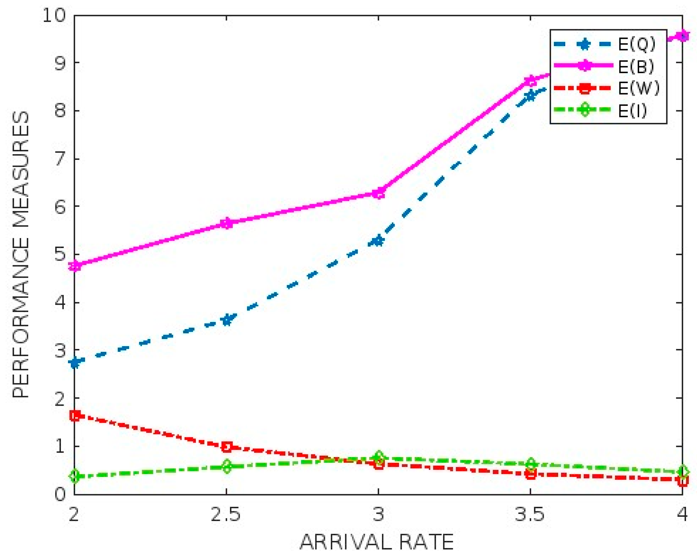
With the assumptions given in Table 2, from Table 3 and Figure 1, it is clear that if the arrival rate increases, the expected number of customers in the queue, expected duration of the busy period of the server, and expected waiting time of a customer in the queue increase whereas the expected duration of the dormant period decreases.

9.1.2. Impact of Breakdown Probability on Performance Metrics

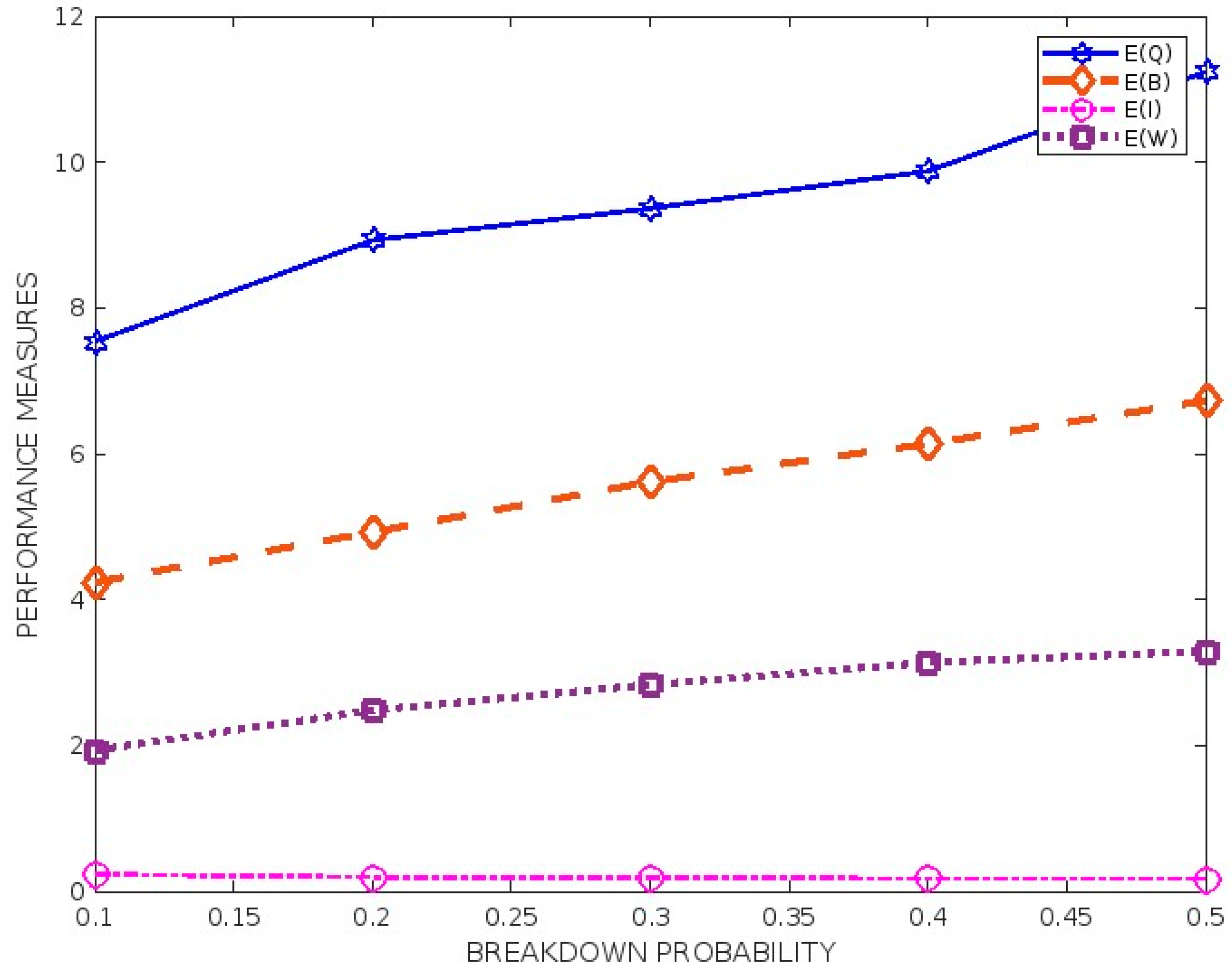
The influence of performance metrics for various failure rates is shown in Table 4 and Figure 2. It can be seen that when the failure rate increases, the predicted inactive period duration and the estimated client waiting time in the queue will also increase.

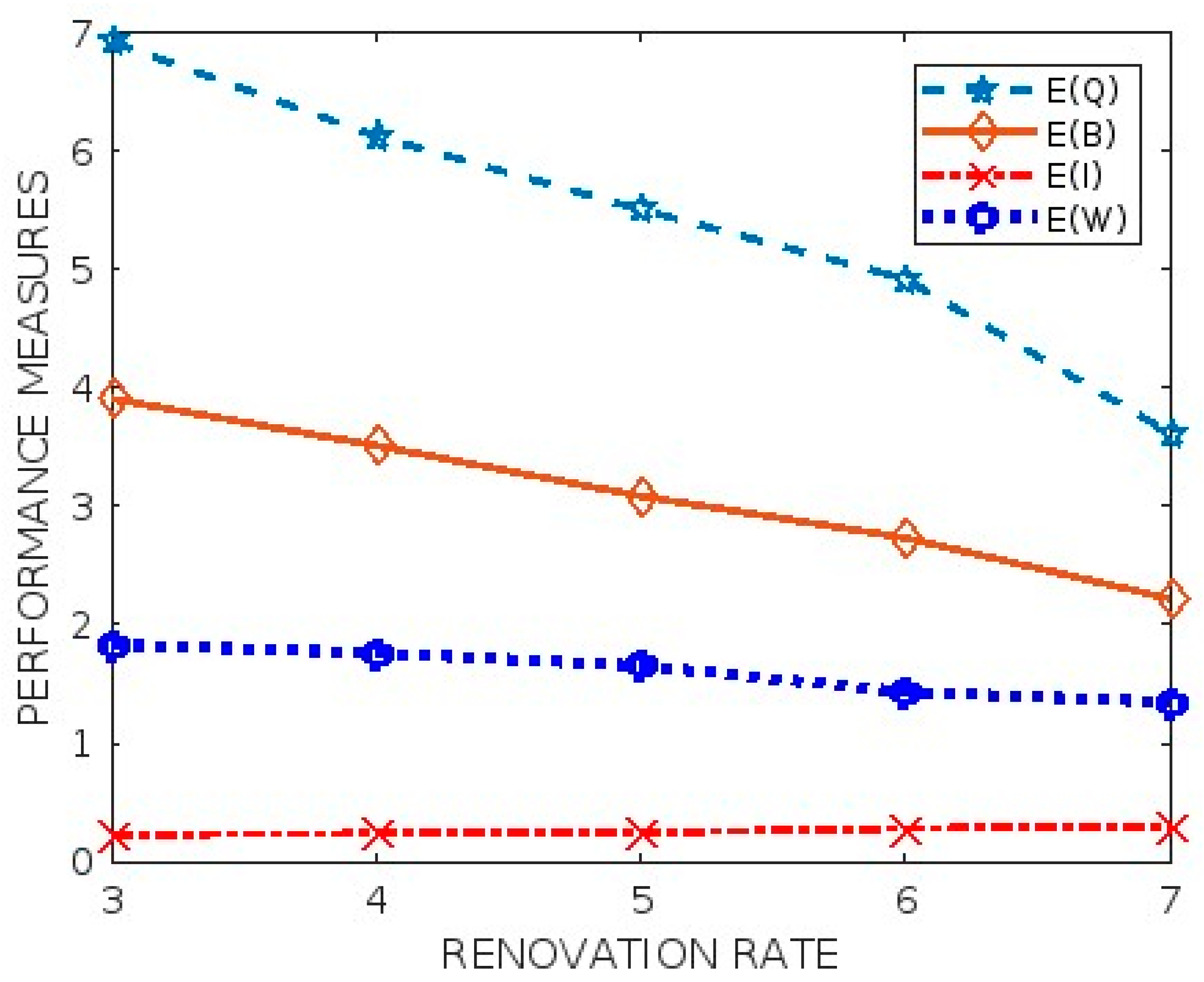
9.1.3. Effects of Renewal Rate on Performance Measures

In Table 5 and Figure 3, the impact on performance metrics for various renewal rates is presented, and it is noted that the expected waiting time in the queue will be decreased whenever the renewal rate increases.

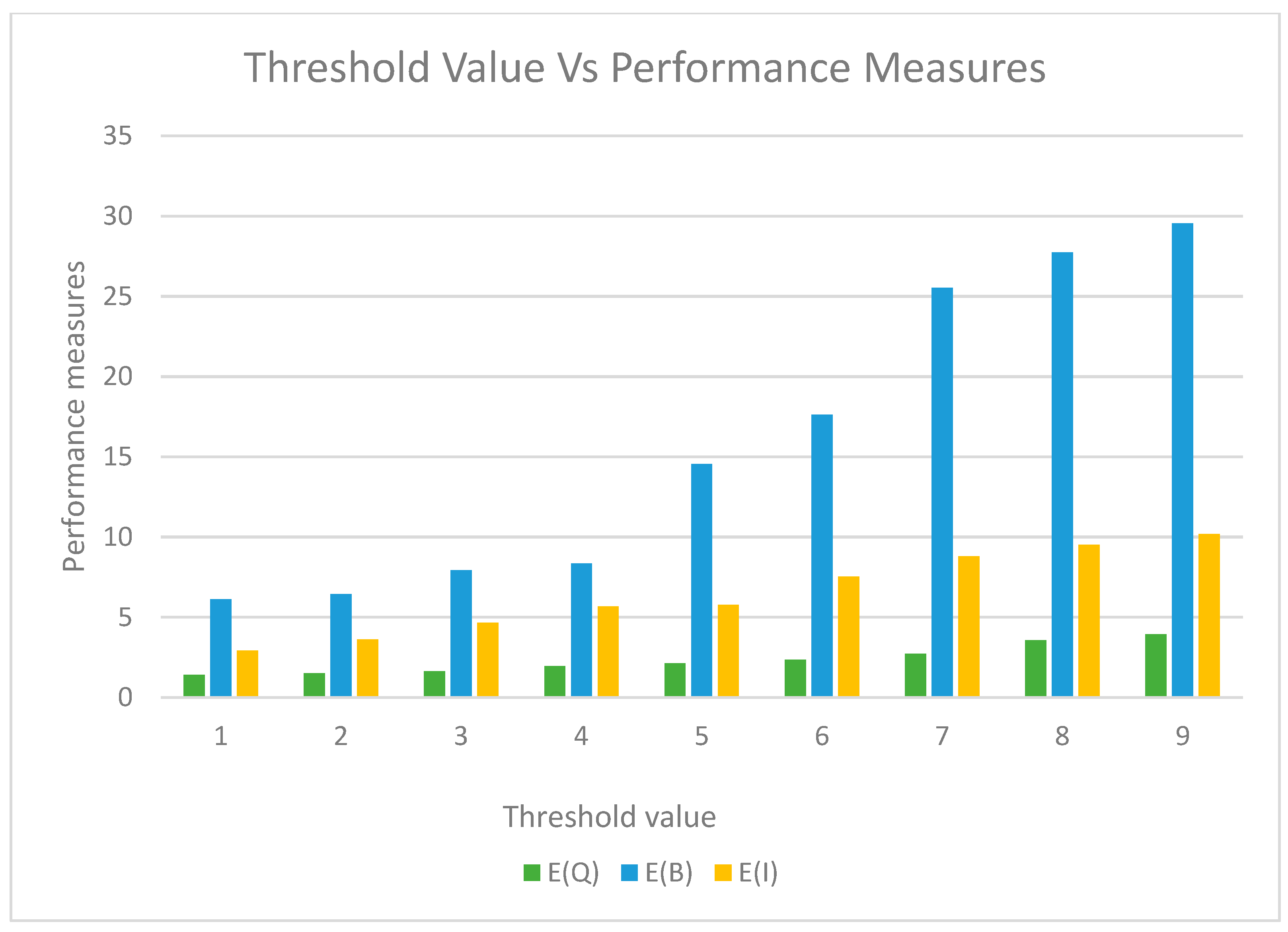
9.1.4. Effects of Threshold Values ‘a’ and ‘N’ on Total Average Cost

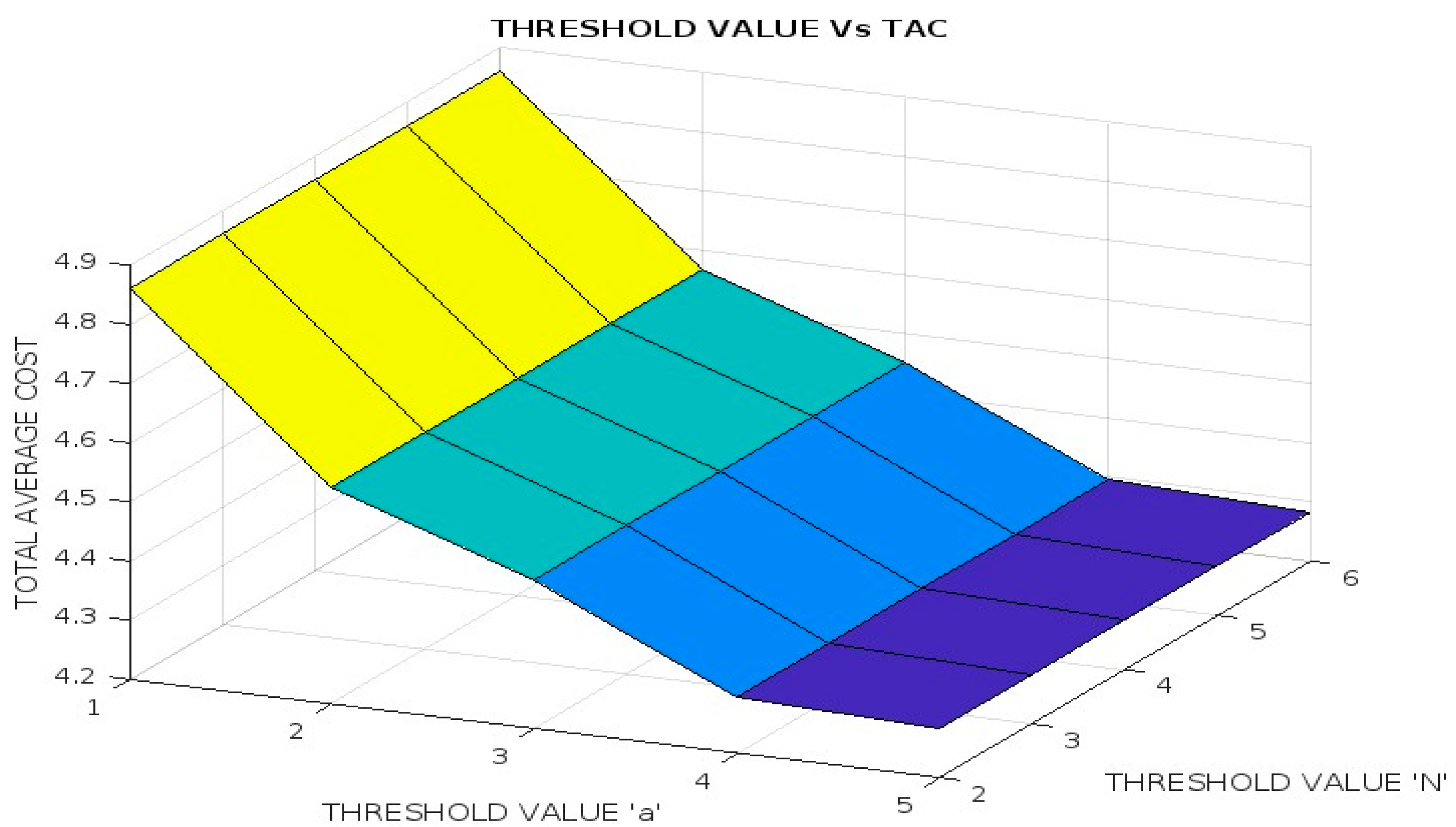
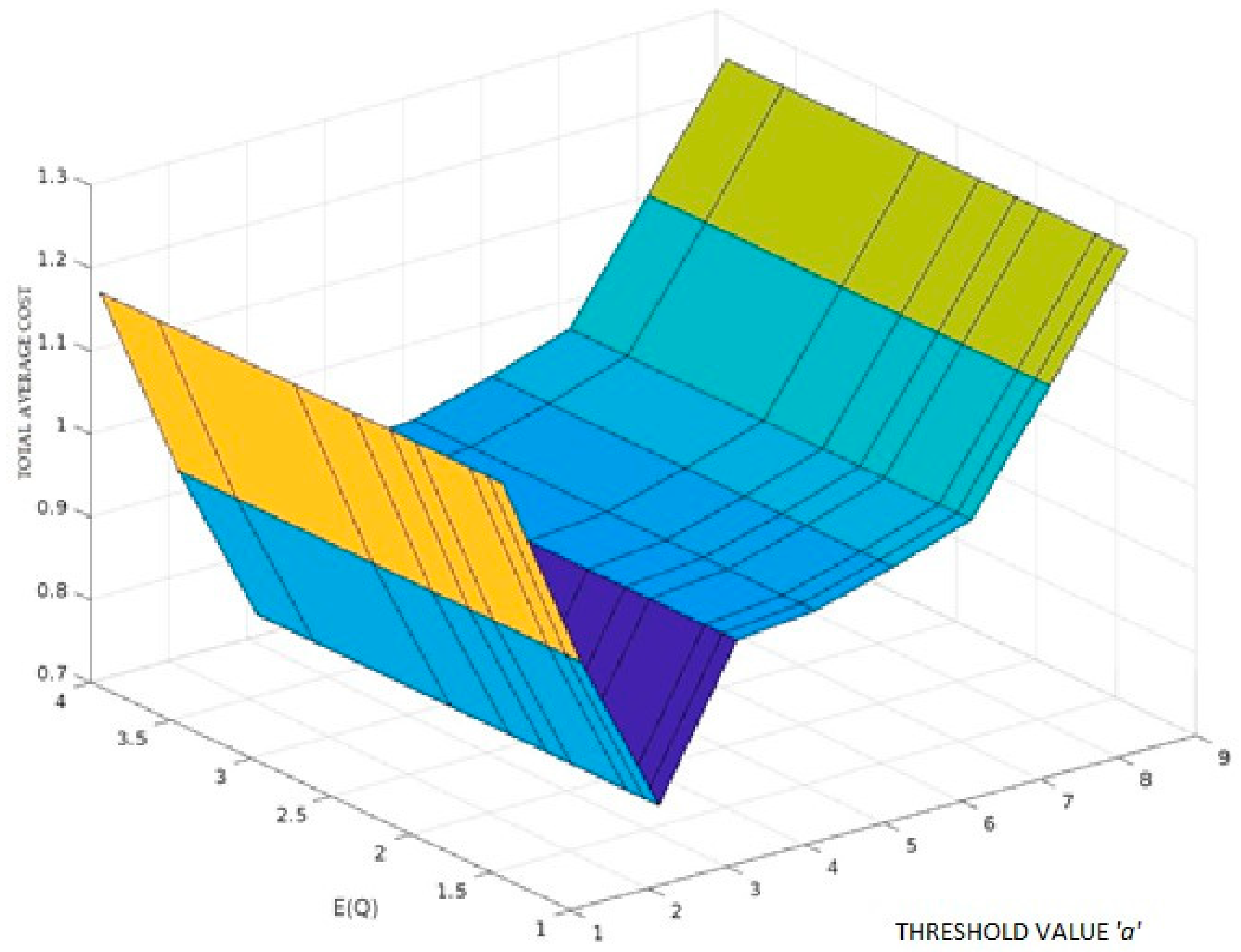
In Table 6 and Figure 4, the effects of the bulk size ‘a’ on the TAC with b = 8 are given. From Table 6 and Figure 5, one can see that, to minimize the overall cost the minimum bulk size ‘a’ should be fixed as 3. Similarly, Table 7 and Figure 5, Figure 6 and Figure 7 suggest to fix the threshold value ‘a’ to minimize the total average cost for various arrival rates, service rates, and vacation rates, and to minimize the overall cost the minimum bulk size should be fixed at a = 5 and N = 6.

9.2. Optimal Cost

Here, we take a look at a numerical example to see how the DRX mechanism might help LTE networks save power. Fixing the values for the thresholds and utilizing the acquired result to minimize the median cost of the entire system is possible. Table 7 shows the impact of different threshold values ‘a’ and ‘N’ on the TAC; setting a = 5 and N = 4.283 yields the lowest total average cost.

10. Conclusions

Here, we have examined two-phase bulk service with active Bernoulli feedback, vacation, and breakdown, as well as bulk arrival in bulk. By utilizing supplementary variable approaches under steady-state settings, we may derive the probability-generating function of the queue size at any given moment. To gauge performance, we estimate things like the number of customers expected to be in line, how long the server’s busy phase will be, how long customers are expected to wait in line, and how long the dormant period will be. We provide concrete numerical examples to ensure that the analytical results are genuine. An application of the proposed queueing model in 4G/5G networks using the DRX mechanism has been given. Additionally, optimum cost analysis has been carried out to minimize the total average cost of the system and make better decisions to fix the threshold value for the service. The uniqueness of the considered model is in the sense that we have introduced an essential two-phase bulk service, renewal time, and two-level control policy for the bulk queueing system. All the introduced parameters are more useful for studying many real-time applications in network systems.

Author Contributions

Conceptualization, S.P.N. and S.D.L.; Data curation, S.P.N. and S.D.L.; Formal analysis, K.K., M.M. and S.D.L.; Investigation, S.P.N. and K.K.; Methodology, S.P.N.; Supervision, S.D.L.; Visualization, M.M. and S.D.L.; Writing—original draft, S.D.L. and S.P.N.; Writing—review and editing, K.K. and M.M. All authors have read and agreed to the published version of the manuscript.

Funding

This work was supported by the project SP2023/074 Application of Machine and Process Control Advanced Methods supported by the Ministry of Education, Youth and Sports, Czech Republic.

Data Availability Statement

The datasets used and/or analyzed during the current study are available from the corresponding author upon reasonable request.

Conflicts of Interest

The authors declare no conflicts of interest.

References

  1. Tian, N.; Zhang, Z.G. Vacation Queueing Models Theory and Applications; International Series in Operations Research & Management Science; Springer: Boston, MA, USA, 2006; Volume 93, ISBN 978-0-387-33721-0. [Google Scholar]
  2. Arumuganathan, R.; Jeyakumar, S. Steady state analysis of a bulk queue with multiple vacations, setup times with N-policy and closedown times. Appl. Math. Model. 2005, 29, 972–986. [Google Scholar] [CrossRef]
  3. Jeyakumar, S.; Senthilnathan, B. Steady state analysis of bulk arrival and bulk service queueing model with multiple working vacations. Int. J. Math. Oper. Res. 2016, 9, 375–394. [Google Scholar] [CrossRef]
  4. Baba, Y. The M/PH/1 queue with working vacations and vacation interruption. J. Syst. Sci. Syst. Eng. 2010, 19, 496–503. [Google Scholar] [CrossRef]
  5. Haridass, M.; Arumuganathan, R. Analysis of a MX/G(a,b)/1 queueing system with vacation interruption. RAIRO-Oper. Res. 2012, 46, 305–334. [Google Scholar] [CrossRef]
  6. Gao, S.; Liu, Z. An M/G/1 queue with single working vacation and vacation interruption under Bernoulli schedule. Appl. Math. Model. 2013, 37, 1564–1579. [Google Scholar] [CrossRef]
  7. Tao, L.; Wang, Z.; Liu, Z. The GI/M/1 queue with Bernoulli-schedule-controlled vacation and vacation interruption. Appl. Math. Model. 2013, 37, 3724–3735. [Google Scholar] [CrossRef]
  8. Pradhan, S.; Gupta, U.C. Modeling and analysis of an infinite-buffer batch-arrival queue with batch-size-dependent service: MX/Gn(a,b)/1. Perform. Eval. 2017, 108, 16–31. [Google Scholar] [CrossRef]
  9. Madan, K.; Abu-Dayyeh, W.; Gharaibeh, M. Steady state analysis of two MX/Ma,b/1 queue models with random breakdowns. Int. J. Inf. Manag. Sci. 2003, 14, 37–51. [Google Scholar]
  10. Jeyakumar, S.; Senthilnathan, B. A study on the behaviour of the server breakdown without interruption in a Mx/G(a,b)/1 queueing system with multiple vacations and closedown time. Appl. Math. Comput. 2012, 219, 2618–2633. [Google Scholar] [CrossRef]
  11. Wu, W.; Tang, Y.; Yu, M. Analysis of an M/G/1 queue with N-policy, single vacation, unreliable service station and replaceable repair facility. Opsearch 2015, 52, 670–691. [Google Scholar] [CrossRef]
  12. Niranjan, S.P.; Chandrasekaran, V.M.; Indhira, K. Stochastic modelling of a two phase bulk service queueing system with active bernoulli feedback, server loss and vacation. Int. J. Pure Appl. Math. 2017, 115, 433–445. [Google Scholar]
  13. Sama, H.; Vemuri, V.; Talagadadeevi, S.; Bhavirisetti, S. Analysis of an N-policy MX/M/1 Two-phase Queueing System with State-dependent Arrival Rates and Unreliable Server. Ingénierie Syst. Inf. 2019, 24, 233–240. [Google Scholar] [CrossRef]
  14. Rao, A.A.; Vedala, N.R.D.; Chandan, K. M/M/1 Queue with N-Policy Two-Phase, Server Start-Up, Time-Out and Breakdowns. Int. J. Recent. Technol. Eng. 2019, 8, 9165–9171. [Google Scholar] [CrossRef]
  15. Enogwe, S.U.; Onyeagu, S.I.; Obiora-Ilouno, H.O. On single server batch arrival queueing system with balking, three types of heterogeneous service and Bernoulli schedule server vacation. Math. Theory Model. 2021, 11, 40. [Google Scholar]
  16. GnanaSekar, M.M.N.; Kandaiyan, I. Analysis of an M/G/1 Retrial Queue with Delayed Repair and Feedback under Working Vacation policy with Impatient Customers. Symmetry 2022, 14, 2024. [Google Scholar] [CrossRef]
  17. Niranjan, S.P. Managerial decision analysis of bulk arrival queuing system with state dependent breakdown and vacation. Int. J. Adv. Oper. Manag. 2020, 12, 351–376. [Google Scholar] [CrossRef]
  18. Blondia, C. A queueing model for a wireless sensor node using energy harvesting. Telecommun. Syst. 2021, 77, 335–349. [Google Scholar] [CrossRef]
  19. Merit, C.K.D.; Haridass, M. A simulation study on the necessity of working breakdown in a state dependent bulk arrival queue with disaster and optional re-service. Int. J. Ad Hoc Ubiquitous Comput. 2022, 41, 1–15. [Google Scholar] [CrossRef]
  20. Deepa, V.; Haridass, M.; Selvamuthu, D.; Kalita, P. Analysis of energy efficiency of small cell base station in 4G/5G networks. Telecommun. Syst. 2023, 82, 381–401. [Google Scholar] [CrossRef]
  21. Niranjan, S.P.; Chandrasekaran, V.M.; Indhira, K. Phase dependent breakdown in bulk arrival queueing system with vacation break-off. Int. J. Data Anal. Tech. Strateg. 2020, 12, 127–154. [Google Scholar] [CrossRef]
  22. Ayyappan, G.; Deepa, T. Analysis of batch arrival bulk service queue with multiple vacation closedown essential and optional repair. Appl. Appl. Math. 2018, 13, 2. [Google Scholar]
  23. Niranjan, S.P.; Komala Durga, B.; Thangaraj, M. Steady-State Analysis of Bulk Queuing System with Renovation, Prolonged Vacation and Tune-Up/Shutdown Times. In Proceedings of the 2nd International Conference on Mathematical Modeling and Computational Science, Surat, India, 5–6 February 2022; Peng, S.-L., Lin, C.-K., Pal, S., Eds.; Springer Nature: Singapore, 2022; pp. 35–48. [Google Scholar]
  24. Nithya, R.P.; Haridass, M. Cost optimisation and maximum entropy analysis of a bulk queueing system with breakdown, controlled arrival and multiple vacations. Int. J. Oper. Res. 2020, 39, 279–305. [Google Scholar] [CrossRef]
  25. Enogwe, S.; Obiora-Ilouno, O.; Enogwe, S.; Obiora-Ilouno, H. Effects of Re-neging, Server Breakdowns and Vacation on a Batch Arrival Single Server Queueing System with Three Fluctuating Modes of Service. Open J. Optim. 2020, 9, 105–128. [Google Scholar] [CrossRef]
  26. Khan, I.; Paramasivam, R. Reduction in Waiting Time in an M/M/1/N Encouraged Arrival Queue with Feedback, Balking and Maintaining of Reneged Customers. Symmetry 2022, 14, 1743. [Google Scholar] [CrossRef]
  27. Ammar, S.; Rajadurai, P. Performance Analysis of Preemptive Priority Retrial Queueing System with Disaster under Working Breakdown Services. Symmetry 2019, 11, 419. [Google Scholar] [CrossRef]
  28. Hanukov, G.; Shoval, S. A Model for a Vacation Queuing Policy Considering Server’s Deterioration and Recovery. Mathematics 2023, 11, 2640. [Google Scholar] [CrossRef]
  29. Xing, R.; Cai, X.; Liu, Y.; Yang, Z.; Wang, Y.; Peng, B. Study on Queue Length in the Whole Process of a Traffic Accident in an Extra-Long Tunnel. Mathematics 2023, 11, 1773. [Google Scholar] [CrossRef]
  30. Chaudhry, M.; Datta Banik, A.; Barik, S.; Goswami, V. A Novel Computational Procedure for the Waiting-Time Distribution (In the Queue) for Bulk-Service Finite-Buffer Queues with Poisson Input. Mathematics 2023, 11, 1142. [Google Scholar] [CrossRef]
  31. Rece, L.; Vlase, S.; Ciuiu, D.; Neculoiu, G.; Mocanu, S.; Modrea, A. Queueing Theory-Based Mathematical Models Applied to Enterprise Organization and Industrial Production Optimization. Mathematics 2022, 10, 2520. [Google Scholar] [CrossRef]
  32. Demircioglu, M.; Bruneel, H.; Wittevrongel, S. Analysis of a Discrete-Time Queueing Model with Disasters. Mathematics 2021, 9, 3283. [Google Scholar] [CrossRef]
  33. Marcel, F. Neuts A General Class of Bulk Queues with Poisson Input. Ann. Math. Stat. 1967, 38, 759–770. [Google Scholar] [CrossRef]
  34. Cox, D.R. The analysis of non-Markovian stochastic processes by the inclusion of supplementary variables. Math. Proc. Camb. Philos. Soc. 1955, 51, 433–441. [Google Scholar] [CrossRef]
Figure 1. Arrival rate versus performance metrics.
Mathematics 12 00075 g001
Figure 2. Breakdown probability vs. performance metrics.
Mathematics 12 00075 g002
Figure 3. Renewal rate vs. performance metrics.
Mathematics 12 00075 g003
Figure 4. Threshold value ‘a’ vs. Performance metrics.
Mathematics 12 00075 g004
Figure 5. Threshold value ‘a’ vs. TAC.
Mathematics 12 00075 g005
Figure 6. Threshold values ‘a’ and ‘N’ versus TAC.
Mathematics 12 00075 g006
Figure 7. Threshold value vs. TAC for λ = 2 ,   b = 8 ,   µ 1 = µ 2 = 2.0 ,   = 1 ,   γ = 3 ,   η = 4 ,   α = 6 .
Mathematics 12 00075 g007
Table 1. Notations.
Table 1. Notations.
Cumulative Distribution FunctionProbability Distribution FunctionLaplace–Stieltjes TransformRemaining Service Time
First essential service S ( y ) s ( y ) S ~ ( θ ) S 0 ( y )
Second essential service S 2 ( y ) s 2 ( y ) S ~ 2 ( θ ) S 2 0 ( y )
VacationV( y ) v ( y ) V ~ ( θ ) V 0 ( y )
Renewal timeR( y ) r ( y ) R ~ ( θ ) R 0 ( y )
Preparatory workA ( y ) a ( y ) A ~ ( θ ) A 0 ( y )
Table 2. Parameters and Notations.
ParameterDistributionNotations
Arrival ratePoisson distribution λ 1
First essential service2-Erlang distribution µ 1
Second essential service2-Erlang distribution µ 2
VacationExponential distribution
RenewalExponential distributionη
Setup timeExponential distribution α
Table 3. Arrival rate versus performance metrics.
λ 1 E(Q)E(B)E(I)E(W)
3.03.75415.21232.54541.2212
3.44.54326.52162.11812.3321
4.05.66327.99341.54324.1254
4.57.11239.12111.12145.4313
5.08.824611.23210.54326.2242
5.69.654212.45320.32437.3232
6.010.434214.23210.12119.1214
E(Q)—Expected number of customers in the queue; E(B)—Expected duration of the busy period of the server; E(W)—Expected waiting time of a customer in the queue; E(I)—Expected duration of the dormant period. (For minimum server capacity a = 2, maximum server capacity b = 4, vacation rate = 10, renewal rate η = 8, breakdown probability δ   = 0.2, feedback probability β = 0.5 ).
Table 4. Breakdown of probability versus performance measures.
δ E(Q)E(B)E(I)E(W)
0.510.23438.54728.22319.1227
0.611.45329.23457.853511.2236
0.713.123111.45325.123213.5645
0.815.294112.63413.221215.6543
0.916.398713.98712.154516.6432
E(Q)—Expected number of customers in the queue; E(B)—Expected duration of the busy period of the server; E(W)—Expected waiting time of a customer in the queue; E(I)—Expected duration of the dormant period.
Table 5. Renewal ratio versus performance measures.
Renewal RateE(Q)E(B)E(I)E(W)
26.9326.65324.15345.2345
46.1346.25435.67343.4564
65.5135.23217.47651.5643
84.9274.14318.24511.1457
103.6232.925610.15430.4381
E(Q)—Expected number of customers in the queue; E(B)—Expected duration of the busy period of the server; E(W)—Expected waiting time of a customer in the queue; E(I)—Expected duration of the dormant period.
Table 6. Threshold Value ‘a’ vs. Total Average Cost.
aE(Q)E(B)E(I)TAC
21.35636.28742.89631.2753
31.43896.64213.75240.8754
41.51297.79434.73270.6798
51.83198.48625.56390.9875
62.034513.57825.80320.9234
72.242718.45927.67310.9875
82.819324.57288.69320.9109
93.673826.84329.45891.5098
103.892130.173210.58211.4326
E(Q)—Expected number of customers in the queue; E(B)—Expected duration of the busy period of the server; E(I)—Expected duration of the dormant period. Arrival rate   λ 1 = 2 ; m a x i m u m   s e r v e r   c a p a c i t y   b = 8 ,   s e r v i c e   r a t e   o f   F E S   µ 1 = s e r v i c e   r a t e   o f   S E S   µ 2 = 2.0 , v a c a t i o n   r a t e   = 1 , b r e a k   d o w n   p r o b a b i l i t y   δ   =   3 , r e n e w a l   r a t e   η = 4 , s e t   u p   t i m e   α = 6 .
Table 7. Threshold value versus TAC.
Threshold Value ′N′ to Start Bulk Service
Threshold value ′a
to start service
N2345678910
a TAC
14.8614.7324.7464.9655.5835.9516.2476.3657.483
2 4.5674.5184.8725.4325.6736.0846.2476.941
3 4.4524.6724.7924.8645.2725.4315.934
4 4.2954.6434.8215.0935.1875.531
5 4.2834.3144.4215.0425.467
6 4.3154.4104.9895.035
7 4.3574.7455.021
8 4.5784.995
9 4.982
Minimum TAC occurs when a = 5 and N = 6.
Disclaimer/Publisher’s Note: The statements, opinions and data contained in all publications are solely those of the individual author(s) and contributor(s) and not of MDPI and/or the editor(s). MDPI and/or the editor(s) disclaim responsibility for any injury to people or property resulting from any ideas, methods, instructions or products referred to in the content.