Handling Non-Linearities in Modelling the Optimal Design and Operation of a Multi-Energy System

Abstract

Multi-energy systems (MESs) combining different energy carriers like electricity and heat allow for more efficient and sustainable energy solutions. However, optimizing the design and operation of MESs is challenging due to non-linearities in the mathematical models used, especially the performance curves of technologies like combined heat and power units. Unlike similar work from the literature, this paper proposes an improved piecewise linearization method to efficiently handle the non-linearities, models an MES as a multi-objective mixed-integer linear program (MILP), and solves the optimization problem over a year with hourly resolution to enable detailed operation and faithful system design. The method uses fewer linear pieces to approximate non-linear functions compared to a standard technique, resulting in lower complexity while preserving accuracy. The MES design and operation problem maximizes cost reduction and the rate of renewable energy sources. A case study on an MES with electricity and heat over one year with hourly resolution demonstrates the effectiveness of the new method. It allows for solving a long-term MES optimization problem in reasonable computation times.

1. Introduction

Domestic consumers and industrial facilities require different kinds of energy, such as heat, electricity, and natural gas. Different energy carriers have traditionally been used and planned separately, but their combination can have an added value in terms of energy efficiency, reliability, cost, and environmental impact [1,2]. Recently, multi-energy systems (MES), e.g., combining heat, electricity and gas, have attracted increasing attention in energy engineering as they are seen as good candidates to drastically reduce CO₂ emissions [1,3]. Accordingly, the optimization of such systems has become a crucial research topic and should help answer questions related to the efficient integration of renewable energy sources (RES) or increased uses of energy storage solutions.

The optimization of an MES mainly relates to the optimization of the design and the optimization of the operation of the system, which can be optimized independently or jointly [4,5]. The latter aims at planning the use of the different production units, energy storage systems, etc., installed in the MES, to meet the energy demand at each time step for each energy carrier of the MES. Given a set of production or storage units, the optimization process determines which and when the units have to be switched on/off, generally in order to minimize an objective function related to cost or emissions [6].

Optimizing the design of MESs independently of the operation consists of selecting which production technologies to use in the system, their configuration in the energy networks, their optimal installed capacities, etc. The design can be optimized using fixed rules for the operation, such as a predefined merit order, as in [7]. However, works related to the design optimization very often also study operation optimization. These studies are interested in optimizing the design and the operation jointly as a single problem to find the optimal configuration of the MES.

In the works that optimize the MES as a whole, [8,9,10] propose a mono-objective approach that seeks to minimize the total cost of an MES, represented as an energy hub. Other works address the problem through a multi-objective perspective, where they try to minimize the costs of the system and maximize its environmental performance [7,11,12,13,14]. These objective functions can be expressed in different ways. For example, the optimization of the environmental impact can be translated into a maximization of the rate of renewable energy [7] or a minimization of the CO₂ emission rate [11,12,14,15], or a minimization of the environmental cost [13]. The optimization of the costs can be calculated as the minimization of total costs [14,16], the minimization of the cost of power generation [13], the maximization of profits [17,18], or the minimization of costs compared to a reference system [7,19].

Two crucial points of these works are the time horizon and the temporal resolution taken into account for optimizing the system. The temporal resolution has a big impact on the accuracy of the model when there is a large share of renewable energy sources in the system [16,20]. Most works generally optimize energy systems over short representative time periods, for example a few days or a few weeks. Ref. [12] uses six representative periods representing the average consumption during the day and during the night in winter, summer, and at mid-season for an MES with electricity, heating, hot water, and cooling. Ref. [15] uses twelve representative periods to represent the average consumption over each month of the year for an MES with electricity and heat. Ref. [21] optimizes a model with a shiftable load over a period of three years using sequential 24 h time horizons for an MES with electricity, heat, and cooling. Ref. [22] optimize three representative days per month with an hourly resolution for the twelve months of the year for an MES with electricity and heat. Ref. [11] presents several methods using coupled design days to allow for optimizing most of the system using representative design days while preserving a continuity in the energy storage using a full-year optimization for an MES with electricity and heat. Ref. [14] studies the effect of different scenarios for combined cooling, heating, and power (CCHP) units using three representative days. However, there are always errors due to the aggregation of time-series into representative days [23]. In a general way, representative design day methods are less efficient when integrating energy storage in the system due to the dynamic aspect of the storage.

Depending on the complexity of the proposed models, the authors use either exact methods or metaheuristics to solve the optimization problem. The former methods solve the model to optimality, but are not able to solve large-sized problems. The latter do not guarantee the optimality but render good (i.e., near-optimal) solutions with a small gap in a reasonable computation time [24]. Metaheuristics are also practical when solving non-linear optimization models; however, they become less efficient when dealing with optimization problems with a huge number of integer decision variables [25]. Ref. [26] optimizes an MES and its thermal network by decomposing the problem in two subproblems: a mixed-integer linear programming formulation optimizes the MES without considering the thermal network, and a quadratically constrained programming formulation optimizes the thermal network. Ref. [10] use a Particle Swarm Optimization metaheuristic to optimize an MES with heat and power storage, and [13] uses a Bee Colony metaheuristic to optimize an MES with a CCHP unit over a single day. To cope with this issue and as a combination of both exact and metaheuristics, matheuristics step in to benefit from the advantages of both methods. For instance, the heuristic component (i.e., could be a metaheuristic) of the method is used to handle/determine binary decision variables, while the exact component determines the remaining continuous/integer decision variables [27]. The two components cooperate in an iterative manner to solve the problem, as in [12,15] for MES. However, they do not guarantee optimality, and can still be hard to solve for longer time horizons. Next to that, non-linearities are sometimes solved using linearization techniques. For example, the work of [22] linearizes the non-linear part-load efficiency of combined heat and power (CHP) units using binary variables in a mixed integer linear programming model. Ref. [26] uses 1D and 2D piecewise linearization methods, including the triangle method proposed by [28], to linearize the performance curves of technologies in an MES. Moreover, various approximation methods of different complexities can be used to approximate these types of part-load efficiencies [29]. Ref. [30] considers linear efficiencies with different efficiency functions for different installed capacities. However, a linear efficiency function can greatly overestimate or underestimate the real value. Once again, these types of problem are hard to solve for large-size instances (e.g., long time horizons) because of the introduction of integer decision variables.

To leverage the complexity of the optimization of MESs, different simplifications are employed. The most straightforward simplification is the optimization of the system over a short time horizon, e.g., 24 h instead of a full year [22]. This does not allow for a long-term optimization, as the energy demands can vary significantly over the year, and it makes it harder to integrate energy storage into the model. Some other studies use a large time step; for instance, some consider an average value of energy demand over a certain period of time that can range from half a day to a full month [31]. Using the latter simplification, the optimization of the operation is less accurate since the variations in day-to-day demand are canceled out by the averaged values. The use of design days—which are typical days representative of a period of time—improves the accuracy of the optimization, but they can also cancel out the extreme values, which must be taken into account to ensure a good design of the MES when the time-series data intervene in the constraints [23]. Another simplification is the decomposition of the main problem into sub-problems; for example, optimizing a long period of time day by day.

In this paper, we address the three above-identified problems. First, we model an MES in terms of a multi-objective non-linear programming model to optimize simultaneously the design and the optimization of the MES. Second, we present different methods of linearizing the non-linear parts of this mathematical model, and we propose an improved linearization method, which generates less complex models than the classical one from the literature. Third, we solve the problem with a time resolution of one hour, sufficient to optimize the operation, and over a long period of time (one year) to allow faithful optimization of the design. Finally, we do a comparative analysis to evaluate the performance of the proposed method.

The aim of the research presented here is to optimize a multi-energy system over a full year, with a time resolution of one hour. To achieve this, it is necessary to take into account the non-linearities of the model, and we therefore propose a linearization method that can approximate a non-linear function efficiently, i.e., with a better approximation of the function and with a faster computation time than a standard method from the literature.

The remainder of this paper is organized as follows. In Section 2, we define the problem we are dealing with and formulate it as a mathematical program. This model contains non-linear elements, which is why in Section 3 we detail three different resolution techniques, among which is an original proposal. To validate the proposed model and the resolution techniques, we apply in Section 4 the model on a real-world problem. We study the solutions obtained through the three resolution methods in Section 5.1 and discuss the results in Section 5.2, before drawing some conclusions in Section 6.

2. Problem Definition and Formulation

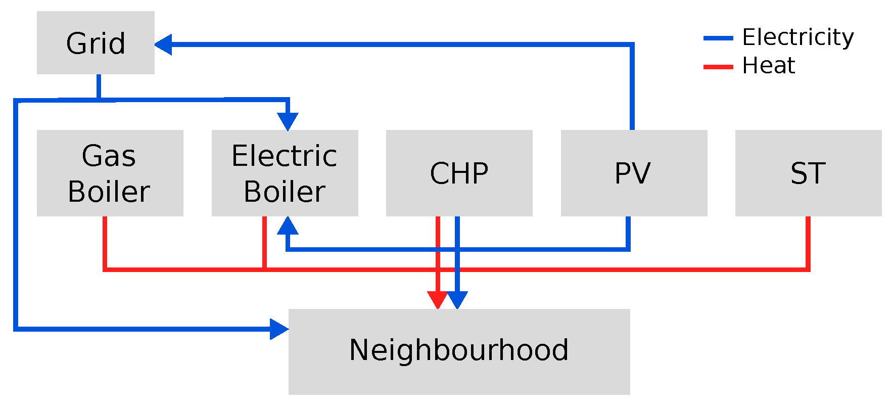
In this article, we study the MES system illustrated in Figure 1 involving three energy carriers: electricity, heat, and gas (the latter being only used as fuel). The main goal is to meet the energy demand of the system, which is a demand for heat and electricity over a time horizon of one year with a resolution of one hour. For this purpose, different technologies are used:

• a combined heat and power unit (CHP) which provides heat and electricity from gas;
• an electric boiler (EB) which provides heat;
• a gas boiler (GB), which also provides heat;
• photovoltaic (PV) panels which generate electricity;
• solar thermal (ST) panels which generate heat.

The latter two technologies are considered as RES. Electricity can also be bought from the grid, and the surplus electricity produced by the PV panels can be sold to the grid. We also consider here that each technology must be installed with a minimal capacity, even if they are not used throughout the year.

The energy demand must be met by the system while optimizing two objectives: minimizing the cost of the system and maximizing the rate of renewable energy sources.

We formulate the above problem as a mathematical program model.

Table 1. Notation.

Notation	Description
$\mathcal{N}=\{e,h,g\}$	Set of energy carriers, e (electricity), h (heat), g (gas, only used as fuel)
$\mathcal{M}=\{CHP,GB,EB,PV,ST\}$	Set of technologies
$\mathcal{T}=\{1,2,\dots ,8760\}$	Set of hours of the year
$P_{i,j,t}$	Energy of type $i\in \mathcal{N}$ generated by technology $j\in \mathcal{M}$ at time $t\in \mathcal{T}$
$F_{i,j,t}$	Energy of type $i\in \mathcal{N}$ absorbed by technology $j\in \mathcal{M}$ (as fuel) at time $t\in \mathcal{T}$
$U_{i,t}$	Energy of type $i\in \mathcal{N}$ imported at time $t\in \mathcal{T}$
$V_{i,t}$	Energy of type $i\in \mathcal{N}$ exported at time $t\in \mathcal{T}$
$L_{i,t}$	Demand of energy of type $i\in \mathcal{N}$ at time $t\in \mathcal{T}$

summarizes the notation used in this work.

The mathematical formulation of the optimization problem and its resolution lead to the determination of optimal values for a certain number of decision variables. These decision variables are of two types here, namely design and operation variables. The design variables (

Table 2. Design decision variables.

Variable	Description
${\mathit{P}}_{\mathit{CHP},\mathit{nom}}$	Electrical rated power of the CHP ($\mathrm{k}{\mathrm{W}}_{\mathrm{e}}$, [$P_{CHP,nom}^{min},P_{CHP,nom}^{max}$])
${\mathit{P}}_{\mathit{GB},\mathit{nom}}$	Thermal rated power of the GB ($\mathrm{k}{\mathrm{W}}_{\mathrm{th}}$, [$P_{GB,nom}^{min},P_{GB,nom}^{max}$])
$\begin{array}{c}\hfill {\mathit{P}}_{\mathit{EB},\mathit{nom}}\end{array}$	Thermal rated power of the EB ($\mathrm{k}{\mathrm{W}}_{\mathrm{th}}$, [$P_{EB,nom}^{min},P_{EB,nom}^{max}$])
$\begin{array}{c}\hfill {\mathit{A}}_{\mathit{PV}}\end{array}$	Area of PV (${\mathrm{m}}^2$, [$A_{PV}^{min},A_{PV}^{max}$])
$\begin{array}{c}\hfill {\mathit{A}}_{\mathit{ST}}\end{array}$	Area of ST (${\mathrm{m}}^2$, [$A_{ST}^{min},A_{ST}^{max}$])

) are used to determine the size of the units (the rated power of the generators or the area of solar panels), and a minimum value for each of these variables ensures that the related technologies are used, as the goal here is not to decide which technology is present in the system. The operation variables (

Table 3. Operation decision variables at time $t\in \mathcal{T}$.

Variable	Description
$\begin{array}{c}\hfill {\mathit{P}}_{\mathit{e},\mathit{CHP},\mathit{t}}\end{array}$	Electricity generated by the CHP, $\forall t\in \mathcal{T}$
$\begin{array}{c}\hfill {\mathit{P}}_{\mathit{h},\mathit{CHP},\mathit{t}}\end{array}$	Heat generated and used by CHP (extra heat is lost), $\forall t\in \mathcal{T}$
$\begin{array}{c}\hfill {\mathit{F}}_{\mathit{g},\mathit{CHP},\mathit{t}}\end{array}$	Gas used as fuel by the CHP, $\forall t\in \mathcal{T}$
$\begin{array}{c}\hfill {\mathit{P}}_{\mathit{h},\mathit{GB},\mathit{t}}\end{array}$	Heat generated by the GB, $\forall t\in \mathcal{T}$
$\begin{array}{c}\hfill {\mathit{P}}_{\mathit{h},\mathit{EB},\mathit{t}}\end{array}$	Heat generated by EB
$\begin{array}{c}\hfill {\mathit{P}}_{\mathit{e},\mathit{PV},\mathit{t}}\end{array}$	Power usage of PV at time t (extra power is sold to the grid)
$\begin{array}{c}\hfill {\mathit{P}}_{\mathit{h},\mathit{ST},\mathit{t}}\end{array}$	Power usage of ST at time t (extra heat is lost)
$\begin{array}{c}\hfill {\mathit{U}}_{\mathit{e},\mathit{t}}\end{array}$	Electricity bought from the grid at time t
$\begin{array}{c}\hfill {\mathit{V}}_{\mathit{e},\mathit{t}}\end{array}$	Electricity sold to the grid at time t

) are used to optimize the operation of the system at each time step $t\in \mathcal{T}$, deciding how much energy is produced by each unit and how much is bought or sold. In this work, the decision variables of the mathematical model are highlighted in bold and blue (e.g., $\begin{array}{c}\hfill {\mathit{P}}_{\mathit{CHP},\mathit{nom}}\end{array}$ in Table 2), and mathematical terms depending on these variables are in bold, e.g., ${\mathit{F}}_{\mathit{g},\mathit{GB},\mathit{t}}$.

The system is also characterized by a certain number of parameters that define its intrinsic functioning (i.e., efficiency coefficients, costs, etc.). These parameters are presented in

Table 4. Parameters.

Parameter	Description
$P_{CHP,nom}^{min}$, $P_{CHP,nom}^{max}$	Minimum and maximum nominal power of the CHP
$P_{GB,nom}^{min}$, $P_{GB,nom}^{max}$	Minimum and maximum nominal power of the GB
$P_{EB,nom}^{min}$, $P_{EB,nom}^{max}$	Minimum and maximum nominal power of the EB
$A_{PV}^{min}$, $A_{PV}^{max}$	Minimum and maximum area of the PV panels
$A_{ST}^{min}$, $A_{ST}^{max}$	Minimum and maximum area of the ST panels
$L_{e,t}$	Electricity demand of the system at time $t\in \mathcal{T}$
$L_{h,t}$	Heat demand of the system at time $t\in \mathcal{T}$
a, b, c	Electrical efficiency coefficients of the CHP
${\eta }_{th,CHP}$	Thermal efficiency of the heat recuperation system of the CHP
${\eta }_{GB}$	Efficiency of the GB
${\eta }_{EB}$	Efficiency of the EB
${\eta }_{DC/AC}$	PV inverters’ efficiency
${\eta }_{ref}$	Reference efficiency for PV
$G_{\beta ,t}$	Global solar radiation at time $t\in \mathcal{T}$
$\alpha$	Temperature coefficient of PV
$T_{ref}$	Reference temperature
$T_{a,t}$	Outdoor temperature at time $t\in \mathcal{T}$
$P_{panel,nom}$	Nominal power of a PV panel
$A_{panel}$	Area of a PV panel
${\eta }_0$	Optical efficiency of ST
$U_{loss}$	Thermal loss coefficient of ST
$T_{w,m}$	Mean water temperature in the ST collector
$A_{total}$	Total area available for solar panels
${\gamma }_{inv,j}$	Investment cost for technology $j\in \mathcal{M}$
${\gamma }_{O\&M,j,f}$	Fixed part of the operation cost for technology $j\in \mathcal{M}$
${\gamma }_{O\&M,j,v}$	Variable part of the operation cost for technology $j\in \mathcal{M}$
$C_{gr,t}$	Cost of electricity bought from the grid at time $t\in \mathcal{T}$
$C_g$	Cost of gas bought
$I_{gr}$	Price of electricity sold to the grid

.

Determining the cost of the system requires the calculation of various investment and operation costs for each of the technologies.

Table 5. Investment and operation costs of the technologies.

Technology j	${\mathit{C}}_{\mathit{inv},\mathit{j}}$	${\mathit{C}}_{\mathit{O}\&\mathit{M},\mathit{j}}$
$\mathit{CHP}$	${\gamma }_{inv,CHP}\begin{array}{c}\hfill {\mathit{P}}_{\mathit{CHP},\mathit{nom}}\end{array}$	${\gamma }_{O\&M,CHP,v}{\sum }_{t\in \mathcal{T}}\begin{array}{c}\hfill {\mathit{P}}_{\mathit{e},\mathit{CHP},\mathit{t}}\end{array}$
$\mathit{GB}$	${\gamma }_{inv,GB}\begin{array}{c}\hfill {\mathit{P}}_{\mathit{GB},\mathit{nom}}\end{array}$	${\gamma }_{O\&M,GB,f}\begin{array}{c}\hfill {\mathit{P}}_{\mathit{GB},\mathit{nom}}\end{array}$
$\mathit{EB}$	${\gamma }_{inv,EB}\begin{array}{c}\hfill {\mathit{P}}_{\mathit{EB},\mathit{nom}}\end{array}$	${\gamma }_{O\&M,EB,f}\begin{array}{c}\hfill {\mathit{P}}_{\mathit{EB},\mathit{nom}}\end{array}+{\gamma }_{O\&M,EB,v}{\sum }_{t\in \mathcal{T}}\begin{array}{c}\hfill {\mathit{P}}_{\mathit{h},\mathit{EB},\mathit{t}}\end{array}$
$\mathit{PV}$	${\gamma }_{inv,PV}{P}_{panel,nom}\begin{array}{c}\hfill {\mathit{A}}_{\mathit{PV}}\end{array}/A_{panel}$	${\gamma }_{O\&M,PV,f}{P}_{panel,nom}\begin{array}{c}\hfill {\mathit{A}}_{\mathit{PV}}\end{array}/A_{panel}$
$\mathit{ST}$	${\gamma }_{inv,ST}\begin{array}{c}\hfill {\mathit{A}}_{\mathit{ST}}\end{array}$	${\gamma }_{O\&M,ST,f}\begin{array}{c}\hfill {\mathit{A}}_{\mathit{ST}}\end{array}$

details the calculation of the investment costs $C_{inv,j}$ and the operation and maintenance costs $C_{O\&M,j}$ of different technologies $j\in \mathcal{M}$. The investment costs are proportional to the installed capacities, i.e., the power rate of the production units and the area of RES. The operation and maintenance costs depend on a fixed part proportional to the installed capacity, and a variable part proportional to the output power.

We recall that one of the objectives of this work is to minimize the total cost of the system. This goal can be translated as the maximization of a cost reduction with respect to a reference system. We therefore consider a particular reference state of the system, in which only the GB is used to generate the heat and where electricity is bought from the grid.

The annual cost of the reference system, $AT{C}_{ref}$, is computed as:

$$AT{C}_{ref}=C_{O\&M,GB}^{ref}+\mathit{crf}\ast C_{inv,GB}^{ref}+{\sum }_{t\in \mathcal{T}}(C_{gr,t}{U}_{e,t}^{ref}+C_g{F}_{g,GB,t}^{ref}).$$

(1)

Moreover, the annual cost of the MES, $AT{C}_{MES}$, is given by:

$$\begin{array}{c}AT{C}_{MES}={\sum }_{j\in \mathcal{M}}({\mathit{C}}_{\mathit{O}\&\mathit{M},\mathit{j}}+\mathit{crf}\ast {\mathit{C}}_{\mathit{inv},\mathit{j}})-{\sum }_{t\in \mathcal{T}}{I}_{gr}\begin{array}{c}\hfill {\mathit{V}}_{\mathit{e},\mathit{t}}\end{array}\hfill \\ \hspace{1em}\hspace{1em}\hspace{1em}\hspace{1em}\hspace{1em} +{\sum }_{t\in \mathcal{T}}(C_{gr,t}{\mathit{U}}_{\mathit{e},\mathit{t}}+C_g({\mathit{F}}_{\mathit{g},\mathit{CHP},\mathit{t}}+{\mathit{F}}_{\mathit{g},\mathit{GB},\mathit{t}}))\hfill \end{array}$$

(2)

$\mathit{crf}$ in those two equations is the capital recovery factor and represents the present value of an annuity based on a number of annuities n and a discount factor i. It is expressed as $\mathit{crf}=i{(1+i)}^n/({(1+i)}^n-1)$.

Consequently, the annual cost reduction of the MES compared to the reference system can be calculated as:

$$ATCR=100\ast (1-\frac{{\mathit{ATC}}_{\mathit{MES}}}{AT{C}_{ref}})$$

(3)

The second objective stated above concerns the RES rate, which is to be maximized. The percentage of the energy demand covered by RES, namely $PV$ panels for the electricity demand and $ST$ for the heat demand, is calculated as follows:

$${\tau }_{RES}=100\ast \frac{{\sum }_{t\in \mathcal{T}}({\mathit{P}}_{\mathit{e},\mathit{PV},\mathit{t}}+{\mathit{P}}_{\mathit{h},\mathit{ST},\mathit{t}})}{{\sum }_{t\in \mathcal{T}}(L_{e,t}+L_{h,t})}$$

(4)

The various components and the decision variables of the MES under study are subject to a number of constraints. The total area of solar panels must be less than $A_{total}$ (total available area for solar panels), which can be written as follows:

$${\mathit{A}}_{\mathit{PV}}+{\mathit{A}}_{\mathit{ST}}\le A_{total}$$

(5)

The production of the technologies is limited by their installed capacity. More formally, this is expressed as:

$${\mathit{P}}_{\mathit{e},\mathit{CHP},\mathit{t}}\le {\mathit{P}}_{\mathit{CHP},\mathit{nom}}\forall t\in \mathcal{T}$$

(6)

$${\mathit{P}}_{\mathit{h},\mathit{GB},\mathit{t}}\le {\mathit{P}}_{\mathit{GB},\mathit{nom}}\forall t\in \mathcal{T}$$

(7)

$${\mathit{P}}_{\mathit{h},\mathit{EB},\mathit{t}}\le {\mathit{P}}_{\mathit{EB},\mathit{nom}}\forall t\in \mathcal{T}$$

(8)

The CHP generates both heat and electricity. Its electrical efficiency ${\eta }_{e,CHP}$ depends on the ratio of the electric load to the nominal capacity, which is called the part–load ratio (PLR). This can be written as:

$${\mathit{P}}_{\mathit{e},\mathit{CHP},\mathit{t}}={\mathit{\eta }}_{\mathit{e},\mathit{CHP},\mathit{t}}{\mathit{F}}_{\mathit{g},\mathit{CHP},\mathit{t}}\forall t\in \mathcal{T},$$

(9)

where the electrical efficiency of the CHP is given by:

$${\eta }_{e,CHP,t}=a+b\left(\frac{{\mathit{P}}_{\mathit{e},\mathit{CHP},\mathit{t}}}{{\mathit{P}}_{\mathit{CHP},\mathit{nom}}}\right)+c{\left(\frac{{\mathit{P}}_{\mathit{e},\mathit{CHP},\mathit{t}}}{{\mathit{P}}_{\mathit{CHP},\mathit{nom}}}\right)}^2,$$

(10)

and a, b, and c are efficiency coefficients, depending on the type of CHP used. The heat usage of the CHP is less than or equal to the heat generated by the CHP. The extra heat is lost.

$${\mathit{P}}_{\mathit{h},\mathit{CHP},\mathit{t}}\le {\eta }_{th,CHP}(1-{\mathit{\eta }}_{\mathit{e},\mathit{CHP},\mathit{t}}){\mathit{F}}_{\mathit{g},\mathit{CHP},\mathit{t}}\forall t\in \mathcal{T},$$

(11)

which is written as the following linear constraint:

$${\mathit{P}}_{\mathit{h},\mathit{CHP},\mathit{t}}\le {\eta }_{th,CHP}({\mathit{F}}_{\mathit{g},\mathit{CHP},\mathit{t}}-{\mathit{P}}_{\mathit{e},\mathit{CHP},\mathit{t}})\forall t\in \mathcal{T},$$

(12)

where ${\eta }_{th,CHP}$ is the thermal efficiency of the heat recuperation system of the CHP.

The PV panels produce electricity, which is used by the system (${\mathit{P}}_{\mathit{e},\mathit{PV},\mathit{t}}$), and the surplus electricity is sold to the grid (${\mathit{V}}_{\mathit{e},\mathit{t}}$). The electricity produced is proportional to the area of the PV panels:

$${\mathit{V}}_{\mathit{e},\mathit{t}}+{\mathit{P}}_{\mathit{e},\mathit{PV},\mathit{t}}={\mathit{A}}_{\mathit{PV}}{\eta }_{DC/AC}{\eta }_{PV,t}{G}_{\beta ,t}\forall t\in \mathcal{T},$$

(13)

with

$${\eta }_{PV,t}={\eta }_{ref}(1-\alpha (T_{cell,t}-T_{ref})),$$

(14)

and

$$T_{cell,t}=30+0.0175(G_{\beta ,t}-300)+1.14(T_{a,t}-25),$$

(15)

where ${\eta }_{DC/AC}$ is the inververters’ efficiency, $G_{\beta ,t}$ is the global solar radiation at time t, ${\eta }_{ref}$ is the reference efficiency for the PV panels, $\alpha$ is a temperature coefficient, $T_{ref}$ is a reference temperature, and $T_{a,t}$ is the outdoor temperature at time t.

The ST panels produce heat which is used by the system (${\mathit{P}}_{\mathit{h},\mathit{ST},\mathit{t}}$), and the surplus heat is lost. The heat produced is proportional to the area of ST:

$${\mathit{P}}_{\mathit{h},\mathit{ST},\mathit{t}}\le {\mathit{A}}_{\mathit{ST}}(G_{\beta ,t}{\eta }_0-U_{loss}(T_{w,m}-T_{a,t}))\forall t\in \mathcal{T},$$

(16)

where $G_{\beta ,t}$ is the global solar radiation at time t, ${\eta }_0$ is the optical efficiency of the panels, $U_{loss}$ is the thermal loss coefficient, and $T_{w,m}$ is the mean water temperature in the collector.

The electricity and heat generated must cover the energy demands of the system. The electric balance includes the electricity generated by the CHP and the PV panels, the electricity bought from the grid, the electricity used by the EB, and the electricity demand:

$${\mathit{P}}_{\mathit{e},\mathit{CHP},\mathit{t}}+{\mathit{P}}_{\mathit{e},\mathit{PV},\mathit{t}}+{\mathit{U}}_{\mathit{e},\mathit{t}}-\frac{{\mathit{P}}_{\mathit{h},\mathit{EB},\mathit{t}}}{{\eta }_{EB}}=L_{e,t}\forall t\in \mathcal{T},$$

(17)

where ${\eta }_{EB}$ is the efficiency of the EB and the fraction ${\mathit{P}}_{\mathit{h},\mathit{EB},\mathit{t}}/{\eta }_{EB}$ represents the electric consumption of the EB.

The heat balance includes the heat generated by the CHP, the GB, the EB, the ST panels, and the heat demand:

$${\mathit{P}}_{\mathit{h},\mathit{CHP},\mathit{t}}+{\mathit{P}}_{\mathit{h},\mathit{GB},\mathit{t}}+{\mathit{P}}_{\mathit{h},\mathit{EB},\mathit{t}}+{\mathit{P}}_{\mathit{h},\mathit{ST},\mathit{t}}=L_{h,t}\forall t\in \mathcal{T}$$

(18)

The mathematical program, which derives from the above considerations, is summarized in

Table 6. Mathematical program optimizing the MES.

max $ATCR=100\ast (1-\frac{{\mathit{ATC}}_{\mathit{MES}}}{\mathit{A}\mathit{T}{\mathit{C}}_{\mathit{r}\mathit{e}\mathit{f}}})$		(3)
max ${\tau }_{RES}=100\ast \frac{{\sum }_{t\in \mathcal{T}}(\begin{array}{c}\hfill {\mathit{P}}_{\mathit{e},\mathit{PV},\mathit{t}}\end{array}+\begin{array}{c}\hfill {\mathit{P}}_{\mathit{h},\mathit{ST},\mathit{t}}\end{array})}{{\sum }_{t\in \mathcal{T}}(L_{e,t}+L_{h,t})}$		(4)
s.t.
$\begin{array}{c}\hfill {\mathit{A}}_{\mathit{PV}}\end{array}+\begin{array}{c}\hfill {\mathit{A}}_{\mathit{ST}}\end{array}\le A_{total}$		(5)
$\begin{array}{c}\hfill {\mathit{P}}_{\mathit{e},\mathit{CHP},\mathit{t}}\end{array}\le \begin{array}{c}\hfill {\mathit{P}}_{\mathit{CHP},\mathit{nom}}\end{array}$	$\forall t\in \mathcal{T}$	(6)
$\begin{array}{c}\hfill {\mathit{P}}_{\mathit{h},\mathit{GB},\mathit{t}}\end{array}\le \begin{array}{c}\hfill {\mathit{P}}_{\mathit{GB},\mathit{nom}}\end{array}$	$\forall t\in \mathcal{T}$	(7)
$\begin{array}{c}\hfill {\mathit{P}}_{\mathit{h},\mathit{EB},\mathit{t}}\end{array}\le \begin{array}{c}\hfill {\mathit{P}}_{\mathit{EB},\mathit{nom}}\end{array}$	$\forall t\in \mathcal{T}$	(8)
$\begin{array}{c}\hfill {\mathit{P}}_{\mathit{e},\mathit{CHP},\mathit{t}}\end{array}=(a+b\left(\frac{\begin{array}{c}\hfill {\mathit{P}}_{\mathit{e},\mathit{CHP},\mathit{t}}\end{array}}{\begin{array}{c}\hfill {\mathit{P}}_{\mathit{CHP},\mathit{nom}}\end{array}}\right)+c{\left(\frac{\begin{array}{c}\hfill {\mathit{P}}_{\mathit{e},\mathit{CHP},\mathit{t}}\end{array}}{\begin{array}{c}\hfill {\mathit{P}}_{\mathit{CHP},\mathit{nom}}\end{array}}\right)}^2)\begin{array}{c}\hfill {\mathit{F}}_{\mathit{g},\mathit{CHP},\mathit{t}}\end{array}$	$\forall t\in \mathcal{T}$	(9)
$\begin{array}{c}\hfill {\mathit{P}}_{\mathit{h},\mathit{CHP},\mathit{t}}\end{array}\le {\eta }_{th,CHP}(\begin{array}{c}\hfill {\mathit{F}}_{\mathit{g},\mathit{CHP},\mathit{t}}\end{array}-\begin{array}{c}\hfill {\mathit{P}}_{\mathit{e},\mathit{CHP},\mathit{t}}\end{array})$	$\forall t\in \mathcal{T}$	(12)
$\begin{array}{c}\hfill {\mathit{V}}_{\mathit{e},\mathit{t}}\end{array}+\begin{array}{c}\hfill {\mathit{P}}_{\mathit{e},\mathit{PV},\mathit{t}}\end{array}=\begin{array}{c}\hfill {\mathit{A}}_{\mathit{PV}}\end{array}{\eta }_{DC/AC}{\eta }_{ref}(1-\alpha (30+0.0175(G_{\beta ,t}-300)$
$\hspace{1em}\hspace{1em}\hspace{1em}\hspace{1em}\hspace{1em}\hspace{1em}\hspace{1em}+1.14(T_{a,t}-25)-T_{ref}\left)\right)G_{\beta ,t}$	$\forall t\in \mathcal{T}$	(13)
$\begin{array}{c}\hfill {\mathit{P}}_{\mathit{h},\mathit{ST},\mathit{t}}\end{array}\le \begin{array}{c}\hfill {\mathit{A}}_{\mathit{ST}}\end{array}(G_{\beta ,t}{\eta }_0-U_{loss}(T_{w,m}-T_{a,t}))$	$\forall t\in \mathcal{T}$	(16)
$\begin{array}{c}\hfill {\mathit{P}}_{\mathit{e},\mathit{CHP},\mathit{t}}\end{array}+\begin{array}{c}\hfill {\mathit{P}}_{\mathit{e},\mathit{PV},\mathit{t}}\end{array}+\begin{array}{c}\hfill {\mathit{U}}_{\mathit{e},\mathit{t}}\end{array}-\frac{\begin{array}{c}\hfill {\mathit{P}}_{\mathit{h},\mathit{EB},\mathit{t}}\end{array}}{{\eta }_{EB}}=L_{e,t}$	$\forall t\in \mathcal{T}$	(17)
$\begin{array}{c}\hfill {\mathit{P}}_{\mathit{h},\mathit{CHP},\mathit{t}}\end{array}+\begin{array}{c}\hfill {\mathit{P}}_{\mathit{h},\mathit{GB},\mathit{t}}\end{array}+\begin{array}{c}\hfill {\mathit{P}}_{\mathit{h},\mathit{EB},\mathit{t}}\end{array}+\begin{array}{c}\hfill {\mathit{P}}_{\mathit{h},\mathit{ST},\mathit{t}}\end{array}=L_{h,t}$	$\forall t\in \mathcal{T}$	(18)

.

3. Solution Approach

Solving the proposed mathematical program is hard because of Constraint (9), which is not linear with regard to the decision variables (the electrical efficiency function of the CHP depends on the part-load ratio). One way to solve such a non-linear model is to linearize this constraint. We compare here three methods of linearization. The first method represents the non-linear efficiency function by a fixed efficiency value. The second method is a classical piecewise linearization method from the literature that linearizes non-linear functions with the help of a set of triangles [28]. This second method introduces a set of extra binary/continuous variables to the original model to linearize a non-linear function, which in turn increases the complexity of the model to be solved. For the third method, we propose a new variant of this classical linearization method, which uses fewer triangles and consequently introduces only a few extra variables and makes the model less complex to be solved.

3.1. Constant Efficiency

For the first method, the efficiency of the CHP is fixed to a constant, and Equation (10) thus becomes:

$${\eta }_{e,CHP,t}=\beta ,$$

where $\beta$ is a constant. Consequently, Constraint (9) can be rewritten as:

$${\mathit{P}}_{\mathit{e},\mathit{CHP},\mathit{t}}=\beta {\mathit{F}}_{\mathit{g},\mathit{CHP},\mathit{t}}.$$

(19)

The resulting mathematical program is now a linear program, which can be solved using classical linear programming algorithms and solvers.

3.2. Classical Piecewise Linearization Method

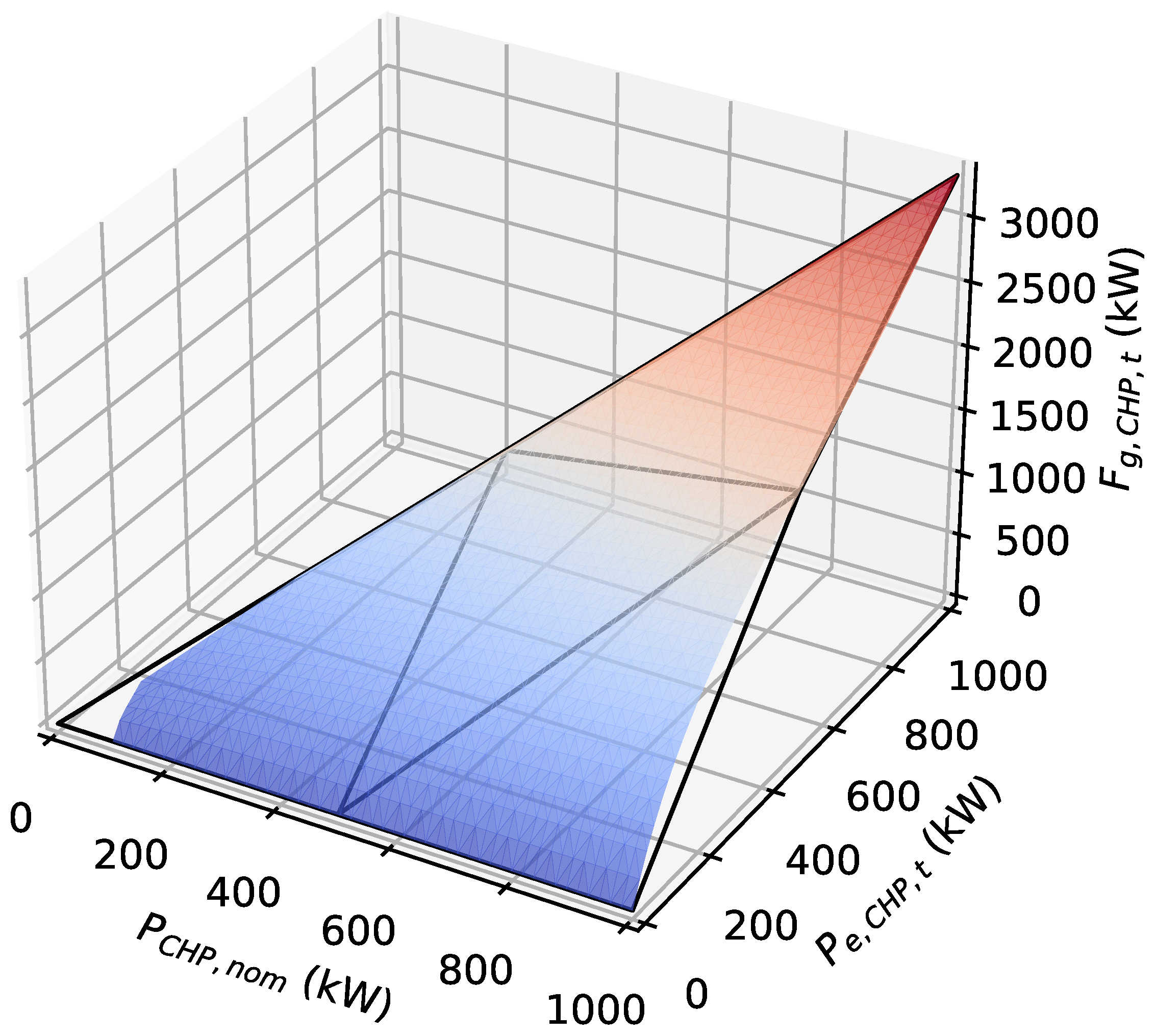
The second linearization method uses the technique from [28], also used to optimize an MES in [6], and which proposes piecewise linear approximations of functions of two variables. The so-called “triangle” method approximates the 2D function by the convex combination of triangles. This can be observed on Figure 2, where the colored surface represents the value of ${\mathit{F}}_{\mathit{g},\mathit{CHP},\mathit{t}}$ as a function of ${\mathit{P}}_{\mathit{e},\mathit{CHP},\mathit{t}}$ and ${\mathit{P}}_{\mathit{CHP},\mathit{nom}}$ (see Constraint (9)), and where four triangles approximate this surface. In this figure and the following ones, we consider values $P_{CHP,nom}^{min}=100 \mathrm{k}\mathrm{W}$ and $P_{CHP,nom}^{max}=1000 \mathrm{k}\mathrm{W}$ for these parameters.

To replace Constraint (9) with such an approximation, we need to introduce new parameters, new intermediate variables and new constraints to the model. Regarding the new parameters, let M (resp. N) represent the number of breakpoints along the ${\mathit{P}}_{\mathit{CHP},\mathit{nom}}$ (resp. ${\mathit{P}}_{\mathit{e},\mathit{CHP},\mathit{t}}$) axis (which will generate $M-1$ (resp. $N-1$) triangles). Let $x_m(m\in 1,\dots ,M)$ ($y_n(n\in 1,\dots ,N)$) be the breakpoints of the discretization along ${\mathit{P}}_{\mathit{CHP},\mathit{nom}}$ (resp. ${\mathit{P}}_{\mathit{e},\mathit{CHP},\mathit{t}}$). ${\mathit{P}}_{\mathit{e},\mathit{CHP},\mathit{t}}\le {\mathit{P}}_{\mathit{CHP},\mathit{nom}}$, as it is impossible to produce more than the nominal power of the CHP. As a consequence $M=N$.

The newly introduced variables are:

• ${\mathit{\alpha }}_{\mathit{m},\mathit{n},\mathit{t}}\in [0,1]$ which represent the coefficients of the convex combination $(\forall m=1,\dots ,M,n=1,\dots ,N,t\in \mathcal{T})$
• ${\mathit{h}}_{\mathit{m},\mathit{n},\mathit{t}}^{\mathit{u}}\in \{0,1\}$ and ${\mathit{h}}_{\mathit{m},\mathit{n},\mathit{t}}^{\mathit{l}}\in \{0,1\}$ that indicate which triangle is selected $(\forall m=1,\dots ,M-1,n=1,\dots ,N-1,t\in \mathcal{T})$

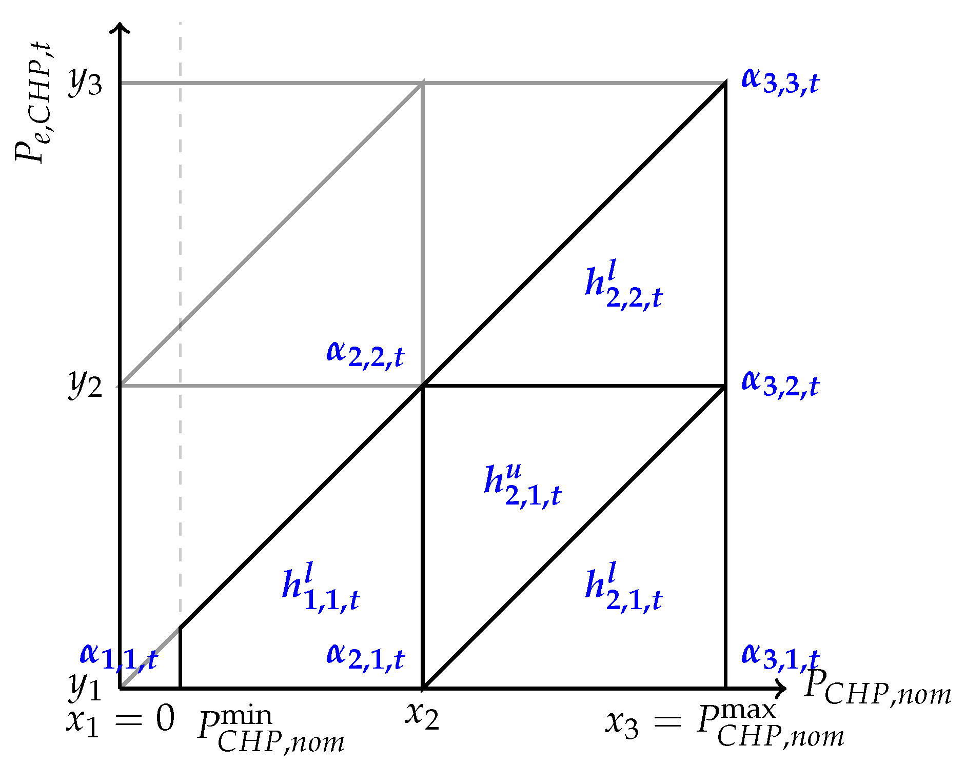
Figure 3 illustrate these variables (${\mathit{\alpha }}_{\mathit{m},\mathit{n},\mathit{t}}$, ${\mathit{h}}_{\mathit{m},\mathit{n},\mathit{t}}^{\mathit{u}}$ and ${\mathit{h}}_{\mathit{m},\mathit{n},\mathit{t}}^{\mathit{l}}$) and parameters (the breakpoints $x_m$ and $y_n$) for the case where N and M equal 3. From Constraint (9), the value of ${\mathit{F}}_{\mathit{g},\mathit{CHP},\mathit{t}}$ at the different breakpoints is given by the function:

$$f(x_m,y_n)=\frac{y_n}{a+b\left(\frac{y_n}{x_m}\right)+c{\left(\frac{y_n}{x_m}\right)}^2}\forall m=1,\dots ,M,\forall n\in 1,\dots ,N$$

(20)

On Figure 3 the gray triangles represent the part of the approximation which is not used here, as ${\mathit{P}}_{\mathit{e},\mathit{CHP},\mathit{t}}\le {\mathit{P}}_{\mathit{CHP},\mathit{nom}}$.

Constraint (9) is then replaced by the following new constraints:

$$\begin{array}{}\mathrm{(21a)}& {\sum }_{m=1}^M{\sum }_{n=1}^N{\mathit{\alpha }}_{\mathit{m},\mathit{n},\mathit{t}}=1\hfill & \hfill \forall t\in \mathcal{T}\mathrm{(21b)}& {\mathit{P}}_{\mathit{CHP},\mathit{nom}}={\sum }_{m=1}^M{\sum }_{n=1}^N{\mathit{\alpha }}_{\mathit{m},\mathit{n},\mathit{t}}{x}_m\hfill & \hfill \forall t\in \mathcal{T}\mathrm{(21c)}& {\mathit{P}}_{\mathit{e},\mathit{CHP},\mathit{t}}={\sum }_{m=1}^M{\sum }_{n=1}^N{\mathit{\alpha }}_{\mathit{m},\mathit{n},\mathit{t}}{y}_n\hfill & \hfill \forall t\in \mathcal{T}\mathrm{(21d)}& {\mathit{F}}_{\mathit{g},\mathit{CHP},\mathit{t}}={\sum }_{m=1}^M{\sum }_{n=1}^N{\mathit{\alpha }}_{\mathit{m},\mathit{n},\mathit{t}}f(x_m,y_n)\hfill & \hfill \forall t\in \mathcal{T}\mathrm{(21e)}& {\sum }_{m=1}^{M-1}{\sum }_{n=1}^{N-1}({\mathit{h}}_{\mathit{m},\mathit{n},\mathit{t}}^{\mathit{u}}+{\mathit{h}}_{\mathit{m},\mathit{n},\mathit{t}}^{\mathit{l}})=1\hfill & \hfill \forall t\in \mathcal{T}\mathrm{(21f)}& \begin{array}{c}{\mathit{\alpha }}_{\mathit{m},\mathit{n},\mathit{t}}\le {\mathit{h}}_{\mathit{m},\mathit{n},\mathit{t}}^{\mathit{u}}+{\mathit{h}}_{\mathit{m},\mathit{n},\mathit{t}}^{\mathit{l}}+{\mathit{h}}_{\mathit{m},\mathit{n}-\mathbf{1},\mathit{t}}^{\mathit{u}}+{\mathit{h}}_{\mathit{m}-\mathbf{1},\mathit{n}-\mathbf{1},\mathit{t}}^{\mathit{l}}\hfill \\ +{\mathit{h}}_{\mathit{m}-\mathbf{1},\mathit{n}-\mathbf{1},\mathit{t}}^{\mathit{u}}+{\mathit{h}}_{\mathit{m}-\mathbf{1},\mathit{n},\mathit{t}}^{\mathit{l}}\hfill \end{array}\hfill & \hfill \forall m\in 1,\dots ,M,\forall n\in 1,\dots ,N,\forall t\in \mathcal{T}\end{array}$$

Constraint (21a) ensures that the sum of all the coefficients ${\mathit{\alpha }}_{\mathit{m},\mathit{n},\mathit{t}}$ is equal to 1. Constraints (21b), (21c), and (21d) approximate the different variables of our model (${\mathit{P}}_{\mathit{CHP},\mathit{nom}}$, ${\mathit{P}}_{\mathit{e},\mathit{CHP},\mathit{t}}$, and ${\mathit{F}}_{\mathit{g},\mathit{CHP},\mathit{t}}$) using a convex combination. Constraint (21e) ensures that only one triangle is selected for the convex combination. Constraint (21f) makes sure that only the coefficients ${\mathit{\alpha }}_{\mathit{m},\mathit{n},\mathit{t}}$ associated with the selected triangle have a value different from 0. We consider dummy values of 0 at the extremes ($h_{0,\ast ,t}^{\ast }=h_{M,\ast ,t}^{\ast }=h_{\ast ,0,t}^{\ast }=h_{\ast ,N,t}^{\ast }=0$).

The resulting mathematical program is a mixed integer linear program (due to the newly introduced integer variables ${\mathit{h}}_{\mathit{m},\mathit{n},\mathit{t}}^{\mathit{u}}$ and ${\mathit{h}}_{\mathit{m},\mathit{n},\mathit{t}}^{\mathit{l}}$), which can be solved using classical mixed integer linear programming algorithms and solvers. However, compared to the linear program of the first method, we add $(M-1)·(N-1)·\left|\mathcal{T}\right|$ binary variables (or ${(N-1)}^2·\left|\mathcal{T}\right|$ since $M=N$) and $\left|\mathcal{T}\right|·(5+\frac{N(N+1)}{2})$ constraints, which clearly increases the complexity of the problem and therefore the calculation time to reach an optimal solution.

3.3. Proposed Adapted Piecewise Linearization Method

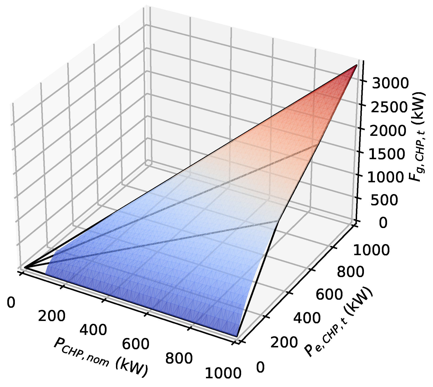
As a new variant of the classical piecewise linearization method, we propose an adapted linearization which introduces much less extra variables to the original model. The idea behind the proposed adapted linearization method is the fact that in the classical piecewise linearization method, nearly half of the triangles are not used in practice because of the particular shape of the surface representing ${\mathit{F}}_{\mathit{g},\mathit{CHP},\mathit{t}}$ (as it can be seen in Figure 3). We therefore propose to approximate this surface through fewer triangles, all having a vertex at the origin, as shown in Figure 4. Hereafter, we call the proposed method the “adapted method”.

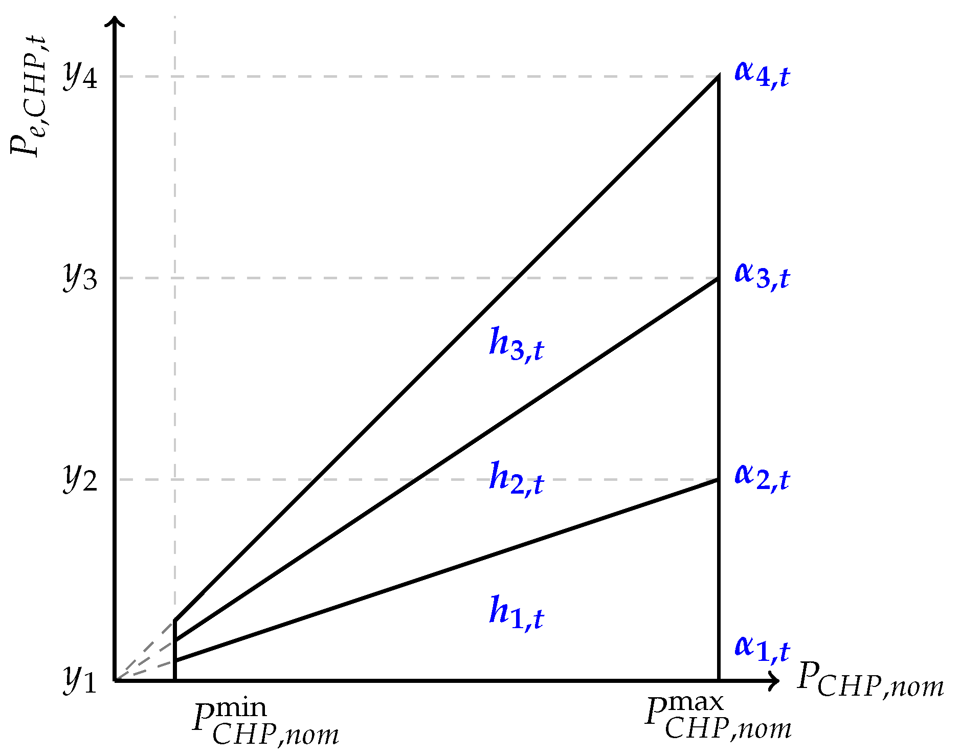
As it can be seen on Figure 5, the proposed method leads to introducing N breakpoints $y_n$ ($n\in 1,\dots ,N$) along the ${\mathit{P}}_{\mathit{e},\mathit{CHP},\mathit{t}}$ axis.

Consequently, we add the following variables to the original mathematical model of the MES:

• ${\mathit{\alpha }}_{\mathit{n},\mathit{t}}\in [0,1]$ ($\forall n\in 1,\dots ,N,t\in \mathcal{T}$)
• ${\mathit{h}}_{\mathit{n},\mathit{t}}\in \{0,1\}$ ($\forall n\in 1,\dots ,N-1,t\in \mathcal{T}$)

Constraint (9) is then replaced by the following new constraints:

$$\begin{array}{}\mathrm{(22a)}& {\sum }_{n=1}^N{\mathit{\alpha }}_{\mathit{n},\mathit{t}}\le 1\hfill & \hfill \forall t\in \mathcal{T}\mathrm{(22b)}& {\mathit{P}}_{\mathit{CHP},\mathit{nom}}={\sum }_{n=1}^N{\mathit{\alpha }}_{\mathit{n},\mathit{t}}{P}_{CHP,nom}^{max}\hfill & \hfill \forall t\in \mathcal{T}\mathrm{(22c)}& {\mathit{P}}_{\mathit{e},\mathit{CHP},\mathit{t}}={\sum }_{n=1}^N{\mathit{\alpha }}_{\mathit{n},\mathit{t}}{y}_n\hfill & \hfill \forall t\in \mathcal{T}\mathrm{(22d)}& {\mathit{F}}_{\mathit{g},\mathit{CHP},\mathit{t}}={\sum }_{n=1}^N{\mathit{\alpha }}_{\mathit{n},\mathit{t}}f(P_{CHP,nom}^{max},y_n)\hfill & \hfill \forall t\in \mathcal{T}\mathrm{(22e)}& {\sum }_{n=1}^{N-1}{\mathit{h}}_{\mathit{n},\mathit{t}}=1\hfill & \hfill \forall t\in \mathcal{T}\mathrm{(22f)}& {\alpha }_{\mathit{n},\mathit{t}}\le {\mathit{h}}_{\mathit{n},\mathit{t}}+{\mathit{h}}_{\mathit{n}-\mathbf{1},\mathit{t}}\hfill & \hfill \forall n\in 1,\dots ,N,\forall t\in \mathcal{T}\end{array}$$

Constraint (22a) ensures that the sum of all the coefficients ${\alpha }_{\mathit{n},\mathit{t}}$ is less or equal to 1. Constraints (22b), (22c), and (22d) approximate the different variables of our model (${\mathit{P}}_{\mathit{CHP},\mathit{nom}}$, ${\mathit{P}}_{\mathit{e},\mathit{CHP},\mathit{t}}$, and ${\mathit{F}}_{\mathit{g},\mathit{CHP},\mathit{t}}$) using a convex combination. Constraint (22e) ensures that only one triangle is selected for the convex combination. Constraint (22f) makes sure that only the coefficients ${\alpha }_{\mathit{n},\mathit{t}}$ associated with the selected triangle have a value different from 0. We consider dummy values of 0 at the extremes ($h_{0,t}=h_{N,t}=0$).

The resulting linearized mathematical model is still a mixed integer linear programming model (due to the integer variables ${\mathit{h}}_{\mathit{n},\mathit{t}}$). Compared to the first simplification method of Section 3.1, we add $(N-1)·\left|\mathcal{T}\right|$ binary variables and $\left|\mathcal{T}\right|·(5+N)$ constraints.

3.4. Multi-Objective Resolution

Finally, solving the original bi-objective mathematical model with the above-mentioned three simplification/linearization methods requires finding a set of non-dominated solutions, so-called Pareto solutions. Non-dominated Pareto solutions are the solutions from which none of them can be objectively preferred to another. Indeed, by switching between two non-dominated solutions, at least one objective is improved while (at least) another one deteriorates. To solve the linearized bi-objective model and to obtain non-dominated Pareto solutions, we use the $ϵ$-constraint method. First presented by [32], the $ϵ$-constraint method is used to transfer a multi-objective optimization model into a single-objective one, while still obtaining non-dominated Pareto solutions. In this method, one of the objectives is kept as the main objective function of the model, and the other objectives are transferred to the constraint body of the model by limiting the objectives with lower and upper bounds (i.e., value of $ϵ$) for minimization and maximization objectives, respectively. In our case, we optimize $ATCR$ (Objective (3)) while imposing an $ϵ$-constraint on ${\tau }_{RES}$ (Objective (4)).

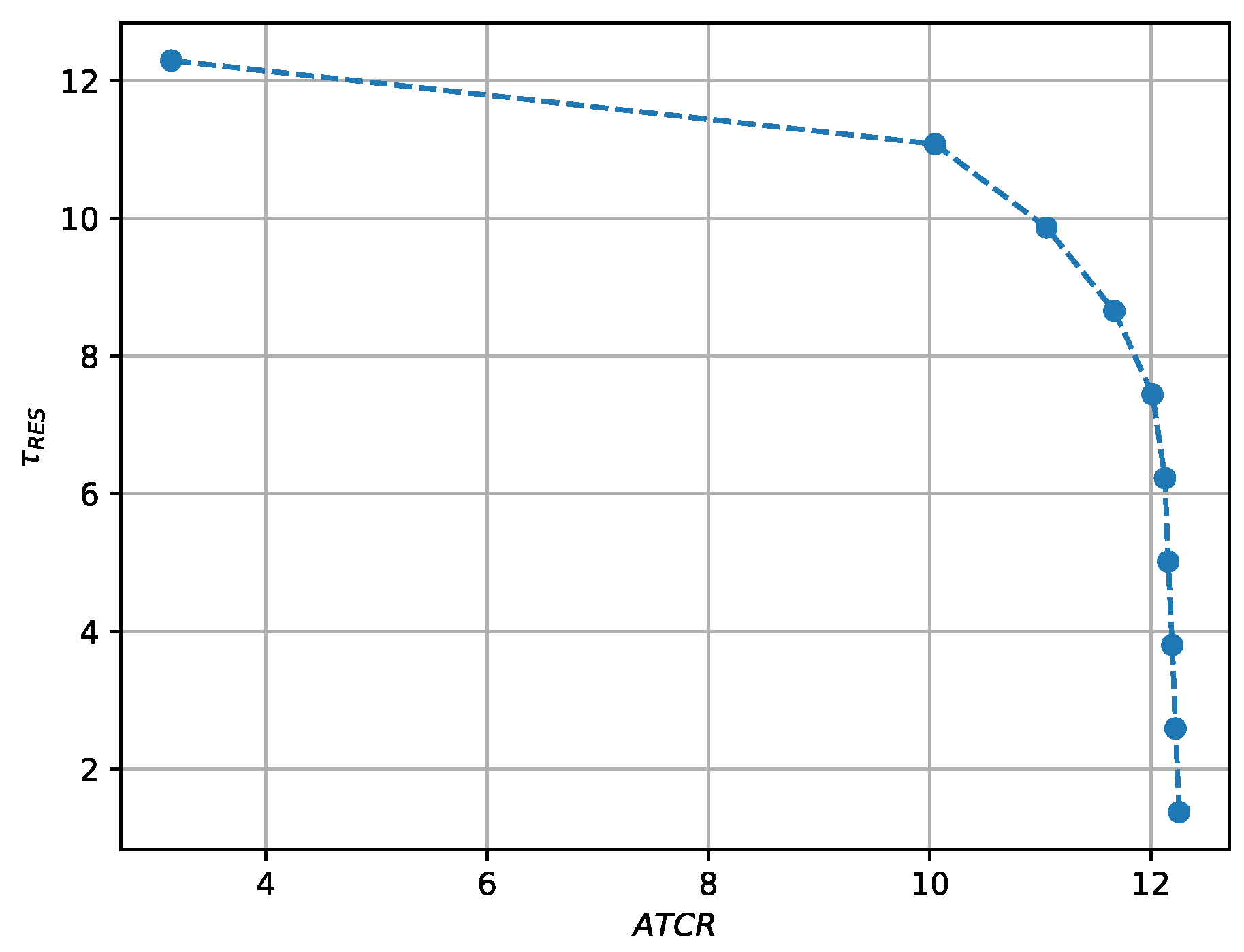
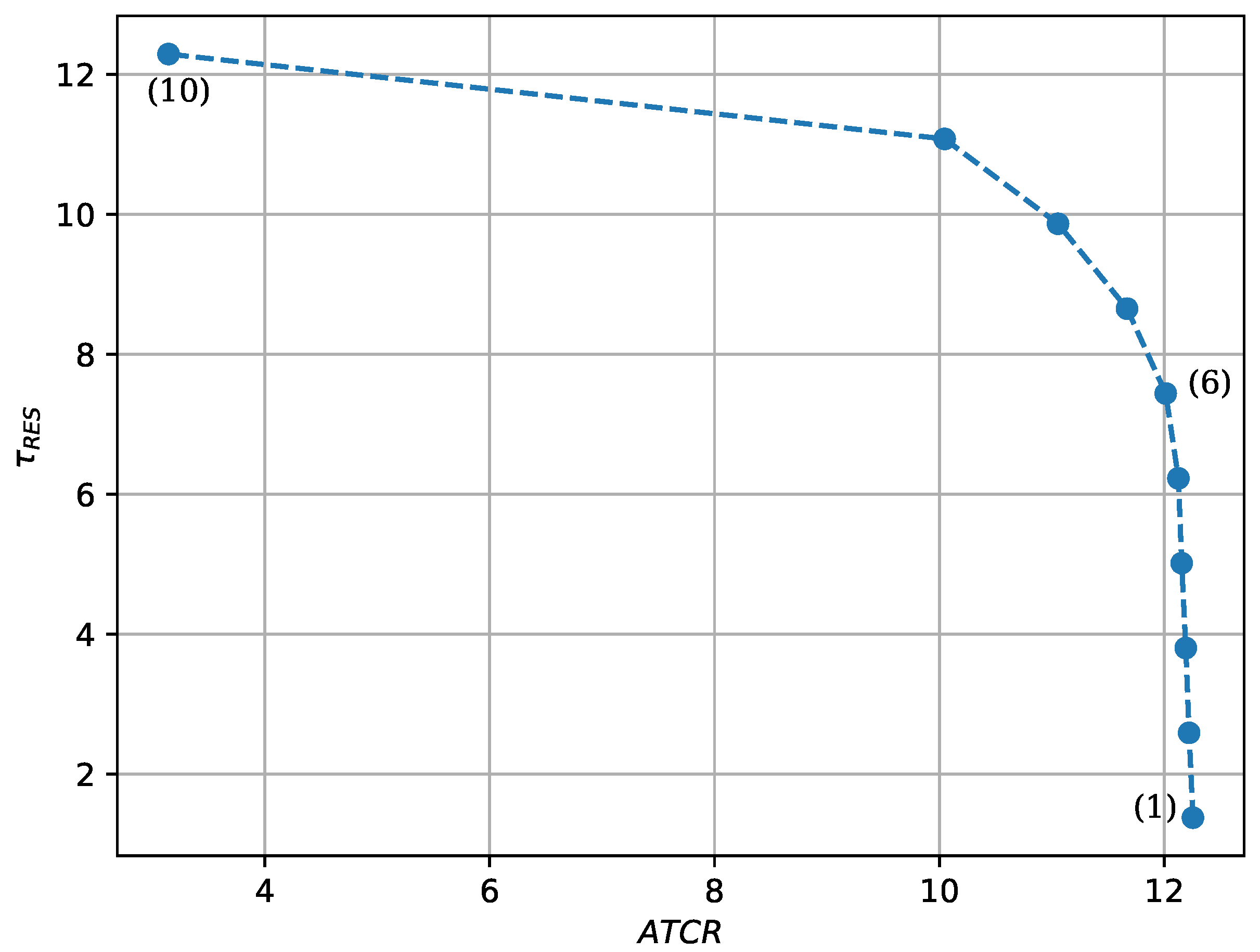
Figure 6 illustrates a Pareto front including ten non-dominated solutions of our mathematical model. The upper left solution maximizes the amount of energy produced by RES (and consequently is less interesting for the annual cost reduction objective), whereas the lower right solution maximizes the annual cost reduction (and is therefore less efficient in terms of RES usage). The remaining in-between solutions are intermediate Pareto-efficient configurations. An advantage of generating the set of Pareto solutions is that it provides more flexibility to the decision-maker when selecting a unique final solution among the Pareto set based on his/her preferences.

3.5. Discussion on the CHP Approximations

As explained in Section 2, we consider in this work that the CHP must be installed with a minimal capacity $P_{CHP,nom}^{min}$. The linearization methods proposed here can be coupled with other models to choose how many units of CHP are installed using other binary decision variables. The model proposed by [30] uses binary decision variables to decide how many units are installed and what size those units are, but does not take into account the non-linear part-load efficiency of the technologies. Their model, and subsequent work by [11], also allows using different efficiency functions for different installed capacities. However, the main difference with the approaches we present here is that these efficiency functions are always linear.

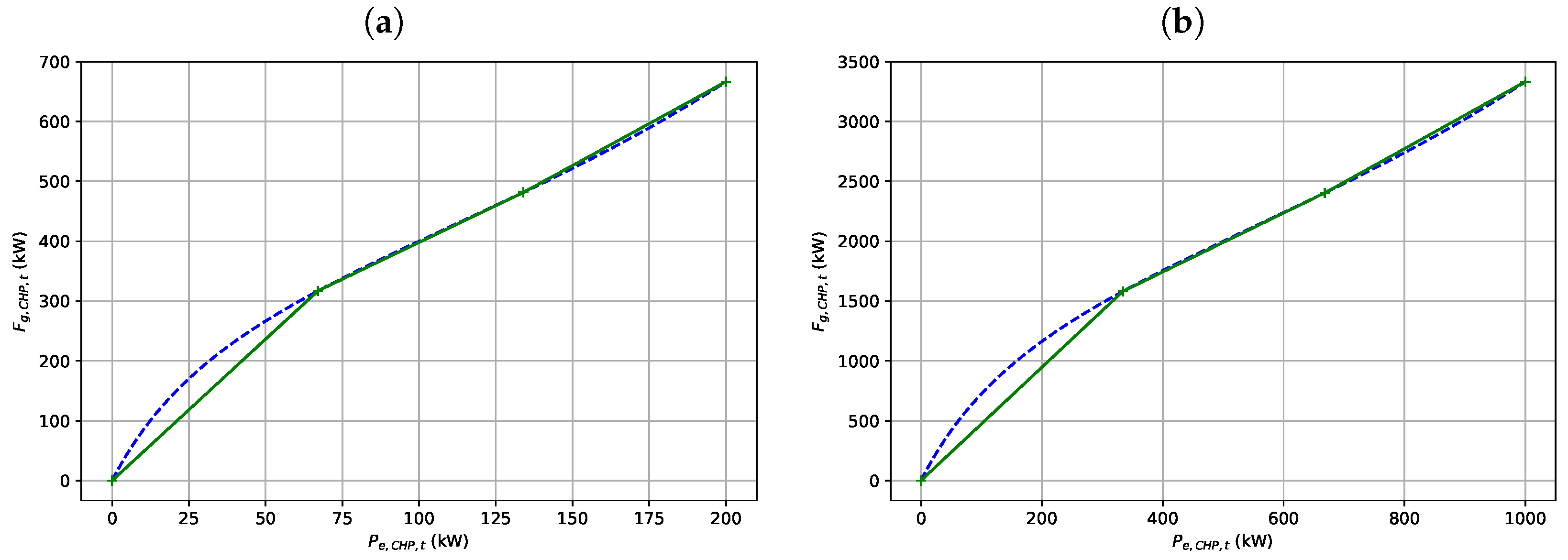
Figure 7 presents a view of the linearization method we propose in Section 3.3 for two different installed capacities (respectively $P_{CHP,nom}=200 \mathrm{k}{\mathrm{W}}_{\mathrm{e}}$ and $P_{CHP,nom}=1000 \mathrm{k}{\mathrm{W}}_{\mathrm{e}}$). On this figure, the blue dotted line represents the non-linear efficiency ${\eta }_{e,CHP,t}$ from Equation (10), and the plain green line represents the linearized approximation of this function with the proposed adapted piecewise method using three pieces. The methods used by [11,30] approximate the same efficiencies using a different linear function for each installed capacity for discrete installed capacities in [30] and for continuous capacities below or above a certain threshold in [11]. These functions are written as $P_{e,CHP,t}=k_1{F}_{g,CHP,t}+k_2{P}_{CHP,nom}+k_3$ with different coefficients $k_1$, $k_2$, and $k_3$ depending on the installed capacity. As can be seen in Figure 7, a purely linear function will not accurately approximate the real efficiency. We will also show in our results on a case study in Section 5.2 that such an approximated efficiency, represented by a linear function, significantly impacts the accuracy of the model.

Comparing the size of the two linearization approaches for the same number of breakpoints N along the ${\mathit{P}}_{\mathit{e},\mathit{CHP},\mathit{t}}$ axis, the method from the literature introduces $O(N^2·|\mathcal{T}\left|\right)$ binary variables and $O(N^2·|\mathcal{T}\left|\right)$ constraints in the model, while the proposed method introduces $O(N·|\mathcal{T}\left|\right)$ binary variables and $O(N·|\mathcal{T}\left|\right)$ constraints.

4. Case Study

In this section, a case study is presented, which will be used to validate the performances of the proposed resolution methods.

The case study represents an area in the vicinity of the city of Nantes in France. This area includes an MES, and it covers an area of 33.5 hectares, including the campus of IMT Atlantique, a French technological university, and 45 single-family houses [7]. The goal is to optimize the MES of the case study in terms of two objectives: (1) maximizing the rate of RES, and (2) maximizing the reduction of the costs of the system. The MES of the case study incorporates a set of available technologies: a combined heat and power unit, an electric boiler, a gas boiler, and photovoltaic as well as solar thermal panels.

Table 7. Cost (investment and operation) parameters per technology.

Technology j	${\mathit{\gamma }}_{\mathit{inv},\mathit{j}}$	${\mathit{\gamma }}_{\mathit{O}\&\mathit{M},\mathit{j},\mathit{f}}$	${\mathit{\gamma }}_{\mathit{O}\&\mathit{M},\mathit{j},\mathit{v}}$
$\mathit{CHP}$	1140 €/$\mathrm{k}$${\mathrm{W}}_{\mathrm{e}}$	-	21 €/$\mathrm{M}$${\mathrm{Wh}}_{\mathrm{e}}$
$\mathit{GB}$	90 €/$\mathrm{k}$${\mathrm{W}}_{\mathrm{th}}$	3.15 €/$\mathrm{k}$${\mathrm{W}}_{\mathrm{th}}$$\mathrm{year}$	-
$\mathit{EB}$	100 €/$\mathrm{k}$${\mathrm{W}}_{\mathrm{th}}$	1 €/$\mathrm{k}$${\mathrm{W}}_{\mathrm{th}}$$\mathrm{year}$	0.8 €/$\mathrm{M}$${\mathrm{Wh}}_{\mathrm{th}}$
$\mathit{PV}$	1000 €/$\mathrm{k}$${\mathrm{W}}_{\mathrm{e}}$	15 €/$\mathrm{k}$${\mathrm{W}}_{\mathrm{e}}$$\mathrm{year}$	-
$\mathit{ST}$	615 €/$\mathrm{m}$${}^2$	10 €/$\mathrm{m}$${}^2$$\mathrm{year}$	-

and

Table 8. General parameters of the case study.

Parameter	Description
$P_{CHP,nom}^{min}=100 \mathrm{k}{\mathrm{W}}_{\mathrm{e}}$, $P_{CHP,nom}^{max}=1000 \mathrm{k}{\mathrm{W}}_{\mathrm{e}}$	Minimum and maximum nominal power of the CHP
$P_{GB,nom}^{min}=100 \mathrm{k}{\mathrm{W}}_{\mathrm{th}}$, $P_{GB,nom}^{max}=3000 \mathrm{k}{\mathrm{W}}_{\mathrm{th}}$	Minimum and maximum nominal power of the GB
$P_{EB,nom}^{min}=100 \mathrm{k}{\mathrm{W}}_{\mathrm{th}}$, $P_{EB,nom}^{max}=3000 \mathrm{k}{\mathrm{W}}_{\mathrm{th}}$	Minimum and maximum nominal power of the EB
$A_{PV}^{min}=0 {\mathrm{m}}^2$, $A_{PV}^{max}=\text{10,000} {\mathrm{m}}^2$	Minimum and maximum area of the PV panels
$A_{ST}^{min}=0 {\mathrm{m}}^2$, $A_{ST}^{max}=\text{10,000} {\mathrm{m}}^2$	Minimum and maximum area of the ST panels
$L_{e,t}$ ($\mathrm{k}{\mathrm{W}}_{\mathrm{e}}$)	Electricity demand of the system
$L_{h,t}$ ($\mathrm{k}{\mathrm{W}}_{\mathrm{th}}$)	Heat demand of the system
$a=0.1$, $b=0.4$, $c=-0.2$	Electrical efficiency coefficients of the CHP
$\beta =0.3$	Constant CHP electrical efficiency
${\eta }_{th,CHP}=0.8$	Thermal efficiency of the heat recuperation system of the CHP
${\eta }_{GB}=0.8$	Efficiency of the GB
${\eta }_{EB}=0.8$	Efficiency of the EB
${\eta }_{DC/AC}=0.9$	PV inverters’ efficiency
${\eta }_{ref}=0.155$	Reference efficiency for PV
$G_{\beta ,t}$ ($\mathrm{W}/{\mathrm{m}}^{-2}$)	Global solar radiation
$\alpha =0.43\%{/}^{\circ }\mathrm{C}$	Temperature coefficient of PV
$T_{ref}=25{}^{\circ }\mathrm{C}$	Reference temperature
$T_{a,t}$ (${}^{\circ }\mathrm{C}$)	Outdoor temperature
$P_{panel,nom}=250 \mathrm{W}$	Nominal power of a PV panel
$A_{panel}=1.6 {\mathrm{m}}^2$	Area of a PV panel
${\eta }_0=0.8$	Optical efficiency of ST
$U_{loss}=5 \mathrm{W}/{\mathrm{m}}^{-2}{/}^{\circ }{\mathrm{C}}^{-1}$	Thermal loss coefficient of ST
$T_{w,m}=45 {}^{\circ }\mathrm{C}$	Mean water temperature in the ST collector
$A_{total}=\text{10,000} {\mathrm{m}}^2$	Total area available for solar panels
$C_{gr,t}$ = 0.13 €/$\mathrm{k}$$\mathrm{Wh}$	Cost of electricity bought from the grid (0 h–7 h)
$C_{gr,t}$ = 0.17 €/$\mathrm{k}$$\mathrm{Wh}$	Cost of electricity bought from the grid (8 h–23 h)
$C_g$ = 0.076 €/$\mathrm{k}$$\mathrm{Wh}$	Cost of gas bought
$I_{gr}$ = 0.1 €/$\mathrm{k}$$\mathrm{Wh}$	Price of electricity sold to the grid

present a summary of the values of the parameters used in this case study. The investment and operation and maintenance costs of the technologies come from [33] for the GB, ref. [34] for the EB, ref. [35] for the PV panels, and [7] for the CHP and ST panels. The different costs of electricity ($C_{gr,t}$ and $I_{gr}$) and gas ($C_g$) are the market price in France, from EDF in October 2021. The other parameters in Table 8 are from [7].

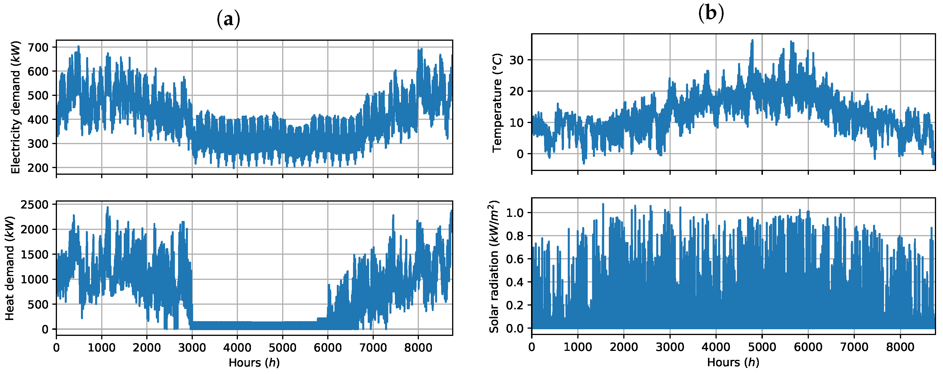
In Table 8, some of the parameters ($L_{e,t}$, $L_{h,t}$, $G_{\beta ,t}$, and $T_{a,t}$) are time series and are presented in Figure 8. Figure 8a presents the energy demands of the system: the electricity demand $L_{e,t}$ and the heat demand $L_{h,t}$. They are represented as a time series over the year with an hourly resolution. These are a mix of real and simulated data. Measured electricity and heat consumption monthly data are available for the campus buildings, and they are disaggregated into hourly time series. For the electricity demand, it was considered that the studied area is representative to the region’s electrical consumption, and the electricity demand of the region was scaled accordingly to match the yearly consumption of the campus buildings. The hourly heat demand of the campus is produced from the monthly data using a degree-hour method. The data for the 45 houses are generated using TRNSYS simulation software version 18 (http://www.trnsys.com/, accessed on 5 October 2023) to model residential houses complying with the RT2012 French thermal regulations [7]. The total energy demands over the year are 3.6 GWh and 6.1 GWh for electricity and heat, respectively. Figure 8b presents the environmental parameters: the outdoor temperature $T_{a,t}$ and the global solar radiation $G_{\beta ,t}$. These two parameters are used in the calculation of the energy generated by RES.

5. Experimentation

This section presents the experiments used to study the proposed resolution methods. First, the experimental design and the performance indicators are presented; second, the results are analyzed from a numerical and from an energy point of view.

5.1. Experimental Design

The purpose of this study is to compare the three resolution methods in terms of approximation quality and computation time. We study also the impact of the number of triangles on the quality of the solution for the triangle method (i.e., the classical piecewise linearization method of Section 3.2) and our proposal (i.e., the proposed adapted piecewise linearization method of Section 3.3). This will allow us to choose a resolution method adapted to our problem. Next to that, it is also interesting to study the impact of the chosen method on the physical characteristics of the solutions which are obtained when solving the problem.

To conduct this study, we need to solve the optimization problem at hand a large number of times (for each resolution method and each number of triangles). However, the resolution of the problem for the whole considered year is very time-consuming (in the order of days, even for low numbers of triangles). Therefore, to be able to carry out the numerous calculations in a reasonable time, we decide to study in a first stage three typical weeks of the considered year. This reduces the calculation time significantly, and allows us to solve multiple problems to optimality in a reasonable amount of time. The chosen weeks are one week in winter (days 45 to 52 of the year), one week in summer (days 164 to 171), and finally one week at mid-season (days 262 to 269). This allows to assess the resolution methods and the effect of the linearization on three different demand profiles. The mean value and standard deviation of the energy demands and environmental parameters are presented in

Table 9. Energy demands and environmental parameters of the three weeks.

	${\mathit{L}}_{\mathit{e},\mathit{t}}$	${\mathit{L}}_{\mathit{h},\mathit{t}}$
Summer	$\mu =322 \mathrm{kW}$, $\sigma =54 \mathrm{kW}$	$\mu =55 \mathrm{kW}$, $\sigma =58 \mathrm{kW}$
Mid-season	$\mu =337 \mathrm{kW}$, $\sigma =55 \mathrm{kW}$	$\mu =395 \mathrm{kW}$, $\sigma =390 \mathrm{kW}$
Winter	$\mu =526 \mathrm{kW}$, $\sigma =82 \mathrm{kW}$	$\mu =1459 \mathrm{kW}$, $\sigma =528 \mathrm{kW}$
	${\mathit{T}}_{\mathit{t}}$	${\mathit{G}}_{\mathit{\beta },\mathit{t}}$
Summer	$\mu =15.1 °\mathrm{C}$, $\sigma =2.8 °\mathrm{C}$	$\mu =175 \mathrm{W} {\mathrm{m}}^{-2}$, $\sigma =214 \mathrm{W} {\mathrm{m}}^{-2}$
Mid-season	$\mu =16.5 °\mathrm{C}$, $\sigma =4.5 °\mathrm{C}$	$\mu =196 \mathrm{W} {\mathrm{m}}^{-2}$, $\sigma =279 \mathrm{W} {\mathrm{m}}^{-2}$
Winter	$\mu =5.4 °\mathrm{C}$, $\sigma =4.6 °\mathrm{C}$	$\mu =123 \mathrm{W} {\mathrm{m}}^{-2}$, $\sigma =224 \mathrm{W} {\mathrm{m}}^{-2}$

. In summer, there is a low power demand and a very low heat demand. During the mid-season week, the energy demands are higher and more fluctuating, and there is a higher potential for RES from the environmental parameters (temperature and solar radiation). In winter, there is a high energy demand and low values for the environmental parameters.

To validate that the conclusions of the selected resolution method on the above three weeks can be extrapolated to the whole year, we also study the influence of the number of triangles on the recommended resolution method on the whole year. Again, as this potentially requires a long computation time, we decide to stop the resolution when the gap to the optimal solution is sufficiently small on each of the objective functions. We set the optimality gap to 0.1%. This small gap is negligible based on the expertise of energy specialists.

To evaluate the impact of the number of triangles on the two linearization methods, we test each of them with different numbers of triangles. For the triangle method, the number of triangles varies from $1^2$, $2^2$, …, $6^2$ (when possible in less than 10⁵ s), and for the adapted method, the number of triangles varies from 1, …, 36 (when possible in less than 10⁵ s ). For each resolution, a set of Pareto-optimal solutions $\mathcal{S}$ is obtained using the $ϵ$-constraints method. Furthermore, we use three different performance indicators for these tests: the computation time, the mean distance of the Pareto front to the origin to evaluate the evolution of the Pareto fronts with the number of triangles, and a measure of the approximation error. The computation time for one resolution is given by the sum of the computation times of all the $\left|\mathcal{S}\right|$ steps of the $ϵ$-constraints method.

The evolution of the positions of the Pareto fronts (or rather of their calculated representative solutions) with respect to the number of breakpoints can be seen through the mean Euclidean distance to the origin for the $\left|\mathcal{S}\right|$ solutions s of $\mathcal{S}$:

$$\mathit{mean}\mathit{distance}=\frac{1}{\left|\mathcal{S}\right|}\sum _{s\in \mathcal{S}}\sqrt{{{\mathit{ATCR}}^s}^2+{{\tau }_{RES}^s}^2}$$

(23)

This mean distance should change with the number of triangles, and when its value stabilizes in our experiments for some iterations (i.e., changes in the number of triangles), this indicates that the position of the Pareto front remains stable for these numbers of triangles and there is no need to still increase the number of triangles.

The mean cumulative error is calculated as the mean of the errors of the elements s of $\mathcal{S}$, as presented in Equation (24). The error of s is the sum across the different time steps of the absolute value of the difference between the approximated value ${\mathit{F}}_{\mathit{g},\mathit{CHP},\mathit{t}}^{\mathit{s}}$ and the real function $f(x,y)=\frac{y}{a+b\left(\frac{y}{x}\right)+c{\left(\frac{y}{x}\right)}^2}$ for the same (approximate) values of ${\mathit{P}}_{\mathit{CHP},\mathit{nom}}^{\mathit{s}}$ and ${\mathit{P}}_{\mathit{e},\mathit{CHP},\mathit{t}}^{\mathit{s}}$.

$$\mathit{mean}\mathit{cumulative}\mathit{error}=\frac{1}{\left|\mathcal{S}\right|}\sum _{s\in \mathcal{S}}\sum _{t\in \mathcal{T}}|{\mathit{F}}_{\mathit{g},\mathit{CHP},\mathit{t}}^{\mathit{s}}-f({\mathit{P}}_{\mathit{CHP},\mathit{nom}}^{\mathit{s}},{\mathit{P}}_{\mathit{e},\mathit{CHP},\mathit{t}}^{\mathit{s}})|$$

(24)

If the mean cumulative error is close to 0, the difference between the approximation and the real consumption f is small, and the approximation can be considered as optimal.

5.2. Results

All the models were solved using the Gurobi solver version 9.5 (https://www.gurobi.com/, accessed on 5 October 2023) on a computation server, using 400 GB RAM and Intel Xeon Gold 6138 @ 2.00 GHz CPUs, with 32 threads as recommended by the Gurobi documentation.

The next section will present numerical results for the three proposed weeks in winter, summer, and at mid-season, as well as results over the full year.

5.2.1. Numerical Analysis

Figure 9 shows the mean cumulative error for each week, calculated using Equation (24). The abscissa represents the number of triangles in the linearization methods.

The method with a constant efficiency is represented on the figures by a single point that we placed on the value of 0 triangles, since this method doesn’t involve any linearization. For the two linearization methods, we can see that, depending on the week, the error decreases before reaching a constant value when the number of triangles increases.

In summer, Figure 9a shows that for the adapted method (depicted by the orange curve), the error decreases rapidly with an increase of the number of triangles. However, for the triangle method from the literature (depicted by the green line), the error remains constant. To understand these phenomena, we must determine on which part of the curve of Equation (20) we are located. In summer, there is less demand of energy, the CHP is therefore less used and the value of the variable ${\mathit{P}}_{\mathit{CHP},\mathit{nom}}$ is always equal to $P_{CHP,nom}^{min}$. Hence ${\mathit{P}}_{\mathit{e},\mathit{CHP},\mathit{t}}\le P_{CHP,nom}^{min}$. On Figure 10, line (a) represents the part of the function to be approximated for the summer week. As can be seen in this figure, to decrease the error for the values on this line, the number of triangles of the triangle method must be quite high, i.e., higher than $P_{CHP,nom}^{max}/{\mathit{P}}_{\mathit{CHP},\mathit{nom}}=1000/100=10$ on each axis. As a consequence, for this resolution method, more than 100 triangles are needed to influence the approximation in that area of the surface. However, using so many triangles would make the computation time very high.On the contrary, the approximation of this line is impacted by the triangles of the adapted method, as soon as the number of triangles is greater or equal to 2, as it can easily be seen on Figure 4.

In the mid-season week on Figure 9b, we can see that the error for the triangle method (green line) stays stable from 1 to 9 triangles, with a slight increase in the error at 4 triangles, and starts decreasing when there are more than 9 triangles. This can be explained for the same reason as previously, via line (b) of Figure 10. ${\mathit{P}}_{\mathit{CHP},\mathit{nom}}$ is on average 301 kW over the $\left|\mathcal{S}\right|$ solutions at mid-season, so we would need more than $P_{CHP,nom}^{max}/{\mathit{P}}_{\mathit{CHP},\mathit{nom}}=1000/301\approx 3.3$ triangles on each axis (or more than 9 triangles in total) to see a change in the error. The decrease in the error is therefore visible starting from 16 triangles. For the adapted method, the error decreases very quickly with the number of triangles increasing, and seems to stabilize after 10 to 15 triangles. We suppose that the error of the triangle method will probably decrease to the same error as the adapted one, but very high calculation times prevent us to demonstrate it.

For the winter week on Figure 9c, the two linearization methods have a similar behavior. This is again due to the part of the function that is approximated, which is represented in Figure 10 by line (c). ${\mathit{P}}_{\mathit{CHP},\mathit{nom}}$ is on average 560 kW over the $\left|\mathcal{S}\right|$ solutions, and as expected, both linearization methods impact this part of the function even with small numbers of triangles. However, the adapted method decreases more rapidly and stabilizes after approximately 10 to 15 triangles.

The study of the results for this first indicator show that the proposed adapted method is much more efficient to reduce the error between the real function and the approximation, for each of the three weeks. Next to that, a choice of 9 triangles for this method seems to be adequate, as no significant improvement can be observed above that number.

Figure 11 represents the mean distances for each week, calculated using Equation (23). Again, the abscissa represents the number of triangles of the linearization method, with the value of 0 used to indicate the method with the constant efficiency where there is no linearization. We can see that the values of the mean distances follow approximately the same trend as the mean distance error values, except during the winter week, where the mean distance moves around the same value of 13.545, which indicates that the Pareto front doesn’t evolve.

The mean distance to the origin decreases (or stays roughly constant) when the number of triangles increases, which means that the set of Pareto-optimal solutions (and thus the Pareto front) moves towards the origin. These movements are however not due to the same causes. Figure 12 shows, for each week, the variations of the average values of the two objective functions taken separately across the Pareto fronts ($ATCR$ on the left, and ${\tau }_{RES}$ on the right). More precisely, each point represents the average value of the objective functions across the $\left|\mathcal{S}\right|=10$ Pareto optimal solutions, and the error bar represents the corresponding standard deviation. For instance, we can see that for the summer and the mid-season weeks and the adapted linearization method, the $ATCR$ objective varies more than the ${\tau }_{RES}$ objective, with respect to the number of triangles. In winter, the average values of both objectives in the Pareto fronts show very small variations when the number of triangles changes. The variations of the two objective functions within the same Pareto front are on the other hand quite constant, as a function of the number of triangles, in the three weeks. However, when we compare the three weeks between them, these variations are very different. In summer (resp. mid-season), for $ATCR$, the Pareto fronts are quite narrow, with a standard deviation of about $\sigma =0.022$ (resp. 0.035), whereas for winter the front is much wider, with a standard deviation of about 2.7. For ${\tau }_{RES}$, we can observe similar phenomena, with rather narrow Pareto fronts in summer ($\sigma =0.29$) and mid-season ($\sigma =0.33$), and a wide one for winter ($\sigma =3.68$). It is also interesting to note that the variations of both objective functions across the Pareto fronts do not seem to be influenced by the number of triangles, for any of the methods.

These distance plots of Figure 11 show again that the adapted method causes the Pareto front to converge more quickly than the triangle method, with respect to the number of triangles. Again, a choice of 9 triangles for the adapted method seems to be adequate, as no significant changes in the Pareto front can be observed above that value.

Figure 13 represents the computation time (seconds on a logarithmic scale) for the three resolution methods when the number of triangles increases. As expected with the analysis of the number of integer variables used by each solving method (see Section 3), the adapted method requires significantly less computation time than the triangle method. Obviously, the constant method requires the shortest computation time, as no integer variables are introduced in this case.

As can be seen on these figures, the proposed linearization method requires much less computation time, by a factor of about 10, than the method from the literature for an equivalent number of piecewise linear triangles. We can also see that the computation times required are different for the three periods analyzed, with the mid-season week (Figure 13b) requiring computation times 10 to 100 times longer than the other periods (Figure 13a,c).

If we consider the analyses of the error and distance indicators together with the calculation time, we can see that for a given number of triangles, the error measure and the calculation time speak in favor of the adapted resolution method. These analyses lead us to conclude that the adapted resolution method seems to be the most appropriate method for these three weeks. Therefore, we apply it to the whole year. First trial and error experiments show that it is nearly impossible to solve this problem to optimality, even with a small number of triangles. As mentioned in the experimental design section, we therefore stop the resolution when the gap to the optimal solution is small on each of the objective functions, with a gap value of 0.1%.

Figure 14 shows the three indicators, mean cumulative error, mean distance and computation time for the adapted method for the full year. First of all, we observe similar phenomena as for the three selected weeks. The error decreases when the number of triangles increases, and the mean distance indicator and the values of the objective functions stabilize with a higher number of triangles. We can also observe that the computation time increases with the number of triangles. Optimizing the system with the proposed adapted method required 2.3 × 10⁶ s (i.e., 26 days) over the full year with 15 triangles, whereas it required at most 3.3 × 10³ s (i.e., 55 min) over one week for the same number of triangles. In addition, it was not possible to solve the system with more than one triangle using the literature method.

Let us now switch to the questions linked to the physical impact of these optimizations.

5.2.2. Energy Analysis

Figure 15 shows the boxplot of the efficiency of the CHP ${\eta }_{e,CHP,t}={\mathit{P}}_{\mathit{e},\mathit{CHP},\mathit{t}}/{\mathit{F}}_{\mathit{g},\mathit{CHP},\mathit{t}}$, from Constraint (9), for each of the $\left|\mathcal{S}\right|=10$ solutions of the Pareto front, for each of the three weeks. The values where ${\mathit{F}}_{\mathit{g},\mathit{CHP},\mathit{t}}=0$ are ignored. From Equation (10) and according to the parameters of our case study from Table 8, we know that ${\eta }_{e,CHP,t}\in [0.1,0.3]$. We can see that for the mid-season and the winter weeks, the median efficiency is close to the maximum value of 0.3. However, this means that during those two weeks, the CHP runs half of the time only at a partial load and a good approximation of its efficiency is therefore important. For the summer week, ${\eta }_{e,CHP,t}$ is at most equal to $0.27$. It shows that the CHP always run at a partial load, therefore, ${\mathit{P}}_{\mathit{CHP},\mathit{nom}}=100$ and ${\mathit{P}}_{\mathit{e},\mathit{CHP},\mathit{t}}<100(\forall t\in \mathcal{T})$ according to our parameters from Table 8. A constant efficiency of 0.3 is therefore not accurate, especially for the summer week.

Table 10. Output percentages of the technologies for the adapted method with 9 triangles.

Run	${\mathit{P}}_{\mathit{e},\mathit{CHP}}$	${\mathit{P}}_{\mathit{e},\mathit{PV}}$	${\mathit{U}}_{\mathit{e}}$	${\mathit{P}}_{\mathit{h},\mathit{CHP}}$	${\mathit{P}}_{\mathit{h},\mathit{GB}}$	${\mathit{P}}_{\mathit{h},\mathit{EB}}$	${\mathit{P}}_{\mathit{h},\mathit{ST}}$	$\mathit{ATCR}$	${\mathit{\tau }}_{\mathit{RES}}$
Summer (1)	7%	$49.6\%$	$43.4\%$	$99.9\%$	$0.1\%$	0%	0%	34.47	42.43
Summer (6)	$6.4\%$	$50.2\%$	$43.4\%$	$94.4\%$	$5.5\%$	$0.1\%$	0%	34.46	42.91
Summer (10)	$6.3\%$	$50.4\%$	$43.2\%$	$92.7\%$	$5.3\%$	$1.9\%$	0%	34.41	43.29
Mid-season (1)	$42.2\%$	$41.5\%$	$16.2\%$	$69.3\%$	$30.5\%$	$0.2\%$	0%	27.57	18.87
Mid-season (6)	$41.1\%$	$42.7\%$	$16.2\%$	$67.2\%$	$32.5\%$	$0.2\%$	0%	27.55	19.40
Mid-season (10)	$40.6\%$	$43.3\%$	$16.1\%$	$67.2\%$	32%	$0.8\%$	0%	27.45	19.83
Winter (1)	$93.8\%$	$5.2\%$	1%	65%	35%	0%	0%	12.26	1.38
Winter (6)	$71.4\%$	$27.6\%$	1%	52%	$47.5\%$	$0.5\%$	0%	12.01	7.44
Winter (10)	$77.9\%$	$18.6\%$	$3.5\%$	$55.2\%$	$34.7\%$	$0.1\%$	10%	3.14	12.29

shows the contribution (%) of each technology to the energy generation for the adapted linearization method with 9 triangles. For each week, 10 solutions, numbered from (1) to (10), are calculated on the Pareto front. Three of these solutions are displayed in the tables: solutions (1) correspond to the maximization of the cost reduction, solutions (10) correspond to the maximization of the rate of RES, and solutions (6) correspond to an intermediate solution in the Pareto front, as shown as an example for the winter week on Figure 16. The last two columns show the value of the two objective functions for each solution.

Regarding the optimization over the year,

Table 11. Output energy of the technologies for the adapted method with 15 triangles.

Run	${\mathit{P}}_{\mathit{e},\mathit{CHP}}$	${\mathit{P}}_{\mathit{e},\mathit{PV}}$	${\mathit{U}}_{\mathit{e}}$	${\mathit{V}}_{\mathit{e}}$	${\mathit{P}}_{\mathit{h},\mathit{CHP}}$	${\mathit{P}}_{\mathit{h},\mathit{GB}}$	${\mathit{P}}_{\mathit{h},\mathit{EB}}$	${\mathit{P}}_{\mathit{h},\mathit{ST}}$	$\mathit{ATCR}$	${\mathit{\tau }}_{\mathit{RES}}$
Year (1)	2.02 GWh	840 MWh	701 MWh	1.14 GWh	4.05 GWh	2.02 GWh	1.54 MWh	0 Wh	15.71	8.73
Year (6)	1.69 GWh	1.22 GWh	698 MWh	755 MWh	3.44 GWh	2.59 GWh	45 MWh	0 Wh	15.51	12.68
Year (10)	1.75 GWh	1.2 GWh	769 MWh	310 MWh	3.55 GWh	2.07 GWh	129 MWh	322 MWh	4.48	15.84

shows the total energy generated over the year by each technology for the adapted method with 15 triangles and a gap of 0.1% for the solver. We can see that regardless of the solution s of the Pareto front $\mathcal{S}$, the CHP generates most of the energy over the year. Thus, a good approximation of the performance of the CHP seems important to accurately represent the system. This also impacts the other technologies and the amount of electricity $U_e$ and $V_e$ bought and sold to the grid.

Table 12. Output energy of the technologies for the method with constant efficiency.

Run	${\mathit{P}}_{\mathit{e},\mathit{CHP}}$	${\mathit{P}}_{\mathit{e},\mathit{PV}}$	${\mathit{U}}_{\mathit{e}}$	${\mathit{V}}_{\mathit{e}}$	${\mathit{P}}_{\mathit{h},\mathit{CHP}}$	${\mathit{P}}_{\mathit{h},\mathit{GB}}$	${\mathit{P}}_{\mathit{h},\mathit{EB}}$	${\mathit{P}}_{\mathit{h},\mathit{ST}}$	$\mathit{ATCR}$	${\mathit{\tau }}_{\mathit{RES}}$
Year (1)	2.22 GWh	760 MWh	576 MWh	1.22 GWh	4.15 GWh	1.91 GWh	1.31 MWh	0 Wh	16.14	7.89
Year (6)	1.82 GWh	1.18 GWh	578 MWh	791 MWh	3.39 GWh	2.66 GWh	16.4 MWh	0 Wh	16.00	12.31
Year (10)	1.88 GWh	1.19 GWh	642 MWh	299 MWh	3.51 GWh	2.1 GWh	124 MWh	335 MWh	4.32	15.84

shows the total energy generated over the year by each technology when considering a constant efficiency ${\eta }_{e,CHP,t}$. We can observe similar tendencies as in Table 11, but with different values. For example, there is a relative difference of 9% for $P_{e,CHP}$ between the constant and the adapted method in these results for the solution (1). We can also observe a difference in the values of the objective functions between Table 11 and Table 12. The relative difference of $ATCR$ varies between 2.7% and 3.7%, while the relative difference of ${\tau }_{RES}$ varies between 0% and 10.6% for solutions (10) and (1), respectively.

Figure 17 shows the boxplot of the efficiency of the CHP ${\eta }_{e,CHP,t}$ over the year. This figure shows that the CHP runs close to its rated power half of the time, the median value of ${\eta }_{e,CHP,t}$ being close to 0.3, which is the maximum efficiency of the CHP with the parameters used in this case study. However, we can also see that the other half of the time the CHP runs at a partial load.

Figure 18 represents the energy outputs for two days of the year, from hours 6400 to 6448. The MES has been optimized over the full year with a gap of 0.1%, and we focus only over two days of the year to have a detailed view on the operation of the MES. Figure 18a–c represent three solutions (1), (6), and (10) from the set of 10 solutions, respectively. The figures on the left depict the power energy, and those on the right represent the heat energy. On these figures, the blue area represents the energy output of the CHP with the proposed adapted linearization method, and the other colored areas represent the energy output of the other technologies. The blue dotted line represents the energy output of the CHP with a constant efficiency ${\eta }_{CHP,t}$, as a comparison. Finally, the black line represents the energy demands; the power demand ($L_{e,t}$) on the left and the heat demand ($L_{h,t}$) on the right. The black dashed line on the electricity figures represents the extra power required for the EB.

We can observe that there is a difference between ${\mathit{P}}_{\mathit{e},\mathit{CHP},\mathit{t}}$ and ${\mathit{P}}_{\mathit{h},\mathit{CHP},\mathit{t}}$ using a linearized efficiency (blue areas) and ${\mathit{P}}_{\mathit{e},\mathit{CHP},\mathit{t}}$ and ${\mathit{P}}_{\mathit{h},\mathit{CHP},\mathit{t}}$ using a constant efficiency (blue dotted lines). Over the two days represented on the figures, ${\mathit{P}}_{\mathit{e},\mathit{CHP},\mathit{t}}$ is overestimated when using a constant efficiency compared to the more precise linearized efficiency. Consequently, according to Equation (11), ${\mathit{P}}_{\mathit{h},\mathit{CHP},\mathit{t}}$ is underestimated when using a constant efficiency. We observe that the linearization method modifies the energy produced by the CHP, and therefore also modifies the energy produced by other technologies to meet the energy demand. For example, around hour 6440 in Figure 18a, the GB is used to produce a part of the heat when a linearization method is used, while only the CHP is used if a constant efficiency is considered. Therefore, the use of a linearization method seems more appropriate to better represent the system.

Regarding the different solutions, we can see an evolution in the usage of the EB, around hour 6440, between Figure 18a–c. For solution (1) (Figure 18a), when we maximize $ATCR$, the EB is not used at all. However, when we increase the RES usage according to the second objective function ${\tau }_{RES}$, a part of the electricity is used to produce heat through the EB instead of being sold to the grid. When we maximize ${\tau }_{RES}$ in solution (10) (Figure 18c), we can see that ST panels are installed and they produce heat in contrary to the other solutions. However, PV panels produce less power in this solution. Most of the heat of ST is wasted on the two days presented here, but for other parts of the year, the ST panels are used more efficiently. Moreover, the CHP is limited by both the electricity and the heat demands. Taking into account multiple energy vectors in an MES is therefore important to optimize the system.

6. Conclusions and Perspectives

6.1. Summary of the Contributions

In this paper, we have modeled the design and the operation of an MES as a non-linear mathematical optimization program, summarized in Table 6. Our study has shown that a classical linearization method from the literature shows its limits when it comes to optimizing the problem on a full year period. Because of the specific shape of the CHP efficiency function, we have adapted the classical linearization method of the literature by proposing a linearization method introducing much fewer decision variables, which allows us to solve the optimization problem on a full year, with an optimality gap of 0.1%.

6.2. Discussion

We observe that the obtained solutions are faithful to reality. Whether it is on the three weeks that we have chosen to determine the interest of our linearization method, or on the whole year, we can see that the implemented techniques are well dimensioned and allow for answering the energy demand. In contrast to what one could expect, in all the obtained Pareto solutions, the solar panels appear each time at maximum surface. This is directly linked to their cost, which allows them to be used in all circumstances.

The results of our experiments on typical weeks show that the proposed adapted method requires a shorter computation time and less linearization pieces than the method from the literature for a similar quality. The proposed method requires about 10 times less computation time than the literature method for the same number of piecewise linear triangles, and the approximation error decreases much faster with regard to the number of triangles when using the proposed method. On the contrary, the approximation error decreases slower or even remains constant when using the classical linearization method, meaning that a higher number of triangles is needed for this method to accurately approximate the non-linear function. For a similar computation time of 5 × 10⁴ s, the adapted method’s error is 80% lower than the method from the literature. The analysis for a full year confirms these results. Even by allowing an optimality gap when obtaining the solutions, it has not been possible to solve the model with the method from the literature for more than a single triangle per variable, while the adapted method solved the model with up to 15 triangles. Comparing the energy over the year of the proposed linearized method and the simplified constant method, we can see a relative difference of 9% in the output power of the CHP, and up to 10.6% relative difference in the values of the objective functions, showing that a more accurate approximation yields more realistic solutions to the optimization problem.

A set of analyses showed that having multiple energy vectors in an MES is an advantage to globally optimize the system. The operation of the CHP is based on both the power and the heat demand, and the energy produced by a technology can be used to power another technology, as presented on the example of the PV panels and the EB (please see Figure 18). Furthermore, the CHP provides most of the heat and power to respond to the demands, up to 93.8% of the power during the winter week, and up to 99.9% of heat during the summer week (please see Table 10).

Having two objective functions is also interesting in the optimization process, as we observed that the different solutions of the Pareto front can be very different from each other. We have also investigated how the non-linearities affect differently different solutions.

6.3. Limitations and Perspectives

The proposed method gives a lower approximation error than the literature method in a faster computation time, making it possible to optimize an MES over a full year. However, this method is not without its limitations. It cannot be generalized to all two-variable functions, as it assumes that all piecewise linear triangles have a common vertex at the origin, which simplifies the model by removing a large number of decision variables compared to a traditional linearization method. In addition, computation times remain high, with resolution over the year requiring 2.3 × 10⁶ s to optimize the MES with an optimality gap of 0.1%. A possible improvement to the proposed linearization method would be to choose more carefully the location of the breakpoints used for linearization, so as to have more breakpoints where the function is less linear, and fewer breakpoints where it is more linear.

Although this study obtains a set of Pareto optimal solutions, the problem is not yet completely solved for a real decision maker. In fact, there are a set of solutions among which the decision maker must choose the configuration that corresponds best to his/her preferences. One of the perspectives of our work could be integrating preference models in the multi-objective optimization via an interactive method. Accordingly, the optimization process is guided using the decision-maker’s preferences toward a most preferred optimal solution.

In this work, we also simplified the problem by setting investment costs proportional to the installed capacity. However, in reality, these costs are often modeled as non-linear functions since a larger installed capacity is proportionally less expensive than a smaller capacity [11]. Hence, another perspective of this work is then to take into account these non-linear costs using a piecewise linear approximation for a more realistic model.

Another simplification is the use of a single unit for each technology. In most real-world settings, multiple units are available, and a part of the design of an MES is to optimize the number of units installed. This would introduce other integer variables in the model to decide how many units of each type are installed. Therefore, making decisions on the use of multiple units for each technology could be another possible perspective of this work. The full-load efficiency is also simplified in this model. We consider that the full-load efficiency is linear with regard to the installed capacity. In most CHP units, a higher capacity would have a better full-load efficiency. Refs. [11,30] model this problem by using different linear efficiency functions for different installed capacities. Our proposed adapted piecewise linearization approach could be coupled with these models to allow different non-linear efficiency functions for different unit capacities.

Last but not least, energy storage has not been considered in this work. However, this topic is of a crucial importance and should be integrated in the system modeling to avoid energy losses. We therefore plan to integrate storage solutions in our model, which will be represented by non-linear constraints, and will probably require approximate optimization methods for their resolution.

References

1. Shabanpour-Haghighi, A.; Karimaghaei, M. An overview on multi-carrier energy networks: From a concept to future trends and challenges. Int. J. Hydrog. Energy 2022, 47, 6164–6186. [Google Scholar] [CrossRef]
2. Beigvand, S.D.; Abdi, H.; Scala, M.L. Multicarrier energy systems. In Handbook of Energy Economics and Policy; Academic Press: Cambridge, MA, USA, 2021; pp. 433–519. [Google Scholar] [CrossRef]
3. Alabi, T.M.; Agbajor, F.D.; Yang, Z.; Lu, L.; Ogungbile, A.J. Strategic potential of multi-energy system towards carbon neutrality: A forward-looking overview. Energy Built Environ. 2023, 4, 689–708. [Google Scholar] [CrossRef]
4. Ghanbari, A.; Karimi, H.; Jadid, S. Optimal planning and operation of multi-carrier networked microgrids considering multi-energy hubs in distribution networks. Energy 2020, 204, 117936. [Google Scholar] [CrossRef]
5. Fonseca, J.D.; Commenge, J.M.; Camargo, M.; Falk, L.; Gil, I.D. Multi-criteria optimization for the design and operation of distributed energy systems considering sustainability dimensions. Energy 2021, 214, 118989. [Google Scholar] [CrossRef]
6. Bischi, A.; Taccari, L.; Martelli, E.; Amaldi, E.; Manzolini, G.; Silva, P.; Campanari, S.; Macchi, E. A detailed MILP optimization model for combined cooling, heat and power system operation planning. Energy 2014, 74, 12–26. [Google Scholar] [CrossRef]
7. Adihou, Y.; Mabrouk, M.T.; Haurant, P.; Lacarrière, B. A multi-objective optimization model for the operation of decentralized multi-energy systems. J. Phys. Conf. Ser. 2019, 1343, 012104. [Google Scholar] [CrossRef]
8. Geidl, M.; Andersson, G. Optimal Power Flow of Multiple Energy Carriers. IEEE Trans. Power Syst. 2007, 22, 145–155. [Google Scholar] [CrossRef]
9. Li, K.; Ding, Y.Z.; Ai, C.; Sun, H.; Xu, Y.P.; Nedaei, N. Multi-objective optimization and multi-aspect analysis of an innovative geothermal-based multi-generation energy system for power, cooling, hydrogen, and freshwater production. Energy 2022, 245, 123198. [Google Scholar] [CrossRef]
10. Wu, M.; Du, P.; Jiang, M.; Goh, H.H.; Zhu, H.; Zhang, D.; Wu, T. An integrated energy system optimization strategy based on particle swarm optimization algorithm. Energy Rep. 2022, 8, 679–691. [Google Scholar] [CrossRef]
11. Gabrielli, P.; Gazzani, M.; Martelli, E.; Mazzotti, M. Optimal design of multi-energy systems with seasonal storage. Appl. Energy 2018, 219, 408–424. [Google Scholar] [CrossRef]
12. Weber, C.I. Multi-Objective Design and Optimization of District Energy Systems Including Polygeneration Energy Conversion Technologies. Ph.D. Thesis, École Polytechnique Fédérale de Lausanne, Lausanne, Switzerland, 2008. [Google Scholar] [CrossRef]
13. Shan, J.; Lu, R. Multi-objective economic optimization scheduling of CCHP micro-grid based on improved bee colony algorithm considering the selection of hybrid energy storage system. Energy Rep. 2021, 7, 326–341. [Google Scholar] [CrossRef]
14. Zhao, Y.; Zhou, M.; Yue, Z.; Tan, T.; Zheng, M. Prospective optimization of CCHP system under multi-scenarios. Energy Rep. 2022, 8, 952–958. [Google Scholar] [CrossRef]
15. Fazlollahi, S.; Mandel, P.; Becker, G.; Maréchal, F. Methods for multi-objective investment and operating optimization of complex energy systems. Energy 2012, 45, 12–22. [Google Scholar] [CrossRef]
16. Wirtz, M.; Hahn, M.; Schreiber, T.; Müller, D. Design optimization of multi-energy systems using mixed-integer linear programming: Which model complexity and level of detail is sufficient? Energy Convers. Manag. 2021, 240, 114249. [Google Scholar] [CrossRef]
17. Mancarella, P. MES (multi-energy systems): An overview of concepts and evaluation models. Energy 2014, 65, 1–17. [Google Scholar] [CrossRef]
18. Piacentino, A.; Cardona, F. EABOT—Energetic analysis as a basis for robust optimization of trigeneration systems by linear programming. Energy Convers. Manag. 2008, 49, 3006–3016. [Google Scholar] [CrossRef]
19. Yousefi, H.; Ghodusinejad, M.H.; Noorollahi, Y. GA/AHP-based optimal design of a hybrid CCHP system considering economy, energy and emission. Energy Build. 2017, 138, 309–317. [Google Scholar] [CrossRef]
20. Poncelet, K.; Delarue, E.; Six, D.; Duerinck, J.; D’haeseleer, W. Impact of the level of temporal and operational detail in energy-system planning models. Appl. Energy 2016, 162, 631–643. [Google Scholar] [CrossRef]
21. Salpakari, J.; Mikkola, J.; Lund, P.D. Improved flexibility with large-scale variable renewable power in cities through optimal demand side management and power-to-heat conversion. Energy Convers. Manag. 2016, 126, 649–661. [Google Scholar] [CrossRef]
22. Milan, C.; Stadler, M.; Cardoso, G.; Mashayekh, S. Modeling of non-linear CHP efficiency curves in distributed energy systems. Appl. Energy 2015, 148, 334–347. [Google Scholar] [CrossRef]
23. Teichgraeber, H.; Brandt, A.R. Time-series aggregation for the optimization of energy systems: Goals, challenges, approaches, and opportunities. Renew. Sustain. Energy Rev. 2022, 157, 111984. [Google Scholar] [CrossRef]
24. Puchinger, J.; Raidl, G.R. Combining Metaheuristics and Exact Algorithms in Combinatorial Optimization: A Survey and Classification. In Artificial Intelligence and Knowledge Engineering Applications: A Bioinspired Approach; Springer: Berlin/Heidelberg, Germany, 2005; pp. 41–53. [Google Scholar] [CrossRef]
25. Fischetti, M.; Fischetti, M. Matheuristics. In Handbook of Heuristics; Martí, R., Pardalos, P.M., Resende, M.G.C., Eds.; Springer: Cham, Switzerland, 2018; pp. 121–153. [Google Scholar] [CrossRef]
26. Tesio, U.; Guelpa, E.; Verda, V. Including thermal network operation in the optimization of a Multi Energy System. Energy Convers. Manag. 2023, 277, 116682. [Google Scholar] [CrossRef]
27. Raidl, G.R.; Puchinger, J. Combining (Integer) Linear Programming Techniques and Metaheuristics for Combinatorial Optimization. In Hybrid Metaheuristics; Springer: Berlin/Heidelberg, Germany, 2008; pp. 31–62. [Google Scholar] [CrossRef]
28. D’Ambrosio, C.; Lodi, A.; Martello, S. Piecewise linear approximation of functions of two variables in MILP models. Oper. Res. Lett. 2010, 38, 39–46. [Google Scholar] [CrossRef]
29. Kotzur, L.; Nolting, L.; Hoffmann, M.; Groß, T.; Smolenko, A.; Priesmann, J.; Büsing, H.; Beer, R.; Kullmann, F.; Singh, B.; et al. A modeler’s guide to handle complexity in energy systems optimization. Adv. Appl. Energy 2021, 4, 100063. [Google Scholar] [CrossRef]
30. Yokoyama, R.; Shinano, Y.; Taniguchi, S.; Ohkura, M.; Wakui, T. Optimization of energy supply systems by MILP branch and bound method in consideration of hierarchical relationship between design and operation. Energy Convers. Manag. 2015, 92, 92–104. [Google Scholar] [CrossRef]
31. Klemm, C.; Vennemann, P. Modeling and optimization of multi-energy systems in mixed-use districts: A review of existing methods and approaches. Renew. Sustain. Energy Rev. 2021, 135, 110206. [Google Scholar] [CrossRef]
32. Haimes, Y.Y. Integrated System Identification and Optimization. In Control and Dynamic Systems; Academic Press: Cambridge, MA, USA, 1973; Volume 10, pp. 435–518. [Google Scholar] [CrossRef]
33. Gudmundsson, O.; Thorsen, J.E.; Zhang, L. Cost analysis of district heating compared to its competing technologies. In Proceedings of the WIT Transactions on Ecology and the Environment, Bucharest, Romania, 19–21 June 2013; WIT Press: Southampton, UK, 2013; Volume 176, pp. 3–13. [Google Scholar] [CrossRef]
34. Armila, N. Electrification as an Alternative for Combustion Technologies in Existing Finnish District Heating Networks. Master’s Thesis, Aalto University, School of Electrical Engineering, Espoo, Finland, 2020. [Google Scholar]
35. Ashfaq, A.; Ianakiev, A. Cost-minimised design of a highly renewable heating network for fossil-free future. Energy 2018, 152, 613–626. [Google Scholar] [CrossRef]
Figure 1. Technologies in the multi-energy system.
Mathematics 11 04855 g001
Figure 2. Visualization of the linearization with 2 × 2 triangles.
Mathematics 11 04855 g002
Figure 3. Top view of the linearization with 2 × 2 triangles.
Mathematics 11 04855 g003
Figure 4. Visualization of the linearization with 3 pieces.
Mathematics 11 04855 g004
Figure 5. Top view of the linearization with 3 pieces.
Mathematics 11 04855 g005
Figure 6. 10 solutions of a Pareto front.
Mathematics 11 04855 g006
Figure 7. Adapted piece-wise linearization for two different installed capacities. (a) Installed capacity P C H P , n o m = 200   k W e . (b) Installed capacity P C H P , n o m = 1000   k W e .
Mathematics 11 04855 g007
Figure 8. Time series parameters: (a) energy demands ( L e , t , L h , t ) and (b) environmental parameters ( T a , t , G β , t ).
Mathematics 11 04855 g008
Figure 9. Mean cumulative errors for the (a) summer week, (b) mid-season week and (c) winter week.
Mathematics 11 04855 g009
Figure 10. Parts of the function to be approximated for the three weeks: (a) summer, (b) mid-season and (c) winter.
Mathematics 11 04855 g010
Figure 11. Mean distances for the (a) summer week, (b) mid-season week and (c) winter week.
Mathematics 11 04855 g011
Figure 12. Objective functions (average and standard deviation) for the (a) summer week, (b) mid-season week (c) and winter week.
Mathematics 11 04855 g012
Figure 13. Computation times for the (a) summer week, (b) mid-season week (c) and winter week.
Mathematics 11 04855 g013
Figure 14. Indicators on the full year (gap 0.1%): (a) mean cumulative errors, (b) mean distances, (c) computation times and (d) objective functions.
Mathematics 11 04855 g014
Figure 15. Efficiency η e , C H P for 10 solutions using the adapted method with 9 triangles, for the (a) summer week, (b) mid-season week and (c) winter week.
Mathematics 11 04855 g015
Figure 16. Three solutions of the Pareto front for the winter week.
Mathematics 11 04855 g016
Figure 17. Efficiency η e , C H P for the adapted method with 15 triangles over the year.
Mathematics 11 04855 g017
Figure 18. Outputs for two days of the year for the adapted linearization method with 15 triangles: (a) solution (1), (b) solution (6), (c) solution (10).
Mathematics 11 04855 g018