Queueing-Inventory Systems with Catastrophes under Various Replenishment Policies

Abstract

We discuss two queueing-inventory systems with catastrophes in the warehouse. Catastrophes occur according to the Poisson process and instantly destroy all items in the inventory. The arrivals of the consumer customers follow a Markovian arrival process and they can be queued in an infinite buffer. The service time of a consumer customer follows a phase-type distribution. The system receives negative customers which have Poisson flows and as soon as a negative customer comes into the system, he causes a consumer customer to leave the system, if any. One of two inventory policies is used in the systems: either $(s,S)$ or $(s,Q)$. If the inventory level is zero when a consumer customer arrives, then this customer is either lost (lost sale) or joins the queue (backorder sale). The system is formulated by a four-dimensional continuous-time Markov chain. Ergodicity condition for both systems is established and steady-state distribution is obtained using the matrix-geometric method. By numerical studies, the influence of the distributions of the arrival process and the service time and the system parameters on performance measures are deeply analyzed. Finally, an optimization study is presented in which the criterion is the minimization of expected total costs and the controlled parameter is warehouse capacity.

1. Introduction

Until the early 1990s of the last century, in the theory of operations research, models of queuing systems (QS) and models of inventory control systems (ICS) were studied separately. In other words, it was believed that in ICS there is no server for releasing items to consumers (i.e., a self-service rule is used), and in QS, only an idle server is required to service customers (i.e., no additional items are required). However, in real ICSs, the release of items to consumer customers (c-customers) requires the presence of a service station in which the incoming c-customer is processed, and the processing time is often a positive random variable. A classic example of such systems is the widespread systems of gas stations. These ICSs with positive service time can also be considered as QSs, in which in order to service c-customers, in addition to an idle server, a positive level of certain inventory is required. Note that ICSs with positive service time are called queuing-inventory systems (QIS) in [1,2]. However, QIS models were first proposed earlier in [3,4] and have been intensively studied by various authors over the past three decades. For a detailed overview of known results on QIS models, see [5,6,7].

To classify QISs models, their various properties can be taken as a basis. Based on the type of QIS model being studied, the lifetime of the system’s inventory is taken as the basis for the classification. The vast majority of work on QIS assumes that the system’s inventory never deteriorates. However, in real situations, system inventories often lose their quality over time and after a certain time (deterministic or random) they become unsuitable for use. Such systems are called systems with perishable inventory and have been studied in detail in numerous works, see, for example, [8,9,10,11,12,13,14,15,16]. Note that inventory damage can occur instantly as a result of some accidents, like power outage, equipment failures, staff negligence, etc. A sequence of accidents can be considered as an arrival of destructive customers.

QIS models with destructive customers hardly have been studied, although, as indicated above, they are accurate models of systems in real life. In papers [17,18,19,20], the authors assumed that the arrival of destructive customers causes the level of the inventory is reduced only by one. However, there are many realistic QISs in which upon arrival of destructive customers all items damage together. Below this type of systems is called QISs with catastrophes in warehouse. It is necessary to distinguish between models of QIS with catastrophes in the warehouse and models of QIS with common lifetime (e.g., foods or medicines with the same expiry date), see [21,22,23,24,25,26,27]. In models of QISs with common lifetime, it is assumed that all items in the warehouse have the same age at any given time. In other words, all items of inventory is considered arrived by one batch of orders. However, in the model of QIS with catastrophes in the warehouse, this assumption is not required. Note that similar models of QS (but not QIS) with catastrophes are widely investigated in available literature. In lieu of reviewing work related to models of QS with catastrophes, we highlight representative papers [28,29,30,31,32,33,34] and refer readers to their reference lists. In QS, disaster events immediately destroy the system. Namely, all customers waiting in the queue and obtaining service are removed from the system.

To increase the adequacy of the QIS model under study to real situations, we also take into account the possibility of negative customers (n-customers) arriving at the service station. Negative customers can be interpreted as customers that agitate c-customers in the system so that they do not buy the inventory in that system. In other words, n-customers do not require the inventory, but their arrival force one c-customer leaves the system.

One of the main shortcomings of the known works devoted to QIS is that they analyze models with either backorders or lost sales, i.e., QIS models that simultaneously use both backorders and lost sales are practically not considered. However, in realistic QIS an arrived c-customer either joins the queue (backorder) or loses the system without inventory (lost sale) if upon its arrival an inventory level is zero, i.e., the hybrid sale rule is frequently used in realistic QISs. Regardless of popularity, models of QISs with hybrid sales are poorly understood due to their complexity.

Ref. [35] first studied the model of single-server perishable QIS (without destructive customers) with a capacited waiting room under $(s,Q)$, $Q=S-s>s+1$, inventory policy. They assumed that both types of c-customers and n-customers arrive in the system according to a Markovian arrival process and the service time of c-customers, lead time and lifetime of each item have exponential distributions with finite means; an n-customer at an arrival epoch removes the random number of waiting c-customers. The authors obtained the joint probability distribution of the number of c-customers in the system and the inventory level. A similar double sources model of QIS was considered in a recent paper [36].

The motivation for this study is that models of QIS with warehouse catastrophes under realistic assumptions have been practically unstudied. In a recent paper [37] assumed that all kinds of customers arrived according to independent Poisson processes and all other underlying random variables to be exponentially distributed (Poisson/exponential assumptions); authors studied models in steady-state under various replenishment policies. This paper is a continuation of the research begun in [37] under more realistic assumptions related to system operation, i.e., here we assume that c-customers arrive according to $MAP$, n-customers arrive according to a Poisson process, the service times to be of phase-type distribution ($PH$-distribution), and lead times to be exponentially distributed. Under these assumptions, we use matrix-analytic methods to analyze the QISs with catastrophes in a warehouse under two replenishment policies: $(s,S)$ and $(s,Q)$ policies. Note that the indicated replenishment policies are defined as follows. In both policies, it is assumed that the warehouse capacity is S, $S<\infty$, and the reorder level is s, $s<S$, and a replenishment order is not offered if the current (observed) inventory level is more than s. In an $(s,Q)$ policy, the order size is fixed and equal to $Q=S-s$. In this case, the constraint on the value of s is defined as follows: $s<Q$. This constraint is accepted to avoid perpetual order placement for replenishment. However, in an $(s,S)$ policy, the order size is variable, i.e., here replenishment size is that much to bring the inventory level to S at the replenishment epoch. In policy $(s,S)$ there are no restrictions on the value of s, as in policy $(s,Q)$, i.e., here the parameter s can take any value from 0 to $S-1$.

More specifically, the main differences between our model and the model considered in known works are as follows: (i) we consider model of QISs with catastrophes in warehouse; (ii) the model with infinite queue for c-customers is investigated; (iii) service time of c-customers have phase time ($PH$) distribution; (iv) only c-customers represents $MAP$ flow; (v) hybrid sale rule is used, i.e., some customers may join the queue (backorder scheme) or be lost (lose sale scheme) according to the Bernoulli scheme if the inventory level is zero at the time of their arrival.

The paper is organized as follows. In Section 2 the proposed queueing-inventory system is exhaustively described. Section 3 shows the structure of the generator matrices for the underlying processes and provides the steady-state analysis of the systems. That is, Section 3.1 includes matrices and analysis for the model-1 under $(s,S)$-policy, and Section 3.2 includes ones for the model-2 under $(s,Q)$-policy. Expressions for various essential performance measures to assess both system efficiencies are formulated in Section 4. Section 5 presents a numerical analysis to highlight separately the qualitative behaviour of the queueing-inventory system under each inventory policy; the effect of the system parameters on the performance measures under various arrival process and service time distribution in Section 5.1 and optimization study for the each inventory policy in Section 5.2. Finally, concluding remarks are given in Section 6.

At this point, we define some notation for use in the sequel. $\mathit{e}$ is a unit column vector; ${\mathit{e}}_j$ is a unit column vector of dimension j; ${\mathit{e}}_j\left(i\right)$ is a unit column vector with 1 in the ith position and 0 elsewhere and ${\mathit{I}}_k$ is an identity matrix of order k. The symbols ⊗ and ⊕ represent the Kronecker product and the Kronecker sum, respectively. If $\mathit{A}$ is a matrix of order $m\times n$ and if $\mathit{B}$ is a matrix of order $p\times q$, then the Kronecker product of the two matrices is given by $\mathit{A}\otimes \mathit{B}$, a matrix of order $mp\times nq$; the Kronecker sum of two square matrices, say, $\mathit{G}$ of order g and $\mathit{H}$ of h, is given by $\mathit{G}\oplus \mathit{H}=\mathit{G}\otimes {\mathit{I}}_h+{\mathit{I}}_g\otimes \mathit{H}$, a square matrix of order $gh$. The transpose notation is denoted by ${}^{\prime }$.

2. Model Description

We analyze a queueing-inventory system with negative customers and catastrophes in the warehouse as demonstrated in Figure 1.

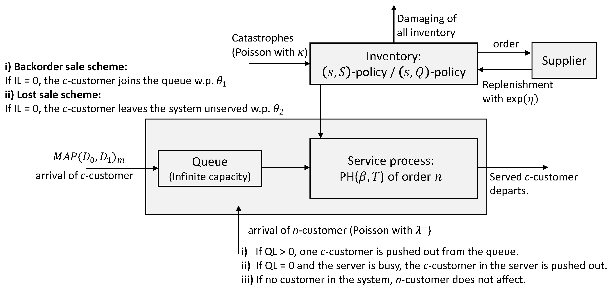
• The c-customers (consumer customers) arrive in the system according to the Markovian arrival process ($MAP$) with representation ${({\mathit{D}}_0,{\mathit{D}}_1)}_m$. The underlying Markov chain of the $MAP$ is governed by the matrix $\mathit{D}$$(={\mathit{D}}_0+{\mathit{D}}_1)$. Such that, the entries of matrix ${\mathit{D}}_0$ denote the transition rates without arrival while the entries of matrix ${\mathit{D}}_1$ denote the transition rates with arrival. So, the arrival rate of c-customers is given by ${\lambda }^{+}=\mathit{\delta }{\mathit{D}}_1\mathit{e}$ where $\mathit{\delta }$ is the stationary probability vector of the generator matrix $\mathit{D}$ and it is satisfied

  $$\mathit{\delta }\mathit{D}=\mathbf{0},\mathit{\delta }\mathit{e}=1.$$

  (1)
  For more details about $MAP$, phase-type distributions and their usefulness in the modeling of QIS, the reader may refer to [38,39,40,41,42,43,44].
• The service times of the c-customers follow $PH$-distribution with representation ${(\mathit{\beta },T)}_n$ where $\mathit{\beta }$ is the initial probability vector, $\mathit{\beta }\mathit{e}=1$, and $\mathit{T}$ is a sub-generator matrix. The matrix $\mathit{T}$ holds the transition rates among the n transient states and ${\mathit{T}}^0$ is a column vector containing the absorption rates into state 0 from the transient states. It is clear that $\mathit{T}\mathit{e}+{\mathit{T}}^0=\mathbf{0}$. The phase-type distribution has the service rate $\mu =1/\left[\mathit{\beta }{(-\mathit{T})}^{-1}\mathit{e}\right]$.
• The system also receives n-customers (negative customers) that the arrivals occur according to the Poisson process with rate ${\lambda }^{-}$. When an n-customer arrives in the system, there are three possible cases; (i) there is at least one c-customer in the queue $(QL>0)$, and only the c-customer is pushed out from the queue (i.e., the servicing of the c-customer in the server continues), (ii) the queue has no c-customer $(QL=0)$ and the server is busy with a c-customer, then the c-customer in the server is forced out of the system. However, in this case, the inventory level does not change, since stocks are released after the completion of servicing a c-customer is assumed, and (iii) there are no c-customers in the system. The arrived n-customer has no effect on the operation of the system.
• A hybrid sales scheme is used in the system. When a c-customer arrives in the system, if the inventory level is zero $(IL=0)$, then the c-customer either joins the queue of infinite capacity with probability ${\theta }_1$ (called backorder sale scheme), or leaves the system unserved with probability ${\theta }_2$ (called lost sale scheme). Note that ${\theta }_1+{\theta }_2=1$. If the inventory level occurs to be zero with the completion servicing of a c-customer, the c-customer in the queue (if any) waits for a replenishment.
• In the warehouse part of the system, catastrophic events can occur according to the Poisson process with parameter $\kappa$. When a catastrophic event occurs, all items, even the item that is at the status of release to the c-customer in the inventory are instantly destroyed. If the c-customer’s service is interrupted due to a catastrophe, then he returns to the queue. In other words, the catastrophic event only destroys the items in the inventory and does not cause c-customers out of the system. Hence, if the number of items in the inventory is zero, then the disaster has no effect on the operation of the system.
• Two inventory replenishment policies are considered in this study. That is an $(s,S)$-type policy for Model-1 and an $(s,Q)$-type policy for Model-2. The lead time of order follows an exponential distribution with parameter $\eta$ for both replenishment policies. In an $(s,S)$-type policy (sometimes this policy is called “Up to S”), when the inventory level drops to the reorder point s, $0\le s<S$, an order is placed for replenishment and upon replenishment the inventory level becomes S. This policy states that the replenishment quantity varies in order to fill the maximum capacity of the inventory when the reorder is placed. In an $(s,Q)$-type policy, when the inventory level drops to the reorder point s, $s<\frac{S}{2}$, an order quantity of a $Q=S-s$ is placed for replenishment and upon replenishment the inventory level becomes a sum of the current items in the inventory and order quantity. This policy states that the replenishment quantity is always fixed.

The problem is to build mathematical models of the considered system under various replenishment policies, determine and calculate its key performance measures, and develop an approach to minimizing the expected total costs by choosing the appropriate warehouse size for the system.

3. The Steady-State Analysis

In this section, the steady-state analysis of the queueing-inventory model described in Section 2 is performed. That is, we discuss Model-1 with $(s,S)$-type replenishment policy in Section 3.1 and Model-2 with $(s,Q)$-type replenishment policy in Section 3.2.

Let $K\left(t\right)$, $I\left(t\right)$, $J_1\left(t\right)$ and $J_2\left(t\right)$ denote, respectively, the number of c-customers in the system, the inventory level, the phase of the service and the phase of the arrival, at time t. The process $\{(K\left(t\right),I\left(t\right),J_1\left(t\right),J_2\left(t\right)),t\ge 0\}$ is a continuous-time Markov chain (CTMC) and the state space in the lexicographical ordering is given by

$$\begin{array}{cc}\Omega =\hfill & \{(0,i,j_2):0\le i\le S,j_2=1,\dots ,m\}\bigcup \hfill \\ & \{(k,i,j_1,j_2):k>0,0\le i\le S,j_1=1,\dots ,n,j_2=1,\dots ,m\}.\hfill \end{array}$$

The level $\{(0,i,j_2):0\le i\le S,j_2=1,$…$,m\}$ of dimension $m(S+1)$ corresponds to the case when there are no c-customers in the system and the inventory level is i. The arrival process is in one of m phases. The level $\{(k,i,j_1,j_2):k>0,0\le i\le S,j_1=1,$…$,n,j_2=1,$…$,m\}$ of dimension $mn(S+1)$ corresponds to the case when there are k c-customers in the system and the inventory level is i. The service process and the arrival process are in one of n phases and in one of m phases, respectively.

3.1. Model-1 with $(s,S)$-Type Replenishment Policy

The infinitesimal generator matrix of the Markov chain governing the queueing-inventory system under $(s,S)$-type policy has a block-tridiagonal matrix structure and is given by

$$\mathit{G}=\left(\begin{array}{cc}{\mathit{B}}_0& {\mathit{A}}_0\\ {\mathit{C}}_0& \mathit{B}& \mathit{A}\\ & \mathit{C}& \mathit{B}& \mathit{A}\\ & & \mathit{C}& \mathit{B}& \mathit{A}\\ & & & \ddots & \ddots & \ddots \end{array}\right).$$

(2)

The matrices ${\mathit{A}}_0$ and $\mathit{A}$ in the upper diagonal of the matrix $\mathit{G}$ have dimensions $m(S+1)\times mn(S+1)$ and $mn(S+1)\times mn(S+1)$, respectively.

$${\mathit{A}}_0=\left(\begin{array}{cc}\mathit{\beta }\otimes {\mathit{D}}_1{\mathit{\theta }}_1& \\ & \mathit{\beta }\otimes {\mathit{D}}_1\\ & & \ddots \\ & & & \mathit{\beta }\otimes {\mathit{D}}_1\end{array}\right),\mathit{A}=\left(\begin{array}{cc}{\mathit{I}}_n\otimes {\mathit{D}}_1{\theta }_1& \\ & {\mathit{I}}_n\otimes {\mathit{D}}_1\\ & & \ddots \\ & & & {\mathit{I}}_n\otimes {\mathit{D}}_1\end{array}\right).$$

The matrices ${\mathit{C}}_0$ and $\mathit{C}$ in the lower diagonal of the matrix $\mathit{G}$ have dimensions $mn(S+1)\times m(S+1)$ and $mn(S+1)\times mn(S+1)$, respectively.

$${\mathit{C}}_0=\left(\begin{array}{cc}({\mathit{e}}_n\otimes {\mathit{I}}_m){\lambda }^{-}& \\ {\mathit{T}}^0\otimes {\mathit{I}}_m& ({\mathit{e}}_n\otimes {\mathit{I}}_m){\lambda }^{-}\\ & \ddots & \ddots \\ & & {\mathit{T}}^0\otimes {\mathit{I}}_m& ({\mathit{e}}_n\otimes {\mathit{I}}_m){\lambda }^{-}\end{array}\right),$$

$$\mathit{C}=\left(\begin{array}{cc}\mathit{I}{\lambda }^{-}& \\ {\mathit{T}}^0\mathit{\beta }\otimes {\mathit{I}}_m& \mathit{I}{\lambda }^{-}\\ & {\mathit{T}}^0\mathit{\beta }\otimes {\mathit{I}}_m& \mathit{I}{\lambda }^{-}\\ & & \ddots & \ddots \\ & & & {\mathit{T}}^0\mathit{\beta }\otimes {\mathit{I}}_m& \mathit{I}{\lambda }^{-}\end{array}\right).$$

The matrices ${\mathit{B}}_0$ and $\mathit{B}$ in the main diagonal of the matrix $\mathit{G}$ have dimensions $m(S+1)\times m(S+1)$ and $mn(S+1)\times mn(S+1)$, respectively.

$${\mathit{B}}_0=\left(\begin{array}{ccccc}{\mathit{D}}_0{\theta }_1-\eta \mathit{I}& & & & \eta \mathit{I}\\ \kappa \mathit{I}& {\mathit{D}}_0-(\eta +\kappa )\mathit{I}& & & \eta \mathit{I}\\ ⋮& \ddots & & & ⋮\\ \kappa \mathit{I}& & {\mathit{D}}_0-(\eta +\kappa )\mathit{I}& & \eta \mathit{I}\\ \kappa \mathit{I}& & & {\mathit{D}}_0-\kappa \mathit{I}\\ ⋮& & & \ddots \\ \kappa \mathit{I}& & & & {\mathit{D}}_0-\kappa \mathit{I}\end{array}\right),$$

$$\mathit{B}=\left(\begin{array}{ccccccc}{b}_0& & & & & & \eta \mathit{I}\\ \kappa \mathit{I}& b_1& & & & & \eta \mathit{I}\\ ⋮& & \ddots & & & & ⋮\\ \kappa \mathit{I}& & & b_1& & & \eta \mathit{I}\\ \kappa \mathit{I}& & & & b_2\\ ⋮& & & & & \ddots \\ \kappa \mathit{I}& & & & & & b_2\end{array}\right)$$

where $b_0={\mathit{I}}_n\otimes {\mathit{D}}_0{\theta }_1-(\eta +{\lambda }^{-})\mathit{I}$, $b_1=(\mathit{T}\oplus {\mathit{D}}_0)-(\eta +\kappa +{\lambda }^{-})\mathit{I}$ and $b_2=(\mathit{T}\oplus {\mathit{D}}_0)-(\kappa +{\lambda }^{-})\mathit{I}$.

3.1.1. Stability Condition

Let $\mathit{\pi }=({\mathit{\pi }}_0,{\mathit{\pi }}_1,{\mathit{\pi }}_2,\cdots ,{\mathit{\pi }}_S)$ be the steady-state probability vector of the finite generator $\mathit{F}=\mathit{A}+\mathit{B}+\mathit{C}$. The probability vector ${\mathit{\pi }}_i$ of dimension $mn$ means that the inventory level is i, and the service process and the arrival process are in one of the n phases and in one of the m phases, respectively. That is, $\mathit{\pi }$ satisfies

$$\mathit{\pi }\mathit{F}=\mathbf{0}\mathrm{and}\mathit{\pi }\mathit{e}=1.$$

(3)

The steady-state equations in (3) can be rewritten as

$$\begin{array}{ccc}\hfill {\mathit{\pi }}_0[({\mathit{I}}_n\otimes {\mathit{D}}_1{\mathit{\theta }}_1)+({\mathit{I}}_n\otimes {\mathit{D}}_0{\mathit{\theta }}_1)-\mathit{\eta }\mathit{I}]+{\mathit{\pi }}_1[({\mathit{T}}^0\mathit{\beta }\otimes {\mathit{I}}_m)+\mathit{\kappa }\mathit{I}]& \hfill \hfill & \\ \hfill +[{\mathit{\pi }}_2+\cdots +{\mathit{\pi }}_S]\kappa \mathit{I}& \hfill =\mathbf{0},\hfill & \\ \hfill {\mathit{\pi }}_i[({\mathit{I}}_n\otimes {\mathit{D}}_1)+(\mathit{T}\oplus {\mathit{D}}_0)-(\kappa +\eta )\mathit{I}]+{\mathit{\pi }}_{i+1}({\mathit{T}}^0\mathit{\beta }\otimes {\mathit{I}}_m)& \hfill =\mathbf{0},\hfill & \hfill 1\le i\le s,\hfill \\ \hfill {\mathit{\pi }}_i[({\mathit{I}}_n\otimes {\mathit{D}}_1)+(\mathit{T}\oplus {\mathit{D}}_0)-\kappa \mathit{I}]+{\mathit{\pi }}_{i+1}({\mathit{T}}^0\mathit{\beta }\otimes {\mathit{I}}_m)& \hfill =\mathbf{0},\hfill & \hfill s+1\le i\le S-1,\hfill \\ \hfill {\mathit{\pi }}_0+\cdots +{\mathit{\pi }}_s]\eta \mathit{I}+{\mathit{\pi }}_S[({\mathit{I}}_n\otimes {\mathit{D}}_1)+(\mathit{T}\oplus {\mathit{D}}_0)-\kappa \mathit{I}]& \hfill =\mathbf{0},\hfill & \end{array}$$

(4)

with the normalizing condition

$$\sum _{i=0}^S{\mathit{\pi }}_i\mathit{e}=1.$$

(5)

Theorem 1.

The defined queuing-inventory system under an $(s,S)$-policy is stable if and only if the following condition is satisfied:

$$\begin{array}{cc}\hfill \rho \hfill & \hfill {\displaystyle =\frac{(1-{\theta }_2{\mathit{\pi }}_0\mathit{e}){\lambda }^{+}}{\mu (1-{\mathit{\pi }}_0\mathit{e})+{\lambda }^{-}}<1.}\hfill \end{array}$$

(6)

Proof of Theorem 1.

The defined queueing-inventory system is a $QBD$ process thus it will be stable if and only if $\mathit{\pi }\mathit{A}\mathit{e}<\mathit{\pi }\mathit{C}\mathit{e}$ (See in [38]). That is,

$$\left[{\theta }_1{\mathit{\pi }}_0+\sum _{j=1}^S{\mathit{\pi }}_j\right]({\mathit{I}}_n\otimes {\mathit{D}}_1)\mathit{e}<{\lambda }^{-}+\sum _{j=1}^S{\mathit{\pi }}_j({\mathit{T}}^0\mathit{\beta }\otimes {\mathit{I}}_m)\mathit{e}.$$

(7)

Adding the equations given in (4), the following equation is obtained

$${\theta }_1{\mathit{\pi }}_0({\mathit{I}}_n\otimes \mathit{D})+\sum _{j=1}^S{\mathit{\pi }}_j\left[(\mathit{T}+{\mathit{T}}^0\mathit{\beta })\oplus \mathit{D}\right]=\mathbf{0}.$$

(8)

Post-multiplying the equation in (8) by $({\mathit{e}}_n\otimes {\mathit{I}}_m)$ and using the arrival rate of the c-customers ${\lambda }^{+}=\mathit{\delta }{\mathit{D}}_1\mathit{e}$ and the normalizing condition in (4), the left side of the inequality in (7) is given

$$\left[{\theta }_1{\mathit{\pi }}_0+\sum _{j=1}^S{\mathit{\pi }}_j\right]({\mathit{I}}_n\otimes {\mathit{D}}_1)\mathit{e}=\left[{\theta }_1{\mathit{\pi }}_0\mathit{e}+\sum _{j=1}^S{\mathit{\pi }}_j\mathit{e}\right]{\lambda }^{+}=(1-{\theta }_2{\mathit{\pi }}_0\mathit{e}){\lambda }^{+}.$$

(9)

Post-multiplying the equation in (8) by $({\mathit{I}}_n\otimes {\mathit{e}}_m)$ and using the service rate $\mu =1/\left[\mathit{\beta }{(-\mathit{T})}^{-1}\mathit{e}\right]$ and the normalizing condition in (4), we obtain

$$\sum _{j=1}^S{\mathit{\pi }}_j({\mathit{T}}^0\mathit{\beta }\otimes {\mathit{I}}_m)\mathit{e}=\mu (1-{\mathit{\pi }}_0\mathit{e}).$$

(10)

The right-side of the inequality in (7) is obtained. So, the proof of Theorem is completed. □

The probability vector ${\mathit{\pi }}_0$ in (6) can be calculated by solving the equations given in (4).

Note: In the paper [37], the authors studied the queueing-inventory system which we have discussed here by considering Poisson arrival and exponentially distributed service times. They obtained the closed-form solution of the probabilities for the special case. We suggest the paper in [37] to see the stability condition of the system under Poisson arrival and exponential service.

3.1.2. The Steady-State Probability Vector of the Matrix $\mathit{G}$

Let $\mathit{x}=\left(\mathit{x}\right(0),\mathit{x}(1),\mathit{x}(2),\cdots )$ denote the steady-state probability vector of the generator matrix G in (2). That is, $\mathit{x}$ satisfies

$$\mathit{x}\mathit{G}=\mathbf{0}\mathrm{and}\mathit{x}\mathit{e}=1.$$

(11)

$m(S+1)$ dimensional row vector $\mathit{x}\left(0\right)$ is further partitioned into vectors represented as $\mathit{x}\left(0\right)=\left[\mathit{x}\right(0,0),\mathit{x}(0,1),\cdots ,\mathit{x}(0,S\left)\right]$ and the dimension of each vector is m. The vector $\mathit{x}(0,i)$ gives the steady-state probability that there are no c-customers in the system, the inventory level is $i,0\le i\le S$, and the arrival process is in one of the m phases.

$mn(S+1)$ dimensional row vector $\mathit{x}\left(k\right),k\ge 1,$ is further partitioned into vectors represented as $\mathit{x}\left(k\right)=\left[\mathit{x}\right(k,0),\mathit{x}(k,1),\cdots ,\mathit{x}(k,S\left)\right]$ and the dimension of each vector is $mn$. The vector $\mathit{x}(k,i)$ gives the steady-state probability that there are k c-customers in the system, the inventory level is $i,0\le i\le S$, and the service process and the arrival process are in one of the n phases and m phases, respectively.

Under the stability condition given in (6) the steady-state probability vector $\mathit{x}$ is obtained (See [38]) as

$$\mathit{x}\left(k\right)=\mathit{x}\left(1\right){\mathit{R}}^{k-1},k>1,$$

(12)

where the matrix R is the minimal nonnegative solution to the following matrix quadratic equation

$${\mathit{R}}^2\mathit{C}+\mathit{R}\mathit{B}+\mathit{A}=\mathbf{0},$$

(13)

and the vector $\mathit{x}\left(0\right)$ and $\mathit{x}\left(1\right)$ are obtained by solving

$$\begin{array}{c}\mathit{x}\left(0\right){\mathit{B}}_0+\mathit{x}\left(1\right){\mathit{C}}_0=\mathbf{0},\\ \mathit{x}\left(0\right){\mathit{A}}_0+\mathit{x}\left(1\right)[\mathit{B}+\mathit{R}\mathit{C}]=\mathbf{0},\end{array}$$

(14)

subject to the normalizing condition

$$\mathit{x}\left(0\right)\mathit{e}+\mathit{x}\left(1\right){(\mathit{I}-\mathit{R})}^{-1}\mathit{e}=1.$$

(15)

3.2. Model-2 with $(s,Q)$-Type Replenishment Policy

The infinitesimal generator matrix of the Markov chain governing the queueing-inventory system under $(s,Q)$-type policy has a block-tridiagonal matrix structure and is given by

$$\tilde{\mathit{G}}=\left(\begin{array}{cc}{\tilde{\mathit{B}}}_0& {\mathit{A}}_0\\ {\mathit{C}}_0& \tilde{\mathit{B}}& \mathit{A}\\ & \mathit{C}& \tilde{\mathit{B}}& \mathit{A}\\ & & \mathit{C}& \tilde{\mathit{B}}& \mathit{A}\\ & & & \ddots & \ddots & \ddots \end{array}\right).$$

(16)

The matrices ${\mathit{A}}_0,\mathit{A},{\mathit{C}}_0$ and $\mathit{C}$ are the same in both generator matrices in (2) and (16). Considering a different replenishment policy only the modification occurs in the main diagonal. The matrices ${\tilde{\mathit{B}}}_0$ and $\tilde{\mathit{B}}$ in the main diagonal of the matrix $\tilde{\mathit{G}}$ are given by

$${\tilde{\mathit{B}}}_0=\left(\begin{array}{ccccc}{\mathit{D}}_0{\theta }_1-\eta \mathit{I}& & & & \eta \mathit{I}\\ \kappa \mathit{I}& {\mathit{D}}_0-(\eta +\kappa )\mathit{I}& & & & \eta \mathit{I}\\ ⋮& \ddots & & & & & & \ddots \\ \kappa \mathit{I}& & {\mathit{D}}_0-(\eta +\kappa )\mathit{I}& & & & & & \eta \mathit{I}\\ \kappa \mathit{I}& & & {\mathit{D}}_0-\kappa \mathit{I}\\ ⋮& & & \ddots \\ \kappa \mathit{I}& & & & {\mathit{D}}_0-\kappa \mathit{I}\end{array}\right),$$

$$\tilde{\mathit{B}}=\left(\begin{array}{ccccccc}{b}_0& & & & & & \eta \mathit{I}\\ \kappa \mathit{I}& b_1& & & & & & \eta \mathit{I}\\ ⋮& & \ddots & & & & & & \ddots \\ \kappa \mathit{I}& & & b_1& & & & & & \eta \mathit{I}\\ \kappa \mathit{I}& & & & b_2\\ ⋮& & & & & \ddots \\ \kappa \mathit{I}& & & & & & b_2\end{array}\right)$$

where $b_0={\mathit{I}}_n\otimes {\mathit{D}}_0{\theta }_1-(\eta +{\lambda }^{-})\mathit{I}$, $b_1=(\mathit{T}\oplus {\mathit{D}}_0)-(\eta +\kappa +{\lambda }^{-})\mathit{I}$ and $b_2=(\mathit{T}\oplus {\mathit{D}}_0)-(\kappa +{\lambda }^{-})\mathit{I}$.

3.2.1. Stability Condition

Let $\tilde{\mathit{\pi }}=({\tilde{\mathit{\pi }}}_0,{\tilde{\mathit{\pi }}}_1,{\tilde{\mathit{\pi }}}_2,\cdots ,{\tilde{\mathit{\pi }}}_S)$ be the steady-state probability vector of the finite generator $\tilde{\mathit{F}}=\mathit{A}+\tilde{\mathit{B}}+\mathit{C}$. The probability vector ${\tilde{\mathit{\pi }}}_i$ of dimension $mn$ means that the inventory level is i, the service process and the arrival process are in one of n phases and in one of m phases, respectively. That is, $\mathit{\pi }$ satisfies

$$\tilde{\mathit{\pi }}\tilde{\mathit{F}}=\mathbf{0}\mathrm{and}\tilde{\mathit{\pi }}\mathit{e}=1.$$

(17)

The steady-state equations in (17) can be rewritten as

$$\begin{array}{ccc}\hfill {\tilde{\mathit{\pi }}}_0[({\mathit{I}}_n\otimes {\mathit{D}}_1{\mathit{\theta }}_1)+({\mathit{I}}_n\otimes {\mathit{D}}_0{\mathit{\theta }}_1)-\mathit{\eta }\mathit{I}]+{\tilde{\mathit{\pi }}}_1[({\mathit{T}}^0\mathit{\beta }\otimes {\mathit{I}}_m)+\mathit{\kappa }\mathit{I}]& \hfill \hfill & \\ \hfill +[{\tilde{\mathit{\pi }}}_2+\cdots +{\tilde{\mathit{\pi }}}_S]\kappa \mathit{I}& \hfill =\mathbf{0},\hfill & \\ \hfill {\tilde{\mathit{\pi }}}_i[({\mathit{I}}_n\otimes {\mathit{D}}_1)+(\mathit{T}\oplus {\mathit{D}}_0)-(\kappa +\eta )\mathit{I}]+{\tilde{\mathit{\pi }}}_{i+1}({\mathit{T}}^0\mathit{\beta }\otimes {\mathit{I}}_m)& \hfill =\mathbf{0},\hfill & \hfill 1\le i\le s,\hfill \\ \hfill {\tilde{\mathit{\pi }}}_i[({\mathit{I}}_n\otimes {\mathit{D}}_1)+(\mathit{T}\oplus {\mathit{D}}_0)-\kappa \mathit{I}]+{\tilde{\mathit{\pi }}}_{i+1}({\mathit{T}}^0\mathit{\beta }\otimes {\mathit{I}}_m)& \hfill =\mathbf{0},\hfill & \hfill s+1\le i\le Q-1,\hfill \\ \hfill {\tilde{\mathit{\pi }}}_{i-Q}\eta \mathit{I}+{\tilde{\mathit{\pi }}}_i[({\mathit{I}}_n\otimes {\mathit{D}}_1)+(\mathit{T}\oplus {\mathit{D}}_0)-\kappa \mathit{I}]+{\tilde{\mathit{\pi }}}_{i+1}({\mathit{T}}^0\mathit{\beta }\otimes {\mathit{I}}_m)& \hfill =\mathbf{0},\hfill & \hfill Q\le i\le S-1,\hfill \\ \hfill {\tilde{\mathit{\pi }}}_s\eta \mathit{I}+{\tilde{\mathit{\pi }}}_S[({\mathit{I}}_n\otimes {\mathit{D}}_1)+(\mathit{T}\oplus {\mathit{D}}_0)-\kappa \mathit{I}]& \hfill =\mathbf{0},\hfill & \end{array}$$

(18)

with the normalizing condition

$$\sum _{i=0}^S{\tilde{\mathit{\pi }}}_i\mathit{e}=1.$$

(19)

The system is a $QBD$ process thus it will be stable if and only if $\tilde{\mathit{\pi }}\mathit{A}\mathit{e}<\tilde{\mathit{\pi }}\mathit{C}\mathit{e}$. The stability condition is given in the Equation (20). The proof of Theorem 2 can be performed similar to Theorem 1 in the Equation (6).

Theorem 2.

The defined queuing-inventory system under an $(s,Q)$-policy is stable if and only if the following condition is satisfied:

$$\begin{array}{cc}\hfill \tilde{\rho }\hfill & \hfill {\displaystyle =\frac{(1-{\theta }_2{\tilde{\mathit{\pi }}}_0\mathit{e}){\lambda }^{+}}{\mu (1-{\tilde{\mathit{\pi }}}_0\mathit{e})+{\lambda }^{-}}<1.}\hfill \end{array}$$

(20)

The probability vector ${\tilde{\mathit{\pi }}}_0$ can be calculated by solving the equations given in (18).

3.2.2. The Steady-State Probability Vector of the Matrix $\tilde{\mathit{G}}$

Let $\tilde{\mathit{x}}=(\tilde{\mathit{x}}\left(0\right),\tilde{\mathit{x}}\left(1\right),\tilde{\mathit{x}}\left(2\right),\cdots )$ denote the steady-state probability vector of the generator matrix $\tilde{\mathit{G}}$ in (16). That is, $\tilde{\mathit{x}}$ satisfies

$$\tilde{\mathit{x}}\tilde{\mathit{G}}=\mathbf{0}\mathrm{and}\tilde{\mathit{x}}\mathit{e}=1.$$

(21)

$m(S+1)$ dimensional row vector $\tilde{\mathit{x}}\left(0\right)$ is further partitioned into vectors represented as $\tilde{\mathit{x}}\left(0\right)=[\tilde{\mathit{x}}(0,0),\tilde{\mathit{x}}(0,1),\cdots ,\tilde{\mathit{x}}(0,S)]$ and the dimension of each vector is m. The vector $\tilde{\mathit{x}}(0,i)$ gives the steady-state probability that there are no c-customers in the system, the inventory level is $i,0\le i\le S$, and the arrival process is in one of the m phases.

$mn(S+1)$ dimensional row vector $\tilde{\mathit{x}}\left(k\right),k\ge 1,$ is further partitioned into vectors represented as $\tilde{\mathit{x}}\left(k\right)=[\tilde{\mathit{x}}(k,0),\tilde{\mathit{x}}(k,1),\cdots ,\tilde{\mathit{x}}(k,S)]$ and the dimension of each vector is $mn$. The vector $\tilde{\mathit{x}}(k,i)$ gives the steady-state probability that there are k c-customers in the system, the inventory level is $i,0\le i\le S$, and the service process and the arrival process are in one of the n phases and m phases, respectively.

The steady-state probability vector $\tilde{\mathit{x}}$ is obtained by using the matrix-geometric solution given in (12)–(15). Recall that the matrices ${\tilde{\mathit{B}}}_0$ and $\tilde{\mathit{B}}$ are used for this solution.

4. Performance Measures of Model-1 and Model-2

In this section, some performance measures of the queueing-inventory system under $(s,S)$-type and $(s,Q)$-type policies are listed. The following first seven items are valid for both models. But, we recall that one should use the probabilities $\mathit{x}$ and $\tilde{\mathit{x}}$ for the $(s,S)$-type policy (Model-1) and for the $(s,Q)$-type policy (Model-2), respectively. On the other hand, the last item (item 8) includes a different formula for each model.

• The probability that there is no c-customer in the system

  $$P_{idle}=\mathit{x}\left(0\right)\mathit{e}.$$

  (22)
• The mean number of c-customers in the system

  $$E\left(N\right)=\sum _{k=1}^{\infty }k\mathit{x}\left(k\right)\mathit{e}=\mathit{x}\left(1\right){(\mathit{I}-\mathit{R})}^{-2}\mathit{e}.$$

  (23)
• The mean loss rate of c-customers because of no inventory

  $$E_I\left(LR\right)={\theta }_2\left[\mathit{x}(0,0){\mathit{D}}_1{\mathit{e}}_m+\sum _{k=1}^{\infty }\mathit{x}(k,0)(I_n\otimes {\mathit{D}}_1){\mathit{e}}_{mn}\right].$$

  (24)
• The mean loss rate of c-customers because of n-customer

  $$E_N\left(LR\right)={\lambda }^{-}\left[1-\mathit{x}\left(0\right)\mathit{e}\right].$$

  (25)
• The mean loss rate of c-customers

  $$E\left(LR\right)=E_I\left(LR\right)+E_N\left(LR\right).$$

  (26)
• The mean number of items in the inventory

  $$E\left(I\right)=\sum _{i=1}^{S}ix(0,i){\mathit{e}}_m+\sum _{k=1}^{\infty }\sum _{i=1}^{S}ix(k,i){\mathit{e}}_{mn}.$$

  (27)
• The mean reorder rate

  $$E\left(RR\right)=\sum _{k=1}^{\infty }ix(k,s+1)({\mathit{T}}^0\otimes I_m){\mathit{e}}_m+\kappa \left[\sum _{i=1}^{S}x(0,i){\mathit{e}}_m+\sum _{k=1}^{\infty }\sum _{i=1}^{S}x(k,i){\mathit{e}}_{mn}\right].$$

  (28)
• The mean order size

  $$E_1\left(OS\right)=\sum _{i=S-s}^{S}ix(0,S-i){\mathit{e}}_m+\sum _{k=1}^{\infty }\sum _{i=S-s}^{S}ix(k,S-i){\mathit{e}}_{mn}.$$

  (29)

  $$E_2\left(OS\right)=Q\left[\sum _{i=0}^s\tilde{x}(0,i){\mathit{e}}_m+\sum _{k=1}^{\infty }\sum _{i=0}^s\tilde{x}(k,i){\mathit{e}}_{mn}\right].$$

  (30)

5. Numerical Study

This section is structured in two aspects; under various service time distributions and arrival processes, to examine the behavior of the performance measures and then to obtain optimum inventory policy. All calculations in the numerical study were performed by using MATLAB 8.6 R2015b.

For the arrival process, the following sets of values for ${\mathit{D}}_0$ and ${\mathit{D}}_1$ are considered. All processes are qualitatively different although each one of them has the same mean of 1. The values of the standard deviation related to the inter-arrival times of the arrival processes are given according to ERLA. That is, the values of the standard deviation for ERLA, EXPA, HEXA MNCA and MPCA are 1, 1.41421, 3.17451, 1.99336, and 1.99336, respectively. The $MAP$ processes are normalized to have a specific arrival rate ${\lambda }^{+}$ (see [45]). The process MNCA (MPCA) has a negative correlation (positive correlation) for two successive inter-arrival times with a value of −0.4889 (0.4889), whereas the other arrival processes have zero correlation.

Erlang distribution (ERLA):

$${\mathit{D}}_0=\left(\begin{array}{cc}-2& 2\\ 0& -2\end{array}\right),{\mathit{D}}_1=\left(\begin{array}{cc}0& 0\\ 2& 0\end{array}\right).$$

Exponential distribution (EXPA):

$${\mathit{D}}_0=\left(\begin{array}{c}-1\end{array}\right),{\mathit{D}}_1=\left(\begin{array}{c}1\end{array}\right).$$

Hyperexponential distribution (HEXA):

$${\mathit{D}}_0=\left(\begin{array}{cc}-1.9& 0\\ 0& -0.19\end{array}\right),{\mathit{D}}_1=\left(\begin{array}{cc}1.71& 0.19\\ 0.171& 0.019\end{array}\right).$$

$MAP$ with negative correlation (MNCA):

$${\mathit{D}}_0=\left(\begin{array}{ccc}-1.00222& 1.00222& 0\\ 0& -1.00222& 0\\ 0& 0& -225.75\end{array}\right),{\mathit{D}}_1=\left(\begin{array}{ccc}0& 0& 0\\ 0.01002& 0& 0.9922\\ 223.4925& 0& 2.2575\end{array}\right).$$

$MAP$ with positive correlation (MPCA):

$${\mathit{D}}_0=\left(\begin{array}{ccc}-1.00222& 1.00222& 0\\ 0& -1.00222& 0\\ 0& 0& -225.75\end{array}\right),{\mathit{D}}_1=\left(\begin{array}{ccc}0& 0& 0\\ 0.9922& 0& 0.01002\\ 2.2575& 0& 223.4925\end{array}\right).$$

For the service times, the following $PH$-distributions with parameter $(\mathit{\beta },\mathit{T})$ are considered. The three $PH$-distributions are qualitatively different although each one of them has the same mean of 1. The values of the standard deviation for ERLS, EXPS and HEXS are 0.70711, 1 and 2.24472, respectively. The distributions are normalized at a specific value for the service rate $\mu$ as given in [45].

Erlang distribution (ERLS):

$$\mathit{\beta }=\left(\begin{array}{c}1,0\end{array}\right),\mathit{T}=\left(\begin{array}{cc}-2& 2\\ 0& -2\end{array}\right).$$

Exponential distribution (EXPS):

$$\mathit{\beta }=\left(\begin{array}{c}1\end{array}\right),\mathit{T}=\left(\begin{array}{c}-1\end{array}\right).$$

Hyperexponential distribution (HEXS):

$$\mathit{\beta }=\left(\begin{array}{c}0.9,0.1\end{array}\right),\mathit{T}=\left(\begin{array}{cc}-1.9& 0\\ 0& -0.19\end{array}\right).$$

5.1. The Effect of Parameters on Performance Measures

We discuss the behavior of the performance measures under various service time distributions and the arrival processes for Model-1 with $(s,S)$-policy and Model-2 with $(s,Q)$-policy. Towards this end, the reorder point is fixed by $s=3$ and the maximum inventory level is fixed by $S=10$. The values of the other parameters can be seen in

Table 1. The values of the parameters.

As It Is Varied	It Is Fixed
the arrival rate of c-customers: ${\lambda }^{+}$	${\lambda }^{-}=1$, $\mu =8$, $\eta =1$, $\kappa =1$, ${\theta }_1=0.6$
the arrival rate of n-customers: ${\lambda }^{-}$	${\lambda }^{+}=5$, $\mu =8$, $\eta =1$, $\kappa =1$, ${\theta }_1=0.6$
the service rate of c-customers: $\mu$	${\lambda }^{+}=5$, ${\lambda }^{-}=1$, $\eta =1$, $\kappa =1$, ${\theta }_1=0.6$
the rate of the catastrophic events: $\kappa$	${\lambda }^{+}=5$, ${\lambda }^{-}=1$, $\mu =8$, $\eta =1$, ${\theta }_1=0.6$
the probability that c-customer joins the queue when the inventory level is zero: ${\theta }_1$	${\lambda }^{+}=4$, ${\lambda }^{-}=1$, $\mu =8$, $\eta =1$, $\kappa =1$

.

Firstly, we investigate the effects of the rates ${\lambda }^{+}$, ${\lambda }^{-}$, $\mu$ and $\kappa$ on the mean number of c-customers in the system $E\left(N\right)$ under the various scenarios in

Table 2. $E\left(N\right)$ under $(s,S)$-policy.

		ERLA			HEXA
Values of the Parameters		ERLS	EXPS	HEXS	ERLS	EXPS	HEXS
	4.2	3.239	3.490	5.611	7.730	8.133	10.894
	4.4	3.848	4.179	6.994	9.530	10.046	13.654
${\lambda }^{+}$	4.6	4.663	5.106	8.925	11.967	12.646	17.501
	4.8	5.811	6.426	11.789	15.438	16.373	23.198
	5	7.559	8.458	16.444	20.759	22.140	32.449
	0.4	3.401	3.707	6.344	9.298	9.772	13.120
	0.6	4.384	4.808	8.496	11.889	12.534	17.199
$\kappa$	0.8	5.686	6.291	11.589	15.463	16.380	23.117
	1	7.559	8.458	16.444	20.759	22.140	32.449
	1.2	10.577	12.023	25.194	29.468	31.767	49.303
	7.6	9.620	10.940	22.927	27.554	29.633	45.447
	8	7.559	8.458	16.444	20.759	22.140	32.449
$\mu$	8.4	6.323	6.989	12.837	16.701	17.717	25.201
	8.8	5.499	6.018	10.549	14.009	14.802	20.592
	9.2	4.909	5.329	8.975	12.095	12.741	17.411
	1	7.559	8.458	16.444	20.759	22.140	32.449
	1.4	4.317	4.701	7.931	11.502	12.095	16.254
${\lambda }^{-}$	1.8	2.957	3.159	4.778	7.644	7.979	10.175
	2.2	2.216	2.331	3.200	5.555	5.767	7.059
	2.6	1.753	1.822	2.296	4.262	4.405	5.205

for Model-1 with $(s,S)$-policy and in

Table 3. $E\left(N\right)$ under $(s,Q)$-policy.

		ERLA			HEXA
Values of the Parameters		ERLS	EXPS	HEXS	ERLS	EXPS	HEXS
	4.2	3.701	4.001	6.579	9.563	10.081	13.596
	4.4	4.560	4.976	8.584	12.213	12.924	17.831
${\lambda }^{+}$	4.6	5.811	6.412	11.701	16.100	17.133	24.402
	4.8	7.803	8.737	17.165	22.329	23.979	35.903
	5	11.486	13.156	29.116	33.888	37.021	61.022
	0.4	4.462	4.861	8.427	13.026	13.702	18.572
	0.6	5.900	6.499	11.895	17.145	18.173	25.651
$\kappa$	0.8	7.997	8.947	17.641	23.348	25.032	37.437
	1	11.486	13.156	29.116	33.888	37.021	61.022
	1.2	18.705	22.381	63.549	55.978	63.556	131.820
	7.6	16.591	19.688	52.949	50.813	57.091	111.116
	8	11.486	13.156	29.116	33.888	37.021	61.022
$\mu$	8.4	8.971	10.066	20.110	25.573	27.542	42.060
	8.8	7.472	8.265	15.396	20.636	22.028	32.114
	9.2	6.477	7.086	12.507	17.370	18.426	26.003
	1	11.486	13.156	29.116	33.888	37.021	61.022
	1.4	5.187	5.675	9.862	14.842	15.683	21.456
${\lambda }^{-}$	1.8	3.270	3.498	5.346	9.048	9.451	12.058
	2.2	2.354	2.476	3.412	6.281	6.516	7.939
	2.6	1.822	1.892	2.386	4.682	4.833	5.677

for Model-2 with $(s,Q)$-policy.

As expected, the mean number of c-customers in the system increases with increasing values of ${\lambda }^{+}$ in Table 2. When looking only at ERLA arrivals, it is seen that the variability in $PH$-distribution is important. Especially in high-traffic intensity situations. For example, at ${\lambda }^{+}=5$ (high intensity), the values of $E\left(N\right)$ are 7.559, 8.458 and 16.444 for ERLS, EXPS, and HEXS, respectively, and at ${\lambda }^{+}=4.2$ (low intensity), the values occur 3.239, 3.490 and 5.611 for ERLS, EXPS, and HEXS, respectively. Similar comments can be made when HEXA arrivals occur. On the other hand, variability in $MAP$ affects the values of $E\left(N\right)$ more compared to the variability in PH-distribution. Let us look at ERLS services. The values of $E\left(N\right)$ are 3.239 for ERLA and 7.730 for HEXA at ${\lambda }^{+}=4.2$; are 7.559 for ERLA and 20.759 for HEXA at ${\lambda }^{+}=5$. Also, we can say that the values of $E\left(N\right)$ dramatically increase in the case of HEXS (service with high variability) compared to the other $PH$-distributions.

As values of $\kappa$ increase, the values of $E\left(N\right)$ increase in Table 2. Comments similar to those above can be made regarding the effect of variability in the $MAP$ process and $PH$-distribution. In Table 2, the mean number of c-customers in the system decreases with increasing the arrival rate of n-customers ${\lambda }^{-}$ or the service rate of c-customers $\mu$ as expected. The effect of variability in $MAP$ process and $PH$-distribution on the values of $E\left(N\right)$ is seen as $\mu$ (or ${\lambda }^{-}$) increases. Again, variability in the $MAP$ process (variability in the inter-arrival times in other words) appears to be more significant compared to variability in $PH$-distribution, especially when the system has high traffic intensity (i.e., see the cases of $\mu =7.6$ or ${\lambda }^{-}=1$).

All comments made for Table 2 can also be made for Table 3. Compared to the values in Table 2, it can be seen that the values of $E\left(N\right)$ in Table 3 are higher, especially at high traffic intensity. In addition, we can say that the variability in $MAP$ process or $PH$-distribution is more effective when the inventory policy is $(s,Q)$. That is, as the system becomes denser, the increment or decrement becomes faster.

Secondly, we discuss the effects of the rates ${\lambda }^{+}$, ${\lambda }^{-}$, $\kappa$ and the probability ${\theta }_1$ on the mean number of items in the inventory $E\left(I\right)$ under the various scenarios in

Table 4. $E\left(I\right)$ under $(s,S)$-policy.

		ERLA		HEXA		MPCA
Values of the Parameters		ERLS	HEXS	ERLS	HEXS	ERLS	HEXS
	4	3.266	3.324	3.345	3.408	3.334	3.397
	4.2	3.209	3.275	3.280	3.350	3.268	3.338
${\lambda }^{+}$	4.4	3.154	3.228	3.217	3.294	3.204	3.281
	4.6	3.099	3.182	3.154	3.238	3.141	3.226
	4.8	3.046	3.138	3.092	3.184	3.080	3.172
	0.2	4.000	4.088	4.140	4.227	4.054	4.147
	0.4	3.696	3.797	3.807	3.907	3.747	3.851
$\kappa$	0.6	3.431	3.537	3.513	3.616	3.475	3.582
	0.8	3.199	3.303	3.255	3.358	3.234	3.339
	1	2.994	3.094	3.030	3.130	3.020	3.120
	0.1	3.655	3.665	3.774	3.795	3.767	3.796
	0.3	3.500	3.526	3.606	3.643	3.598	3.639
${\theta }_1$	0.5	3.343	3.390	3.432	3.487	3.422	3.478
	0.7	3.191	3.259	3.256	3.328	3.245	3.316
	0.9	3.039	3.127	3.077	3.165	3.068	3.155
	1	2.994	3.094	3.030	3.130	3.020	3.120
	1.4	3.108	3.184	3.159	3.242	3.150	3.231
${\lambda }^{-}$	1.8	3.212	3.260	3.270	3.336	3.266	3.328
	2.2	3.306	3.325	3.368	3.416	3.368	3.412
	2.6	3.391	3.380	3.453	3.483	3.459	3.486

for Model-1 with $(s,S)$-policy and in

Table 5. $E\left(I\right)$ under $(s,Q)$-policy.

		ERLA		HEXA		MPCA
Values of the Parameters		ERLS	HEXS	ERLS	HEXS	ERLS	HEXS
	4	2.266	2.289	2.275	2.303	2.250	2.277
	4.2	2.214	2.240	2.221	2.252	2.200	2.231
${\lambda }^{+}$	4.4	2.162	2.192	2.167	2.201	2.150	2.184
	4.6	2.109	2.143	2.113	2.150	2.101	2.138
	4.8	2.057	2.095	2.060	2.100	2.051	2.091
	0.2	2.949	2.984	2.976	3.015	2.960	3.000
	0.4	2.634	2.671	2.648	2.689	2.633	2.675
$\kappa$	0.6	2.382	2.421	2.390	2.432	2.377	2.420
	0.8	2.176	2.217	2.180	2.223	2.171	2.215
	1	2.005	2.047	2.007	2.050	2.001	2.045
	0.1	2.559	2.563	2.624	2.635	2.581	2.594
	0.3	2.456	2.467	2.496	2.515	2.454	2.473
${\theta }_1$	0.5	2.335	2.354	2.351	2.377	2.320	2.345
	0.7	2.193	2.219	2.195	2.225	2.177	2.207
	0.9	2.030	2.059	2.027	2.059	2.020	2.053
	1	2.005	2.047	2.007	2.050	2.001	2.045
	1.4	2.121	2.152	2.124	2.161	2.112	2.148
${\lambda }^{-}$	1.8	2.218	2.236	2.222	2.252	2.205	2.233
	2.2	2.301	2.303	2.306	2.327	2.285	2.303
	2.6	2.371	2.355	2.378	2.389	2.353	2.362

for Model-2 with $(s,Q)$-policy. As the number of c-customers (by ${\lambda }^{+}$ or ${\theta }_1$) or catastrophic events (by $\kappa$) in the system increase, the mean inventory level in the system decreases. As expected, the values of $E\left(I\right)$ increase with the increment of the n-customer in the system (${\lambda }^{-}$). On the other hand, the values of $E\left(I\right)$ increase with increasing variability (from ERLS to HEXS for $PH$-distribution or from ERLA to HEXA for $MAP$ process). Also, it is seen that when the system is dense, the effect of variation in the arrival process is greater than the effect of variation in service times in Table 4 and Table 5. We note the values in Table 5 (at $(s,Q)$-policy) are slightly lower.

Thirdly, we examine the effects of the rates ${\lambda }^{+}$, ${\lambda }^{-}$, $\kappa$ and the probability ${\theta }_1$ on the mean reorder rate in

Table 6. $E\left(RR\right)$ under $(s,S)$-policy.

		ERLA		HEXA		MPCA
Values of the Parameters		ERLS	HEXS	ERLS	HEXS	ERLS	HEXS
	4	0.635	0.637	0.640	0.639	0.628	0.626
	4.2	0.645	0.646	0.648	0.647	0.637	0.635
${\lambda }^{+}$	4.4	0.655	0.655	0.656	0.654	0.647	0.644
	4.6	0.664	0.663	0.665	0.662	0.657	0.653
	4.8	0.673	0.671	0.673	0.669	0.666	0.662
	0.2	0.504	0.497	0.493	0.486	0.492	0.485
	0.4	0.564	0.557	0.556	0.549	0.552	0.545
$\kappa$	0.6	0.612	0.606	0.607	0.600	0.601	0.594
	0.8	0.650	0.645	0.648	0.642	0.642	0.636
	1	0.682	0.678	0.681	0.677	0.676	0.671
	0.1	0.582	0.584	0.589	0.590	0.577	0.576
	0.3	0.599	0.602	0.608	0.608	0.595	0.593
${\theta }_1$	0.5	0.622	0.625	0.629	0.628	0.616	0.614
	0.7	0.648	0.649	0.651	0.649	0.640	0.638
	0.9	0.674	0.672	0.674	0.672	0.668	0.665
	1	0.682	0.678	0.681	0.677	0.676	0.671
	1.4	0.663	0.663	0.664	0.661	0.656	0.652
${\lambda }^{-}$	1.8	0.646	0.648	0.649	0.648	0.639	0.637
	2.2	0.630	0.636	0.637	0.637	0.626	0.624
	2.6	0.617	0.624	0.625	0.628	0.614	0.613

and

Table 7. $E\left(RR\right)$ under $(s,Q)$-policy.

		ERLA		HEXA		MPCA
Values of the Parameters		ERLS	HEXS	ERLS	HEXS	ERLS	HEXS
	4	0.764	0.754	0.751	0.739	0.741	0.729
${\lambda }^{+}$	4.2	0.774	0.762	0.762	0.749	0.754	0.740
	4.4	0.784	0.770	0.773	0.758	0.767	0.751
	0.2	0.615	0.606	0.604	0.594	0.605	0.595
	0.4	0.683	0.670	0.672	0.659	0.672	0.659
$\kappa$	0.6	0.735	0.719	0.726	0.709	0.725	0.708
	0.8	0.777	0.758	0.769	0.750	0.768	0.748
	1	0.811	0.789	0.805	0.783	0.803	0.782
	0.1	0.686	0.686	0.675	0.672	0.658	0.652
	0.3	0.716	0.713	0.705	0.699	0.689	0.680
	0.5	0.748	0.741	0.735	0.726	0.723	0.712
${\theta }_1$	4.6	0.793	0.777	0.784	0.766	0.779	0.762
	4.8	0.802	0.783	0.794	0.775	0.791	0.772
	0.7	0.778	0.765	0.768	0.753	0.760	0.745
	0.9	0.806	0.787	0.801	0.782	0.798	0.779
	1	0.811	0.789	0.805	0.783	0.803	0.782
	1.4	0.791	0.776	0.782	0.765	0.777	0.760
${\lambda }^{-}$	1.8	0.773	0.764	0.762	0.749	0.754	0.740
	2.2	0.755	0.753	0.745	0.735	0.733	0.723
	2.6	0.738	0.742	0.730	0.724	0.716	0.709

and the mean order size in

Table 8. $E_1\left(OS\right)$ under $(s,S)$-policy.

		ERLA		HEXA		MPCA
Values of the Parameters		ERLS	HEXS	ERLS	HEXS	ERLS	HEXS
	4	5.891	5.928	5.953	5.983	5.896	5.927
	4.2	5.960	5.998	6.012	6.043	5.960	5.993
${\lambda }^{+}$	4.4	6.028	6.066	6.071	6.103	6.025	6.058
	4.6	6.095	6.133	6.130	6.163	6.090	6.125
	4.8	6.161	6.200	6.188	6.222	6.155	6.191
	0.2	4.852	4.828	4.797	4.772	4.795	4.767
	0.4	5.267	5.257	5.247	5.234	5.222	5.210
$\kappa$	0.6	5.629	5.636	5.632	5.635	5.599	5.604
	0.8	5.947	5.970	5.962	5.982	5.930	5.952
	1	6.227	6.265	6.247	6.281	6.220	6.257
	0.1	5.545	5.567	5.607	5.625	5.547	5.562
	0.3	5.654	5.682	5.732	5.754	5.671	5.691
${\theta }_1$	0.5	5.806	5.840	5.876	5.903	5.816	5.843
	0.7	5.980	6.020	6.032	6.066	5.982	6.017
	0.9	6.167	6.215	6.199	6.241	6.166	6.212
	1	6.227	6.265	6.247	6.281	6.220	6.257
	1.4	6.087	6.127	6.125	6.158	6.085	6.118
${\lambda }^{-}$	1.8	5.966	6.010	6.021	6.055	5.973	6.005
	2.2	5.861	5.912	5.931	5.969	5.880	5.912
	2.6	5.770	5.831	5.853	5.896	5.802	5.835

and

Table 9. $E_2\left(OS\right)$ under $(s,Q)$-policy.

		ERLA		HEXA		MPCA
Values of the Parameters		ERLS	HEXS	ERLS	HEXS	ERLS	HEXS
	4	4.605	4.611	4.613	4.614	4.573	4.574
	4.2	4.666	4.669	4.671	4.670	4.637	4.637
${\lambda }^{+}$	4.4	4.725	4.726	4.728	4.724	4.700	4.698
	4.6	4.784	4.781	4.784	4.778	4.763	4.759
	4.8	4.841	4.835	4.840	4.832	4.825	4.818
	0.2	4.036	4.006	3.993	3.959	3.994	3.959
	0.4	4.319	4.293	4.294	4.265	4.288	4.259
$\kappa$	0.6	4.548	4.527	4.535	4.511	4.524	4.501
	0.8	4.738	4.722	4.732	4.714	4.720	4.704
	1	4.897	4.888	4.896	4.885	4.886	4.876
	0.1	4.236	4.248	4.241	4.247	4.181	4.182
	0.3	4.365	4.375	4.379	4.382	4.322	4.323
${\theta }_1$	0.5	4.521	4.529	4.532	4.534	4.485	4.486
	0.7	4.691	4.696	4.698	4.698	4.665	4.668
	0.9	4.872	4.875	4.875	4.876	4.861	4.865
	1	4.897	4.888	4.896	4.885	4.886	4.876
	1.4	4.771	4.770	4.773	4.766	4.750	4.745
${\lambda }^{-}$	1.8	4.659	4.671	4.668	4.668	4.634	4.634
	2.2	4.562	4.589	4.579	4.586	4.536	4.542
	2.6	4.476	4.519	4.501	4.518	4.452	4.464

under the various scenarios. As seen in Table 4 and Table 5, the decrease in the mean number of items in the inventory occurs with the increase in the number of customers in the system (by increasing the ${\lambda }^{+}$ and ${\theta }_1$ rates) or with the increase in catastrophe events (by increasing the $\kappa$ rate). The more customers there are, the more item in the inventory is needed. Therefore, it is seen that by increasing the values of ${\lambda }^{+}$ (by increasing the values of $\kappa$ or ${\theta }_1$), the values of the mean reorder rate increase in Table 6 and Table 7 and the values of the mean order size in Table 8 and Table 9. On the other hand, it is obvious that as n-customers come more frequently, the number of c-customers in the system will decrease (i.e., fewer items in the inventory will be needed). For the system under $(s,S)$-policy, it is seen that the values of $E\left(RR\right)$ and $E_1\left(OS\right)$ decrease with increasing ${\lambda }^{-}$ in Table 6 and Table 8, respectively. Similarly, the values of $E\left(RR\right)$ and $E_2\left(OS\right)$ decrease with increasing ${\lambda }^{-}$ in Table 7 and Table 9, respectively, for the system under $(s,Q)$-policy.

In all four parts (parts related to ${\lambda }^{+}$, $\kappa$, ${\theta }_1$, ${\lambda }^{-}$) of Table 6, the values of the mean reorder rate show different behavior with increasing the variability in $PH$-distribution (ERLS and HEXS). For example, at the arrivals ERLA and HEXA, the values decrease in the part $\kappa$ and the values first increase and then decrease in the part ${\theta }_1$. The values of the mean reorder rate represent almost the same behavior in all four parts of Table 7. That is, with increasing the variability in $PH$-distribution, the values decrease in all parts except the part ${\lambda }^{-}$. On the other hand, with increasing the variability in $MAP$ (ERLA and HEXA), the values of the mean reorder rate decrease in some parts (i.e., part $\kappa$ in Table 6) and first decrease and then increase in some parts (i.e., part ${\lambda }^{-}$ in Table 6). Similarly, when looking at the four parts of Table 8 or Table 9, it is seen that with the increase in the variability of $PH$-distribution, the values of the mean order size increase in some parts (i.e., part ${\theta }_1$ in Table 8), decrease in some parts (i.e., part $\kappa$ in Table 9), and first increase and then decrease in some parts (i.e., part ${\lambda }^{+}$ in Table 9). That is, we cannot talk about a specific behavior regarding the effect of variation. Table 8 and Table 9 also show an irregular behavior with increasing variation in $MAP$.

The results in Table 6, Table 7, Table 8 and Table 9 are for specific values of the parameters. The increases or decreases seen with the increasing variability depend on the values of the parameters. So, what we can clearly say is that the values of the mean order rate and the mean order size will be affected by variability (instead of increasing or decreasing with variability). When Table 6 and Table 7 are compared (when Table 8 and Table 9 are compared), it is seen that the results in the system under $(s,Q)$-policy are larger (smaller) than the results in the system under $(s,S)$-policy. Additionally, the values of the performance measures faster increase (or decrease) with the increase in the values of the parameters in the system under $(s,Q)$-policy.

Finally, we examine the effects of system parameters on the mean lost rate of c-customers in the system. Let’s recall, c-customers can lost in the system studied in two cases; If there is no inventory at the time the c-customer comes to the system, he does not enter the system with probability ${\theta }_2$ (he is said to be lost)- this case is indicated by $E_I\left(LR\right)$ in

Table 10. $E_I\left(LR\right)$ under $(s,S)$-policy.

		ERLA		HEXA		MPCA
Values of the Parameters		ERLS	HEXS	ERLS	HEXS	ERLS	HEXS
	4	0.837	0.848	0.869	0.884	0.861	0.879
	4.2	0.886	0.899	0.918	0.935	0.909	0.929
${\lambda }^{+}$	4.4	0.936	0.952	0.967	0.987	0.958	0.979
	4.6	0.988	1.007	1.016	1.039	1.007	1.031
	4.8	1.040	1.063	1.066	1.091	1.058	1.084
	0.2	0.642	0.664	0.723	0.750	0.677	0.712
	0.4	0.788	0.811	0.849	0.876	0.818	0.851
$\kappa$	0.6	0.908	0.933	0.953	0.981	0.933	0.964
	0.8	1.009	1.035	1.041	1.069	1.029	1.058
	1	1.094	1.120	1.117	1.144	1.109	1.137
	0.1	1.832	1.833	1.918	1.939	1.883	1.930
	0.3	1.435	1.442	1.499	1.518	1.478	1.507
${\theta }_1$	0.5	1.037	1.048	1.081	1.097	1.069	1.090
	0.7	0.635	0.645	0.656	0.669	0.651	0.665
	0.9	0.217	0.222	0.222	0.227	0.221	0.226
	1	1.094	1.120	1.117	1.144	1.109	1.137
	1.4	1.073	1.092	1.104	1.128	1.095	1.119
${\lambda }^{-}$	1.8	1.057	1.071	1.093	1.115	1.083	1.106
	2.2	1.045	1.056	1.083	1.103	1.074	1.095
	2.6	1.036	1.045	1.075	1.094	1.067	1.086

and

Table 11. $E_I\left(LR\right)$ under $(s,Q)$-policy.

		ERLA		HEXA		MPCA
Values of the Parameters		ERLS	HEXS	ERLS	HEXS	ERLS	HEXS
	4	0.882	0.899	0.926	0.948	0.907	0.935
	4.2	0.937	0.958	0.979	1.005	0.960	0.990
${\lambda }^{+}$	4.4	0.995	1.019	1.033	1.061	1.015	1.047
	4.6	1.054	1.082	1.087	1.118	1.071	1.105
	4.8	1.114	1.147	1.142	1.176	1.128	1.165
	0.2	0.768	0.801	0.857	0.896	0.804	0.852
	0.4	0.903	0.938	0.968	1.007	0.931	0.977
$\kappa$	0.6	1.012	1.048	1.059	1.097	1.033	1.076
	0.8	1.102	1.139	1.134	1.171	1.117	1.158
	1	1.177	1.214	1.197	1.234	1.187	1.226
	0.1	1.873	1.873	2.032	2.065	1.953	2.064
	0.3	1.481	1.492	1.589	1.619	1.538	1.592
${\theta }_1$	0.5	1.084	1.101	1.149	1.174	1.120	1.155
	0.7	0.673	0.690	0.700	0.719	0.689	0.711
	0.9	0.234	0.242	0.238	0.246	0.237	0.245
	1	1.177	1.214	1.197	1.234	1.187	1.226
	1.4	1.142	1.171	1.180	1.213	1.162	1.198
${\lambda }^{-}$	1.8	1.116	1.138	1.164	1.196	1.143	1.176
	2.2	1.095	1.113	1.150	1.180	1.127	1.159
	2.6	1.079	1.094	1.137	1.167	1.115	1.145

, and the arrival of n-customers to the system causes the loss of one c-customer- this case is denoted by $E_N\left(LR\right)$ in

Table 12. $E_N\left(LR\right)$ under $(s,S)$-policy.

		ERLA		HEXA		MPCA
Values of the Parameters		ERLS	HEXS	ERLS	HEXS	ERLS	HEXS
	4	0.759	0.752	0.724	0.727	0.745	0.745
	4.2	0.787	0.782	0.756	0.761	0.776	0.777
${\lambda }^{+}$	4.4	0.815	0.813	0.788	0.794	0.806	0.809
	4.6	0.843	0.843	0.819	0.827	0.836	0.840
	4.8	0.871	0.873	0.851	0.860	0.865	0.871
	0.2	0.743	0.736	0.747	0.748	0.756	0.755
	0.4	0.790	0.787	0.783	0.788	0.796	0.798
$\kappa$	0.6	0.830	0.830	0.818	0.825	0.831	0.835
	0.8	0.866	0.869	0.851	0.860	0.864	0.870
	1	0.898	0.903	0.882	0.893	0.894	0.902
	0.1	0.438	0.417	0.446	0.434	0.459	0.446
	0.3	0.601	0.583	0.572	0.567	0.586	0.578
${\theta }_1$	0.5	0.713	0.702	0.675	0.676	0.696	0.693
	0.7	0.802	0.799	0.771	0.778	0.791	0.795
	0.9	0.882	0.889	0.864	0.878	0.878	0.889
	1	0.898	0.903	0.882	0.893	0.894	0.902
	1.4	1.173	1.166	1.142	1.148	1.161	1.163
${\lambda }^{-}$	1.8	1.410	1.384	1.363	1.359	1.387	1.379
	2.2	1.615	1.562	1.554	1.536	1.579	1.559
	2.6	1.790	1.707	1.720	1.685	1.744	1.710

and

Table 13. $E_N\left(LR\right)$ under $(s,Q)$-policy.

		ERLA		HEXA		MPCA
Values of the Parameters		ERLS	HEXS	ERLS	HEXS	ERLS	HEXS
	4	0.778	0.776	0.755	0.762	0.772	0.777
	4.2	0.809	0.810	0.788	0.798	0.805	0.812
${\lambda }^{+}$	4.4	0.840	0.844	0.822	0.834	0.836	0.845
	4.6	0.870	0.877	0.856	0.870	0.868	0.879
	4.8	0.900	0.910	0.889	0.905	0.899	0.912
	0.2	0.783	0.783	0.794	0.800	0.800	0.805
	0.4	0.828	0.832	0.829	0.839	0.837	0.846
$\kappa$	0.6	0.867	0.874	0.862	0.875	0.871	0.882
	0.8	0.901	0.911	0.893	0.909	0.901	0.915
	1	0.930	0.944	0.923	0.940	0.929	0.945
	0.1	0.435	0.415	0.452	0.439	0.469	0.459
	0.3	0.604	0.589	0.587	0.583	0.602	0.597
${\theta }_1$	0.5	0.726	0.719	0.700	0.704	0.719	0.720
	0.7	0.828	0.831	0.808	0.821	0.824	0.833
	0.9	0.924	0.942	0.915	0.938	0.923	0.943
	1	0.930	0.944	0.923	0.940	0.929	0.945
	1.4	1.206	1.208	1.187	1.200	1.201	1.212
${\lambda }^{-}$	1.8	1.441	1.424	1.410	1.414	1.430	1.431
	2.2	1.642	1.597	1.600	1.590	1.624	1.612
	2.6	1.813	1.738	1.764	1.738	1.789	1.764

.

As the value of ${\lambda }^{+}$ or $\kappa$ increases, the probability that the inventory is stock-out increases. This increases the rate at which c-customers are lost due to a lack of items in the inventory. On the other hand, as ${\lambda }^{-}$ increases, the probability of the inventory falling to zero decreases (as it reduces the number of c-customers in the system), which causes the values of $E_I\left(LR\right)$ to decrease. As an interesting result, it is seen that as ${\theta }_1$ probability increases, the values of $E_I\left(LR\right)$ decrease even though the number of c-customers in the system increases. All results can be seen in Table 10 for the system under $(s,S)$-policy and Table 11 for the system under $(s,Q)$-policy. As expected, as long as there are c-customers in the system, c-customers will disappear as n-customers arrive. Therefore, it can be seen in Table 12 and Table 13 that $E_N\left(LR\right)$ values increase as the values of all parameters increase.

5.2. Optimization

For the described two models, the function of the expected total cost, $ETC$, is constructed and an optimization discussion about inventory policies is provided for some specific parameters. In the Equation (31), we note that $E_i\left(OR\right)$ is the mean order size of the system with $(s,S)$-policy for $i=1$ and of the system with $(s,Q)$-policy for $i=2$.

$$ETC=\left[c_k+c_r{E}_i\left(OS\right)\right]E\left(RR\right)+c_{h}E\left(I\right)+c_{ps}\kappa E\left(I\right)+c_{l}E\left(LR\right)+c_{w}E\left(N\right)$$

(31)

where

$c_k:$

the fixed cost of one order,

$c_r:$

the unit cost of the order size,

$c_h:$

the holding cost per item in the inventory per unit of time,

$c_{ps}:$

the damaging cost per item in the inventory,

$c_l:$

the cost incured due to the loss of a c-customer,

$c_w:$

the waiting cost of a c-customer in the system.

Towards finding the optimum values of the inventory level (that minimize $ETC$) for the both model, we fix ${\lambda }^{+}=4$, ${\lambda }^{-}=1$, $\mu =8$, $\eta =1$, $\kappa =1$ and ${\theta }_1=0.6$ and vary the reorder points $s=3,5,7$. Also, we fix the unit values of the defined above costs by $c_k=10$, $c_r=15$, $c_h=10$, $c_{ps}=15$, $c_l=350$ and $c_w=300$. Under various distributions of the service times and arrival processes, we give the optimum values of $ETC$ and S in

Table 14. Optimum values of $ET{C}^{*}$ and $S^{*}$ for the system under $(s,S)$-policy.

		$\mathit{s}=3$		$\mathit{s}=5$		$\mathit{s}=7$
MAP	PH	${\mathit{S}}^{*}$	${\mathit{ETC}}^{*}$	${\mathit{S}}^{*}$	${\mathit{ETC}}^{*}$	${\mathit{S}}^{*}$	${\mathit{ETC}}^{*}$
ERLA	ERLS	12	1522.323	12	1525.292	12	1537.011
	EXPS	12	1577.132	12	1579.566	12	1590.679
	HEXS	14	2028.332	14	2028.057	14	2033.688
EXPA	ERLS	13	1656.619	13	1656.629	13	1664.424
	EXPS	13	1714.634	13	1714.218	13	1721.526
	HEXS	15	2171.108	15	2169.237	15	2172.631
HEXA	ERLS	18	2414.265	17	2403.514	16	2398.433
	EXPS	18	2497.895	17	2487.835	17	2482.838
	HEXS	20	3045.628	19	3036.796	19	3032.003
MNCA	ERLS	13	1705.272	13	1705.334	13	1713.199
	EXPS	13	1760.042	13	1759.702	13	1767.099
	HEXS	15	2210.253	15	2208.484	15	2211.984
MPCA	ERLS	39	28,273.244	38	28,245.179	36	28,217.734
	EXPS	40	28,343.299	39	28,316.826	37	28,290.719
	HEXS	45	28,862.644	43	28,840.331	42	28,818.321

for the system under $(s,S)$-policy and in

Table 15. Optimum values of $ET{C}^{*}$ and $S^{*}$ for the system under $(s,Q)$-policy.

		$\mathit{s}=3$		$\mathit{s}=5$		$\mathit{s}=7$
MAP	PH	${\mathit{S}}^{*}$	${\mathit{ETC}}^{*}$	${\mathit{S}}^{*}$	${\mathit{ETC}}^{*}$	${\mathit{S}}^{*}$	${\mathit{ETC}}^{*}$
ERLA	ERLS	15	1522.217	17	1528.293	19	1546.239
	EXPS	15	1576.974	17	1582.440	19	1599.634
	HEXS	17	2027.992	19	2029.560	21	2039.175
EXPA	ERLS	16	1656.341	18	1658.732	20	1671.566
	EXPS	16	1714.313	18	1716.220	20	1728.459
	HEXS	18	2170.712	20	2170.295	22	2176.910
HEXA	ERLS	21	2413.769	22	2403.575	23	2400.146
	EXPS	21	2497.376	22	2487.828	24	2484.688
	HEXS	23	3045.173	24	3036.695	25	3032.973
MNCA	ERLS	16	1705.006	18	1707.478	20	1720.441
	EXPS	16	1759.736	18	1761.756	20	1774.156
	HEXS	18	2209.873	20	2209.594	22	2216.393
MPCA	ERLS	42	28,273.102	43	28,244.961	43	28,217.343
	EXPS	43	28,343.165	44	28,316.619	44	28,290.345
	HEXS	48	28,862.522	48	28,840.099	49	28,817.971

for the system under $(s,Q)$-policy. The procedure followed to determine the optimum values is as follows. The values of $ETC$ are obtained by increasing the values of S for a fixed reorder point s. As increasing of S, the values of $ETC$ first decrease and then start to increase after a certain point. The point where the change occurs (the point where the value of $ETC$ is smallest) gives the optimum value of S. In other words, as S increases, the values in the first two parts of the function $ETC$ (the parts related to measures $E_i\left(OS\right),E\left(RR\right)$ and $E\left(I\right)$) increase and the values in the other two parts of the function (the parts related to measures $E\left(LR\right)$ and $E\left(N\right)$) decreases. This ensures that the function of $ETC$ has a convex structure.

Let us look at the cases of ERLA, EXPA and HEXA in Table 14. As the variability in arrival processes increases (respectively, ERLA, EXPA and HEXA), the optimum value of S also increases. For both ERLS and EXPS services, the optimum S is generally the same, while the optimum cost varies slightly. In all cases, HEXS services with high variability require more inventory in the system. When the reorder point s is increased, the values of S generally do not change except for HEXA arrivals. However, in the case of HEXA, the optimum S is seen to decrease as s increases. In Table 14 let’s look at the MNCA and MPCA cases where there is correlation. In negatively correlated arrivals (MNCA), the results in the HEXS service are significantly different from the others and the increase in the values of s is of no significance. On the other hand, in positively correlated arrivals (MPCA), the increase in the values of s and the increase in the variability in service times are separately very important. That is, as the variability in $PH$-distribution increases, the values of S increase, and as the reorder point increases, the values of S decrease.

First, it is noticeable that the optimum values of S in Table 15 are larger than the values in Table 14, while there is not much difference between the optimum cost values. In other words, in the $(s,Q)$-policy, there is a need to keep more inventory in the system. Although more inventory is carried, the total cost is almost the same as under the $(s,S)$-policy. The comments made for Table 14 regarding the variability of service times or arrival process can also be said for Table 15. As variation increases, more inventory is needed. Also, positive correlation is important for the system under $(s,Q)$-policy similar to the system under $(s,S)$-policy. Finally, the important difference between the two tables is the effect of the reorder point s. As the values of s increases, the values of S remain the same or decrease in Table 14 ( as we mentioned above). In Table 15, as the values of s increases, the values of S remain the same or increase.

6. Discussion

We study two queueing-inventory systems with catastrophes in the warehouse. Upon arrival of a catastrophe all inventory in the system is instantly destroyed. The arrivals of the c-customers follow a Markovian Arrival Process ($MAP$) and they can be queued in an infinite buffer. The service time of a c-customer follows a phase-type distribution. The system can receive n-customers, and their arrivals follow the Poisson process. When the n-customer arrives in the system, he causes that one c-customer to be pushed out from the system. One of two inventory policies is used in the systems: either $(s,S)$ or $(s,Q)$. If the number of items in the inventory is zero at the arrival time of a c-customer, then the arrived customer is either lost (the case of a lost sale) or joins the queue (the case of a backorder sale). In other words, the arrival c-customer behaves according to the Bernoulli scheme.

For both replenishment policies, the system is formulated by a four-dimensional continuous-time Markov chain. It is shown that the ergodicity condition for both models has the same form, but the initial parameters are different. Steady state distribution is obtained using the matrix-geometric method and the formulas for the system performance measures are developed. A comprehensive numerical study is performed on the performance measures and an optimization study under various service time distributions and the arrival processes. For both inventory replenishment policies, optimization problems assume that all system parameters, with the exception of warehouse capacity, are fixed. The criterion of optimization is the minimization of the expected total cost. As a result of numerical studies, it is seen that the variability in service distribution, the variability in the arrival process and the arrivals with positive correlation have an impact on both the performance measures of the system and the optimum inventory policy. Also, it has been observed that the effect of variability is more specifically in the system with $(s,Q)$-policy than in the system with $(s,S)$-policy.

For future work, one can investigate the system under other replenishment policies (e.g., base stock policy, randomized policy, etc.) as well as consider the batch service and/or batch arrival. In addition, it seems very relevant to study models with different types of consumer customers (for example, customers of random size) and models with retrial queues.

References

1. Schwarz, M.; Daduna, H. Queuing Systems with Inventory Management with Random Lead Times and with Backordering. Math. Methods Oper. Res. 2006, 64, 383–414. [Google Scholar] [CrossRef]
2. Schwarz, M.; Sauer, C.; Daduna, H.; Kulik, R.; Szekli, R. M/M/1 Queuing Systems with Inventory. Queuing Syst. Theory Appl. 2006, 54, 55–78. [Google Scholar] [CrossRef]
3. Melikov, A.; Molchanov, A. Stock Optimization in Transport/Storage Systems. Cybernetics 1992, 28, 484–487. [Google Scholar]
4. Sigman, K.; Simchi-Levi, D. Light Traffic Heuristic for an M/G/1 Queue with Limited Inventory. Ann. Oper. Res. 1992, 40, 371–380. [Google Scholar] [CrossRef]
5. Krishnamoorthy, A.; Shajin, D.; Narayanan, W. Inventory with Positive Service Time: A Survey, Advanced Trends in Queueing Theory; Series of Books “Mathematics and Statistics” Sciences. V. 2; Anisimov, V., Limnios, N., Eds.; ISTE & Wiley: London, UK, 2021; pp. 201–238. [Google Scholar]
6. Krishnamoorthy, A.; Lakshmy, B.; Manikandan, R. A survey on inventory models with positive service time. OPSEARCH 2011, 48, 153–169. [Google Scholar] [CrossRef]
7. Karthikeyan, K.; Sudhesh, R. Recent review article on queueing inventory systems. Res. J. Pharm. Tech. 2016, 9, 1451–1461. [Google Scholar] [CrossRef]
8. Ko, S.S. A Nonhomogeneous Quasi-Birth Process Approach for an (s,S) Policy for a Perishable Inventory System with Retrial Demands. J. Ind. Manag. Opt. 2020, 16, 1415–1433. [Google Scholar] [CrossRef]
9. Aghsami, A.; Samimi, Y.; Aghaei, A. A novel Markovian queuing-inventory model with imperfect production and inspection process: A hospital case study. Comput. Ind. Eng. 2021, 162, 107772. [Google Scholar] [CrossRef]
10. Jenifer, J.S.A.; Sangeetha, N.; Sivakumar, B. Optimal Control of Service Parameter for a Perishable Inventory System with Service Facility, Postponed Demands and Finite Waiting Hall. Int. J. Inf. Manag. Sci. 2014, 25, 349–370. [Google Scholar]
11. Reshmi, P.S.; Jose, K. A Perishable (s,S) Inventory System with an Infinite Orbit and Retrials. Math. Sci. Int. Res. J. 2022, 7, 121–126. [Google Scholar]
12. Melikov, A.; Shahmaliyev, M.; Nair, S.S. Matrix-Geometric Method to Study Queuing System with Perishable Inventory. Autom. Remote Control 2021, 82, 2168–2181. [Google Scholar] [CrossRef]
13. Ahmad, B.; Benkherouf, L. On an optimal replenishment policy for inventory models for non-instantaneous deteriorating items with stock dependent demand and particular backlogging. RAIRO Oper. Res. 2020, 54, 69–79. [Google Scholar] [CrossRef]
14. Jeganathan, K.; Selvakumar, S.; Saravanan, S.; Anbazhagan, N.; Amutha, S.; Cho, W.; Joshi, G.P.; Ryoo, J. Performance of stochastic inventory system with a fresh item, returned item, refurbished item, and multi-class customers. Mathematics 2022, 10, 1137. [Google Scholar] [CrossRef]
15. Anbazhagan, N.; Sivakumar, B.; Amutha, S.; Suganya, S. Two-commodity perishable inventory system with partial backlog demands. Empresa Investig. Pensam. Crit. 2022, 11, 33–48. [Google Scholar] [CrossRef]
16. Hanukov, G.; Avinadav, T.; Chernonog, T.; Yechiali, U. A service system with perishable products where customers are either fastidious or strategic. Int. J. Prod. Econ. 2020, 228, 107696. [Google Scholar] [CrossRef]
17. Melikov, A.; Aliyeva, S.; Nair, S.; Krishna Kumar, B. Retrial queuing-inventory systems with delayed feedback and instantaneous damaging of items. Axioms 2022, 11, 241. [Google Scholar] [CrossRef]
18. Melikov, A.; Mirzayev, R.R.; Nair, S.S. Numerical investigation of double source queuing-inventory systems with destructive customers. J. Comput. Syst. Sci. Int. 2022, 61, 581–598. [Google Scholar] [CrossRef]
19. Melikov, A.; Mirzayev, R.R.; Nair, S.S. Double Sources Queuing-Inventory System with Hybrid Replenishment Policy. Mathematics 2022, 10, 2423. [Google Scholar] [CrossRef]
20. Melikov, A.; Mirzayev, R.R.; Sztrik, J. Double Sources QIS with finite waiting room and destructible stocks. Mathematics 2023, 11, 226. [Google Scholar] [CrossRef]
21. Lian, Z.; Liu, L.; Neuts, F. A Discrete-Time Model for Common Lifetime Inventory Systems. Math. Oper. Res. 2005, 30, 718–732. [Google Scholar] [CrossRef]
22. Chakravarthy, S.R. An inventory system with Markovian demands, and phase-type distributions for perishability and replenishment. OPSEARCH 2010, 47, 266–283. [Google Scholar] [CrossRef]
23. Krishnamoorthy, A.; Shajin, D.; Lakshmy, B. On a queueing-inventory with reservation, cancellation, common life time and retrial. Ann. Oper. Res. 2016, 247, 365–389. [Google Scholar] [CrossRef]
24. Lumb, V.R.; Rani, I. Analytically simple solution to discrete-time queue with catastrophes, balking and state-dependent service. Int. J. Syst. Assur. Eng. Manag. 2022, 13, 783–817. [Google Scholar] [CrossRef]
25. Shajin, D.; Krishnamoorthy, A.; Manikandan, R. On a Queueing-Inventory System with Common Life Time and Markovian Lead Time Process. Oper. Res. 2022, 22, 651–684. [Google Scholar] [CrossRef]
26. Ayyappan, G.; Thilagavathy, K. Analysis of MAP/PH/1 queueing system with catastrophic delay action, standby server, balking, working vacation and vacation interruption under N-policy. Int. J. Math. Model. Numer. Optim. 2023, 13, 223–243. [Google Scholar] [CrossRef]
27. Wang, Y.; Wang, J.; Zhang, G. The effect of information on the strategic behavior in a Markovian queue with catastrophes and working vacations. Qual. Technol. Quant. Manag. 2023, 1–34. [Google Scholar] [CrossRef]
28. Demircioglu, M.; Bruneel, H.; Wittevrongel, S. Analysis of a Discrete-Time Queueing Model with Disasters. Mathematics 2021, 9, 3283. [Google Scholar] [CrossRef]
29. Kumar, N.; Gupta, U.C. Analysis of BMAP/MSP/1 queue with MAP generated negative customers and disasters. Commun. Stat. Theory Methods 2023, 52, 4283–4309. [Google Scholar] [CrossRef]
30. Seenivasan, M.; Kameswari, M.; Chakravarthy, V.J.; Indumathi, M. Analysis of queueing model with catastrophe and restoration. AIP Conf. Proc. 2021, 2364, 020034. [Google Scholar] [CrossRef]
31. Ye, J.; Liu, L.; Jiang, T. Analysis of a Single-Sever Queue with Disasters and Repairs under Bernoulli Vacation Schedule. J. Syst. Sci. Inf. 2016, 4, 547–559. [Google Scholar] [CrossRef]
32. Chakravarthy, S.R. A catastrophic queueing model with delayed action. Appl. Math. Model. 2017, 46, 631–649. [Google Scholar] [CrossRef]
33. Chakravarthy, S.R.; Dudin, A.N.; Klimenok, V.I. A retrial queueing model with MAP arrivals, catastrophic failures with repairs, and customer impatience. Asia Pac. J. Oper. Res. 2010, 27, 727–752. [Google Scholar] [CrossRef]
34. Raj, R.; Jain, V. Resource and traffic control optimization in MMAP[c]/PH[c]/S queueing system with PH retrial times and catastrophe phenomenon. Telecommun. Syst. 2023, 84, 341–362. [Google Scholar] [CrossRef]
35. Sivakumar, B.; Arivarignan, G. A Perishable Inventory System with Service Facilities and Negative Customers. Adv. Model. Optim. 2005, 7, 193–210. [Google Scholar]
36. Soujanya, M.L.; Laxmi, P.V. Analysis on Dual Supply Inventory Model Having Negative Arrivals and Finite Lifetime Inventory. Reliab. Theory Appl. 2021, 16, 295–301. [Google Scholar]
37. Melikov, A.; Poladova, L.; Edayapurath, S.; Sztrik, J. Single-server queuing-inventory systems with negative customers and catastrophes in the warehouse. Mathematics 2023, 11, 2380. [Google Scholar] [CrossRef]
38. Neuts, M.F. Matrix-Geometric Solutions in Stochastic Models: An Algorithmic Approach; The Johns Hopkins University Press: Baltimore, MD, USA, 1981. [Google Scholar]
39. Chakravarthy, S.R. Introduction to Matrix-Analytic Methods in Queues 1-Analytical and Simulation Approach- Basics; John Wiley & Sons, Inc.: London, UK, 2022. [Google Scholar]
40. Chakravarthy, S.R. Introduction to Matrix-Analytic Methods in Queues 2-Analytical and Simulation Approach- Queues and Simulation; John Wiley & Sons, Inc.: London, UK, 2022. [Google Scholar]
41. Dudin, A.N.; Klimenok, V.I.; Vishnevsky, V.M. The Theory of Queueing Systems with Correlated Flows; Springer Nature Switzerland AG: Basel, Switzerland, 2020. [Google Scholar]
42. He, Q.-M. Fundamentals of Matrix-Analytic Methods; Springer: New York, NY, USA, 2014. [Google Scholar]
43. Latouche, G.; Ramaswami, V. Introduction to Matrix Analytic Methods in Stochastic Modeling; SIAM: Philadelphia, PA, USA, 1999. [Google Scholar]
44. Chakravarthy, S.R.; Shajin, D.; Krishnamoorthy, A. Infinite server queuing-inventory models. J. Indian Soc. Probab. Stat. 2020, 21, 43–68. [Google Scholar] [CrossRef]
45. Chakravarthy, S.R. Markovian arrival processes. In Wiley Encyclopedia of Operations Research and Management Science; John Wiley & Sons, Inc.: London, UK, 2010. [Google Scholar] [CrossRef]
Figure 1. Block diagram of the QIS with negative customer and catastrophe in warehouse.
Mathematics 11 04854 g001