A Multi-Objective Mathematical Programming Model for Transit Network Design and Frequency Setting Problem

Abstract

In this study, we propose a novel multi-objective nonlinear mixed-integer mathematical programming model for the transit network design and frequency setting problem that aims at designing the routes and determining the frequencies of the routes to satisfy passenger demand in a transit network. The proposed model incorporates the features of real-life transit network systems and reflects the views of both passengers and the transit agency by considering the in-vehicle travel time, transfers, waiting times at the boarding and transfer stops, overcrowding and under-utilization of vehicles, and vehicle fleet size. Unlike previous studies that simplify several aspects of the transit network design and frequency setting problem, the proposed model is the first to determine routes and their frequencies simultaneously from scratch, i.e., without using line and frequency pools while considering the aforementioned issues, such as transfers and waiting. We solve the proposed model using Gurobi. We provide the results of what-if analyses conducted using a real-world public bus transport network in the city of Kayseri in Türkiye. We also present the results of computational tests implemented to validate and verify the model using Mandl benchmark instances from the literature. The results indicate that the model produces better solutions than the state-of-the-art algorithms in the literature and that the model can be used by public transit planners as a decision aid.

1. Introduction

The world has been experiencing rapid urbanization due to immigration from rural areas and the mobility of people around the globe. As of 2018, 55% of the world’s population lives in urban areas, which will increase to 68% by 2050 [1]. This unprecedented trend will surely bring many problems, e.g., increasing housing prices that impel residents to move from downtown and city centers to the outskirts and thus increase daily commuting and traffic [2]. Comprehensive urban planning is required to avoid severe repercussions, one of the essential parts of which is the design of an effective urban transit system using a systematic decision-making approach. This study proposes a mathematical programming model that can be used as a decision support tool in planning an urban public transit network system.

Decisions regarding an urban transit system can be categorized into strategic, tactical, and operational, considering their time horizon. Ceder and Wilson [3] classify decisions as network route design, frequency setting, timetable development, vehicle scheduling, and crew scheduling. Network route design is a strategic problem that involves designing routes, as well as constructing roads/links [4], locating stops/stations [5], and expanding transit infrastructure [6]. The frequency setting is a tactical problem in which the number of vehicles serving per time unit (e.g., hour, day) for each route is determined to satisfy the passenger demand. Timetable development is also a tactical problem and creates a timetable for trips on the routes. Vehicle scheduling and crew scheduling are operational problems and develop schedules of vehicle and crew fleets considering the prepared timetable, respectively. These problems are mostly solved separately, and most studies address only certain aspects of the problems. However, there exist studies that attempt to integrate some of these problems. This study will focus on such an integrated problem, namely the transit network design and frequency setting problem (TNDFSP).

TNDFSP considers network route design and frequency setting problems simultaneously and aims at designing routes and frequencies of the routes to satisfy passenger demand given as an Origin–Destination (OD) demand matrix. Some literature refers to TNDFSP as the line planning problem, especially in railway network settings [7]. TNDFSP is an NP-hard problem and computationally challenging even for small networks [8].

Durán-Micco and Vansteenwegen [9] give a recent survey of TNDFSP studies for bus and rail transit settings. Some of their findings are as follows: (1) Due to the complexity of real-world transit network settings, TNDFSP is hard to model for practical applications. Therefore, studies primarily focus on simplified networks [10]. (2) Many assumptions are made before appropriately addressing the problem, which results in different studies making different assumptions leading to different problems for which the results cannot be directly compared. (3) Case studies stemming from real-world networks simplify passenger demand and deviate from realism by only considering a proportion of OD demand pairs, i.e., a highly-sparse OD demand matrix is used [11]. (4) Frequencies are set iteratively, i.e., a predefined, initial set of frequencies is updated according to the passenger assignment rather than determining them endogenously in a model [12]. (5) Passenger assignment is performed mainly by ignoring overcrowding. A few studies consider crowding issues and use incremental algorithms in which the frequency of crowded routes is updated iteratively. (6) There is a need for new models and approaches to add more realistic concepts and solve real-world problems.

In addition to these issues pointed out by Durán-Micco and Vansteenwegen [9], all studies except for [13,14] design routes out of a predefined route/line pool or use a route-generation algorithm [15] with the risk of overlooking optimal routes. (Meta)heuristic studies are mostly preferred because of the computationally challenging nature of the problem. Although metaheuristic approaches can provide good solutions for some benchmark instances, solution quality depends mainly on instance data and requires much tuning effort. Moreover, they are not flexible enough to easily incorporate realistic features and cannot provide information regarding the quality of the generated solutions.

Considering the aforementioned issues, we are motivated to develop a novel mathematical model for TNDFSP that represents real-world transit network features. Rather than developing an exact solution methodology for the problem and focusing on computational performance, our goals are to solve the model using off-the-shelf commercial solvers, conduct what-if analyses to provide the decision-makers with managerial insights, and assess the flexibility and applicability of the models. In this regard, we propose a multi-objective nonlinear mixed-integer programming (MNMIP) model designed to facilitate the redesign of bus and train routes and enhance service frequencies, ultimately improving the overall operational efficiency and benefiting urban commuters and residents. The model allows several types of analyses to be conducted to assess the tradeoffs among several criteria, e.g., total travel time, the number of passengers traveling to their destinations without transfers, the number of lines, the fleet size, the total cost, and the waiting times at the transfer and waiting nodes.

The contribution of this study is twofold: (1) We propose a novel mathematical programming formulation based on realistic concepts. The model reflects passengers’ route choices realistically by considering in-vehicle travel time, transfers, and waiting times at boarding (departure) and transfer stops, as well as overcrowding and the under-utilization of vehicles in the passenger assignment. The model also reflects the transit agency’s perspective by allowing the transit agency to determine the service level by imposing limitations on several parameters, such as the vehicle fleet size. The model endogenously determines routes, including their terminal and intermediate stops, as well as their frequencies. To our knowledge, the model is the first to determine routes and their frequencies simultaneously from scratch, i.e., without using line and frequency pools while considering the aforementioned issues, such as transfers and waiting. (2) We provide the results of what-if analyses conducted using a real-world public bus transport network in the city of Kayseri in Türkiye. We also present the results of computational tests implemented to validate and verify the model using Mandl benchmark instances from the literature [16]. The results obtained using Gurobi as the solver indicate that the model produces better solutions than the state-of-the-art algorithms in the literature and that the model can be used by public transit planners as a decision aid.

The rest of the paper is organized as follows. Section 2 reviews the literature on TNDFSP focusing on mathematical programs. Section 3 describes the problem and presents the proposed mathematical model. Section 4 explains the solution methodology, and Section 5 gives the results of the computational tests performed for the validation and verification of the proposed model and compares the performance of the proposed model with those of the state-of-art studies in the literature. Section 6 presents the results of what-if analyses for a real-world network application. Section 7 concludes the study with managerial insights and future research directions.

2. Related Work

Guihaire and Hao [17], Kepaptsoglou and Karlaftis [18], Farahani et al. [8], Ibarra-Rojas et al. [19], Iliopoulou et al. [20], and Durán-Micco and Vansteenwegen [9] provide a detailed review of TNDFSP studies. The surveys indicate that the scope of studies varies significantly depending on the assumptions regarding objectives, solution approaches, parameters, and network settings. In this study, we focus on studies that employ mathematical programming approaches.

Mathematical programming-based TNDFSP studies are rare and mostly make assumptions that simplify the realistic aspects of the problem. The models in the literature essentially differ in how they handle the (1) route design, (2) frequency setting, (3) transfer and waiting at the stops, (4) passenger assignment to the routes, and (5) vehicle fleet size. Most studies select the best routes from a predefined route set instead of generating routes from scratch using endogenous variables within the models. Marwah et al. [21] generate a candidate route set using an ad-hoc heuristic procedure and propose a linear mathematical program to determine the best routes out of this route set to minimize the number of transfers. Early studies, such as [22,23,24,25], set frequencies as a sequential step after determining the route network instead of assigning them simultaneously with the route design. On the other hand, van Nes et al. [26] claim that the sequential solution procedure deviates from reality and propose a model that simultaneously addresses both the route design and the frequency setting. However, they consider only a set of candidate routes constructed using an algorithm described by [3] and a limited number of frequencies. A different approach by [27] considers routes as facilities and uses set covering and facility location models to select efficient ones out of a candidate set.

Wan and Lo [13] introduce a mixed integer programming model that designs routes from scratch rather than selecting from a candidate route set. However, their model neither treats the transfers of passengers nor considers the waiting times. Guan et al. [28] model transfers by adding expected transfer times to predefined paths for each OD demand pair. Therefore, they assign passengers to lines with minimum in-vehicle travel and transfer times along their path. Schöbel and Scholl [29] use a candidate line pool of railway lines and frequencies. They model passenger transfers on an extended version of the transit network, the change-and-go graph, obtained by adding arcs between two nodes if they are consecutive stations of the same line or the same station on different lines. Cancela et al. [15] also utilize a similar extension and obtain a trajectory graph by adding waiting and transfer arcs to the transit network to model transfer and waiting times. Recently, De-Los-Santos et al. [14] proposed a mathematical model that does not need a line pool. Their model constructs routes from scratch and treats transfers between different stops by considering the walking option of passengers. However, frequencies of routes are given as an input to the model rather than letting the model determine them simultaneously.

Borndörfer et al. [30] formulate a path-based frequency model with a multicommodity flow path variable that tracks the number of passengers traveling on a predefined set of paths from origins to destinations. Borndörfer et al. [31] propose another multicommodity flow-based service network design model based on the work of [32]. The model constructs lines using a binary line flow variable and works with a given finite set of frequencies as well as starting and ending terminals. The advantage of service network design formulation is that it does not require a line pool. However, both path-based and service network design formulations ignore passenger transfers. Borndörfer and Neumann [33] later add transfer modeling for the path-based model by including a decision variable defining the number of passengers that travel on a path with at least a certain number of transfers. Szeto and Jiang [34] utilize a bilevel mathematical program in which the upper level minimizes the number of transfers considering the vehicle fleet size while the lower level assigns passengers to the routes designed in the upper level. Routes are generated between a predetermined set of terminal stops with the help of an artificial bee colony algorithm, and associated frequencies are improved with an iterative approach using a linear program.

Modeling waiting times at boarding and transfer stops directly affects passenger assignment to the routes. However, there exist limited studies that address this issue. Spiess and Florian [35] suggest assigning passengers to the routes using the frequency share rule, which presumes that the probability that a vehicle arrives at a stop first is proportional to the frequency of its route. Hence, assuming passengers get on the first vehicle arriving at the stop, passengers are assigned to routes proportional to their frequencies. The frequency share method can lead to detours from shortest paths and the overcrowding or under-utilization of the vehicles, which are eliminated later mainly through an iterative frequency setting (e.g., [36]). Cancela et al. [15] utilize this concept to model waiting times on the trajectory graph by associating waiting arcs with a predefined, finite set of frequencies for candidate routes. They test the model using only one of the Mandl benchmark instances and solve a simplified bus network with 84 stops in Uruguay without allowing transfers. Alternatives to frequency share are user equilibrium and system optimal approaches. The user equilibrium approach (e.g., [13]) ignores overcrowding issues since passengers of one OD pair are assigned to the same route(s) by following the shortest paths from origins to destinations. The system optimal approach (e.g., [10]) assigns passengers to the routes to minimize the total travel time of all passengers on the network. When there is a limited number of vehicles, some passengers may be redirected from the shortest paths if it decreases the total travel time in the network. In a recent line-planning study, Zhou et al. [10] address transfers, waiting times, and route frequency simultaneously using a line pool and solve a simplified version of the Hong Kong rail network consisting of 44 stations with 52 links. Line frequencies are not considered in the initial passenger assignment; they are updated iteratively.

To sum up, as stated by Durán-Micco and Vansteenwegen [9], the studies in the literature make many simplifying assumptions about the route design, frequency setting, transfers, waiting, passenger assignment, and vehicle fleet size in handling the problem, and there is a need for new models and approaches that are more realistic in solving real-world problems. In fact, only a few studies consider all the aforementioned issues. To our knowledge, mathematical models that address all issues simultaneously without a route/line pool exist neither in a bus transit planning setting nor in a rail transit planning setting.

Most mathematical programming-based studies do not present computational results for benchmark instances or specific transit networks because the models are hard to solve even for small instances. That has led researchers to use metaheuristics primarily. Iliopoulou et al. [20] and Durán-Micco and Vansteenwegen [9] survey the proposed metaheuristics. Good quality solutions are obtained for small Mandl instances that consist of only 15 nodes and 21 links using evolutionary algorithms [37,38], a genetic algorithm [39,40], simulated annealing [36], a memetic algorithm [41], and hybrid approaches, which combine genetic, simulated annealing, tabu search, or greedy algorithms [42,43,44,45]. Ahern et al. [36] test their algorithm using large Mumford instances with the number of nodes changing from 30 to 127 and the number of links changing from 90 to 425 and obtain satisfactory results. However, like mathematical programming-based studies, metaheuristic-based approaches make many simplifying assumptions, and only a few address all the abovementioned issues simultaneously. Moreover, solution quality depends mainly on instance data and requires much tuning effort. They are not flexible enough to easily incorporate realistic features and cannot provide information regarding the quality of the generated solutions. In this regard, we offer an all-encompassing, novel mathematical programming model that addresses all the issues simultaneously. Moreover, we obtain solutions for instances based on a real-world network with 204 nodes, 455 links, and 13,338 OD demand pairs, which is significantly larger than the problems in the literature, using an off-the-shelf software. Table 1 presents the properties of this study as well as those of mathematical programming- and heuristic-based studies in the literature related to our paper.

Table 1. Comparison of the proposed model with the studies in the literature.

		Wan and Lo [13]	Cancela et al. [15]	Zhou et al. [10]	Ahern et al. [36]	De-Los-Santos et al. [14]	Current Study
Route design		Endogenous	Line pool	Line pool	Route generation algorithm	Endogeneous	Endogenous
Modeling Capability	Transfer Penalty	×	√	√	√	√	√
	Waiting Times	×	√	√	√	√	√
Frequency Setting		Endogenous	Selection out of a finite set	Approximation	Iterative	Parametric analysis	Endogenous
Passenger Assignment Rule		User equilibrium	Frequency share	System optimal	Frequency share	User equilibrium	System optimal
Solution Method		Off-the-shelf solver	Off-the-shelf solver	Off-the-shelf solver	Simulated annealing	Off-the-shelf solver	Off-the-shelf solver
Validation	Transit Type	Bus	Bus	Railway	Bus	Bus	Bus
	Features	A 10-node instance	A Mandl instance	A 44-node instance	Mandl and Mumford instances	10-, 15-, 30-node instances	Mandl instances
Real-world Implementation		×	84 nodes with 363 OD demand pairs (Riviera, Uruguay)	×	×	43 nodes with 543 OD demand pairs (Seville, Spain)	204 nodes with 13,338 OD demand pairs (Kayseri, Turkiye)

√, exists; ×, does not exist.

3. Problem Description and Proposed Mathematical Model

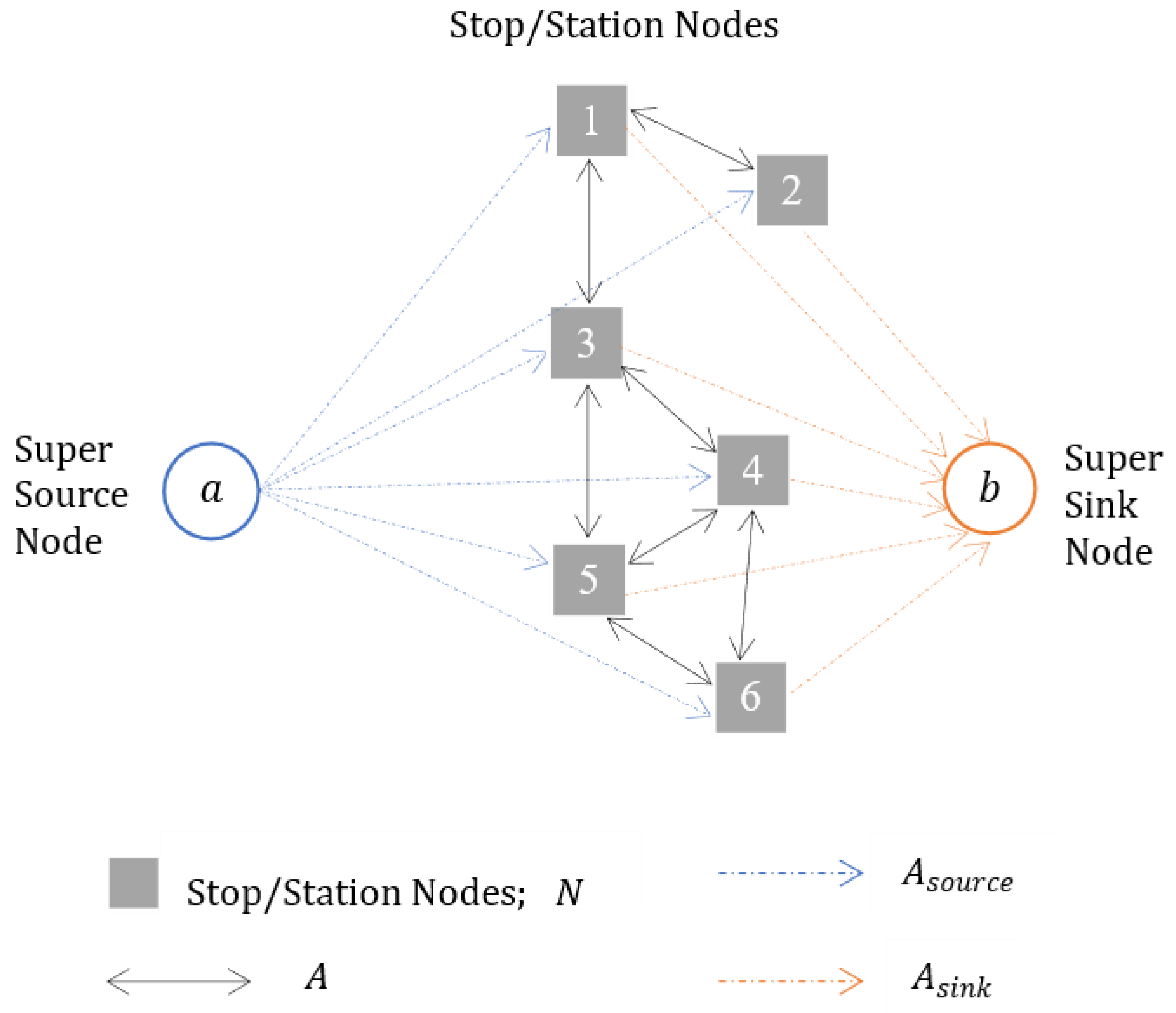
3.1. Problem Description

Consider a directed network $G=\left(N,A\right)$ with node set $N=\left\{1,\dots ,n\right\}$ representing stops and directed arc set $A$ representing the roads/links between stops. An arc ($i,j)$ between stops $i$ and $j$ exists only if $i$ and $j$ are adjacent and there is a direct road from $i$ and $j$. Without loss of generality, we assume that the roads between $i$ and $j$ are bidirectional. A subset $S\subseteq N$ ($D\subseteq N$) is distinguished as the set of supply/origin (demand/destination) nodes. A node $i\in S$ generates flows ${\omega }_{ij}>0$ for some $j\in D$, i.e., the number of passengers who would like to go from stop $i$ to stop $j$. ${\omega }_{ij}$ are represented in an Origin–Destination (OD) demand matrix and specified over a time period (e.g., hour, day, month). It is possible that a node $i$ is in both $S$ and $D$. For nodes $i$ and $j$ that are both in $S$ and $D$, it is not necessary that ${\omega }_{ij}={\omega }_{ji}$. For a supply node $k\in S$, the total outbound flow is ${\eta }_k={\displaystyle \sum }_{j\in D}{\omega }_{kj}$.

The passengers desire to go from their origins/boarding stops to their destinations on a single vehicle in the shortest possible time, which requires a route/line between each pair of stops in both directions. However, this is not practical from the perspective of the transit agency as it would be too costly. In this regard, the transit agency is to determine a route set $T$ to provide transport service to passengers. Each route $t\in T$ is a simple path with no repetition of nodes and composed of a starting node (terminal), an ending node (terminal), a set of intermediate nodes, and a set of arcs $\left(i,j\right)\in A$ connecting the nodes in $t$. On each route $t$, several vehicles with a specific capacity (${\beta }_t$) operate bidirectionally depending on the frequency (i.e., the number of vehicles per time unit) needed to satisfy the demand.

Passengers departing from $i$ and destined to $j$ may go directly on a single vehicle if a route passing through $i$ and $j$ exists. Otherwise, passengers may go indirectly to their destination by changing their route(s) at transfer points where two or more routes coincide. Even if it is possible to move from $i$ to $j$ using a single route, passengers may prefer to transfer depending on waiting times at the boarding and transfer points, which are imposed by the frequencies of the routes. Because making transfers is annoying for passengers, a transfer discomfort penalty (in time units) is used to control the number of transfers. Thus, the total travel time for passengers to arrive at their destination from their origin is the sum of the (1) in-vehicle travel time, (2) waiting time at the boarding stop, (3) waiting time(s) at the transfer stop(s), and (4) total penalty time resulting from transfers. The lower this total travel time and the number of transfers, the better for passengers.

Let ${\theta }_{ij}$ be the travel time (cost) from stop $i$ to stop $j$, with ${\theta }_{ij}$ being represented in a symmetric OD cost matrix as in the literature, i.e., ${\theta }_{ij}={\theta }_{ji}$. Thus, in-vehicle travel time is the sum of ${\theta }_{ij}$ for all $\left(i,j\right)$ on which passengers travel. Waiting times at boarding and transfer stops are not known (i.e., variables) and are determined by the headway of a route. The headway $h_t$ is the reciprocal of the frequency $f_t$, i.e., $h_t=1/f_t$, and indicates the time between two consecutive vehicles on a route. For instance, if $f_t=10 \mathrm{vehicles} \mathrm{per} \mathrm{hour}$, then $h_t=\frac{1}{10} \mathrm{hours} \mathrm{per} \mathrm{vehicle},$ which is $6 \min$. Assuming that the arrivals of passengers at boarding and transfer stops are uniformly distributed, the waiting times of passengers for a route are set to half of the headway as an approximation as in Esfeh et al. [46].

The transit agency needs to design a system taking into account the perspective of passengers. Specifically, the transit agency should attempt to minimize the total travel time of passengers, including in-vehicle travel, waiting, and transfer times, and to maximize the number of direct-traveler passengers (i.e., minimize the number of transfers). However, considering only passengers’ perspectives may be too costly for the transit agency. In this regard, it should also try to minimize the costs, e.g., the costs of trips as well as the fixed and operational costs of operating a vehicle fleet. In doing so, the transit agency needs to make several decisions, e.g., the number of routes to operate, the size of the vehicle fleet, the number of stops on a route, and the percentage of direct travelers. Depending on how several objectives are prioritized, the resulting systems may significantly differ; hence, an analysis of different scenarios needs to be conducted to devise a system balancing both perspectives.

3.2. The Proposed Model

We propose a mathematical programming model, namely the Public Transportation Planning Model (PTPM), to solve TNDFSP. We define PTPM on an extended network $GT=\left(NT,AT\right)$ obtained by adding (1) two dummy nodes to $N$, namely, $a$ and $b$ that act as a super source node and a super sink node, respectively, and (2) two sets of directed arcs to $A$, namely, $A_{source}=\left\{\left(a,i\right):i\in N\right\}$ and $A_{sink}=\left\{\left(i,b\right):i\in N\right\}$. That is, $NT=N\cup \left\{a\right\}\cup \left\{b\right\}$ and $AT=A\cup A_{source}\cup A_{sink}.$ We assume that all nodes are numbered, with a and b having the smallest and largest numbers, respectively. Figure 1 gives a schematic representation of the extended network $GT=\left(NT,AT\right)$.

Figure 1. Representation of a transit network $GT=\left(NT,AT\right)$.

All constructed routes start at node $a$ and end at node $b$. The model constructs a route $t\in T$ from scratch by selecting an arc $\left(a,i\right)\in A_{source}$, an arc $\left(j,b\right)\in A_{sink}$, and a set of arcs from $A$ that forms a path from $i$ and $j$, where nodes $i$ and $j$ are the starting and ending terminals of the route $t$, respectively. Figure 2 depicts the construction of routes in the model. In the figure, there are two routes: a-4-3-1-2-b and a-1-3-5-6-b. Because a and b are dummy nodes, the routes on the real physical network are 4-3-1-2 and 1-3-5-6. A similar approach that uses dummy nodes for selecting terminal nodes for routes can be found in the work of [47].

Figure 2. Illustration of the route design in a transit network $GT$.

To construct routes, we define binary decision variables $d_{ijt}$. Since a route is bidirectional, we define $d_{ijt}$ for arcs $\left(i,j|i, j\in N \wedge i<j\right)$ to reduce the number of decision variables. If $d_{ijt}=1$, then nodes $i$ and $j$ are consecutive stops in route $t$ and passenger flow is allowed in both directions $\left(i,j\right)$ and $\left(j,i\right)$ on the route. For $d_{ait}=1$ and $d_{jbt}=1$, stops $i$ and $j$ are the starting and ending terminals of route $t$. Another variable set associated with route construction is $y_{it}$ that take on the value of 1 if $i\in N$ is a part of route $t$ and 0, otherwise. It is possible to impose additional requirements on the routes, e.g., the minimum (maximum) number of stops in a route and the maximum distance of a route. The decision variables $f_t$ and $h_t$ represent the frequency and headway of a route $t$, respectively.

In addition to the variables above, we define (1) $x_{ijkt}$ that represent the flow of passengers of origin $k\in S$ in arc $\left(i,j\right)$ (i.e., traveling from stop $i$ to stop $j$) on route $t$, (2) $r_{ijkt}$ that represent the number of passengers of origin $k\in S$ who transfer at node $i$ to route $t$ with the next stop being node $j$, and (3) $v_t$ that represent the numbers of vehicles required for route $t$.

Below we summarize the sets, parameters, and decision variables used in the model.

Sets and Indices:

$T$ set of routes (t ∈ T)

$N$ set of stops (i, j,k ∈ N)

$A$ set of arcs (i, j)

$S$ set of departure/supply stops (S ⊆ N)

$a$ super source node for routes

$b$ super sink node for routes

$A_{source}$ the set of directed arcs of the form (a, i), i ∈ N

$A_{sink}$ the set of directed arcs of the form (i, b), i ∈ N

$NT$ node set of extended network GT = (NT, AT) with NT = N ∪ {a} ∪ {b}

$AT$ arc set of extended network GT = (NT, AT) with AT = A ∪ Asource ∪ Asink

$D_k$ set of arrival (destination) nodes for passengers of origin k ∈ S

Parameters:

${\beta }_t$ capacity of a vehicle in route t ∈ T

${\eta }_k$ the number of passengers of origin k ∈ S

${\omega }_{ik}$ the number of passengers of origin k ∈ S with destination i ∈ N

${\theta }_{ij}$ travel time from stop i to stop j

$\pi$ transfer penalty (in time units)

$\lambda$ maximum number of stops allowed for a route

$\mu$ minimum number of stops allowed for a route

$\rho$ time period for which OD demand matrix is specified

$M$ a big number enough to allow passenger flow

$\epsilon$ values for vehicle fleet size

$\varphi$ upper limit of vehicle fleet size of the transit agency

$ϵ$ a small number (ϵ = 10 × 10−6)

Decision Variables:

$x_{ijkt}$ the flow of passengers of origin k who travel from i to j on route t

$d_{ijt}$ 1, if arc (i, j), i < j, is selected to be in route t; 0, otherwise

$y_{it}$ 1, if stop i is in route t; 0, otherwise

$r_{ijkt}$ the number of passengers of origin k who transfer at node i to route t with next stop being node j

$f_t$ frequency of route t (vehicle per time unit, e.g., hour, minute)

$h_t$ headway of the route t (i.e., time between two consecutive vehicles for route t)

$v_t$ vehicle fleet required for route t

Objective Function Terms:

$$in-vehicle travel time: z_1= {\displaystyle \sum }_{\left(i,j\right)\in A}{\displaystyle \sum }_{k\in S}{\displaystyle \sum }_{t\in T}\left({\theta }_{ij}{x}_{ijkt}\right)$$

(1)

$$transfer time penalty: z_2= {\displaystyle \sum }_{\left(i,j\right)\in A}{\displaystyle \sum }_{k\in S}{\displaystyle \sum }_{t\in T}\left(\pi r_{ijkt}\right)$$

(2)

$$waiting time at boarding: z_3= {\displaystyle \sum }_{\left(i,j\right)\in A}{\displaystyle \sum }_{k=i}{\displaystyle \sum }_{t\in T}\left((h_t/2)x_{ijkt}\right)$$

(3)

$$waiting time at transfer: z_4= {\displaystyle \sum }_{\left(i,j\right)\in A}{\displaystyle \sum }_{k\in S}{\displaystyle \sum }_{t\in T}\left((h_t/2)r_{ijkt}\right)$$

(4)

$$vehicle fleet size: z_5= 2{\displaystyle \sum }_{\begin{array}{c}\left(i,j\right)\in A;\\ i<j\end{array}}{\displaystyle \sum }_{k\in S}{\displaystyle \sum }_{t\in T}\left({\theta }_{ij}{f}_t{d}_{ijt}\right)$$

(5)

The objective function term (1) represents total in-vehicle travel time of passengers. (2) finds the total transfer time of passengers who transfer and is used to penalize passenger transfers assuming that each transfer will take a specific time, i.e., penalty time. (3) and (4) compute waiting times of passengers at boarding and transfer stops, respectively. Objective function terms (1) through (4) represent the perspective of passengers. The objective function term (5) computes the total number of vehicles needed by the transit agency for all routes and is used as a proxy cost to denote the costs of the transit agency associated with operating the system. To explain how the fleet size is computed, suppose that the frequency of a route is $16 vehicles/hour$ and the route length in one direction is $15 \min$. Because the route is bidirectional and symmetric, the route length is $2\times 15 \min =30 \min$. Then, the number of vehicles needed on the route is $\left(16\frac{vehicles}{hour}\right)\times \left(0.5 h\right)=8 vehicles$.

Model PTPM: Public Transportation Planning Model (PTPM):

$\min Z_{passenger}= z_1+z_2+z_3+z_4$ $\min Z_{transitAgency}= z_5$		(6)
		(6′)
$s.t.$
${\displaystyle {\displaystyle \sum }_{i\in N}}{d}_{ait}=1$	$t\in T$	(7)
${\displaystyle {\displaystyle \sum }_{i\in N}}{d}_{ibt}=1$	$t\in T$	(8)
${\displaystyle {\displaystyle \sum }_{\begin{array}{c}j\in N;\\ i<j \wedge \left(i,j\right)\in A\end{array}}}{d}_{ijt}+{\displaystyle {\displaystyle \sum }_{\begin{array}{c}j\in N;\\ j<i \wedge \left(j,i\right)\in A\end{array}}}{d}_{jit}=2y_{it}$	$i\in N,t\in T$	(9)
${\displaystyle {\displaystyle \sum }_{i\in N}}{\displaystyle {\displaystyle \sum }_{\begin{array}{c}j\in N;\\ i<j \wedge \left(i,j\right)\in A \end{array}}}{d}_{ijt}\le \lambda -1$	$t\in T$	(10)
${\displaystyle {\displaystyle \sum }_{i\in N}}{\displaystyle {\displaystyle \sum }_{\begin{array}{c}j\in N;\\ i<j \wedge \left(i,j\right)\in A \end{array}}}{d}_{ijt}\ge \mu -1$	$t\in T$	(11)
${\displaystyle {\displaystyle \sum }_{i\in N}}{\displaystyle {\displaystyle \sum }_{\begin{array}{c}j\in N;\\ i<j \wedge \left(i,j\right)\in A\end{array}}}{d}_{ijt}\le \left|\overline{S}\right|-1$	$\overline{S}\subset N; 3\le \left|\overline{S}\right|\le \lambda -1$, $t\in T$	(12)
${\displaystyle {\displaystyle \sum }_{\begin{array}{c}j\in N;\\ \left(i,j\right)\in A\end{array}}}{\displaystyle {\displaystyle \sum }_{t\in T}}{x}_{ijkt}-{\displaystyle {\displaystyle \sum }_{\begin{array}{c}j\in N;\\ \left(j,i\right)\in A\end{array}}}{\displaystyle {\displaystyle \sum }_{t\in T}}{x}_{jikt}=\left\{\begin{array}{c}{\eta }_k, if i=k\\ -{\omega }_{ki}, if i\in D_k\\ 0, o.w\end{array}\right.$	$i\in N,k\in S$	(13)
${\displaystyle {\displaystyle \sum }_{k\in S}}\left(x_{ijkt}+x_{jikt}\right)\le M{d}_{ijt}$	$i,j\in N;i<j \wedge \left(i,j\right)\in A$ $t\in T$	(14)
$\left({\displaystyle {\displaystyle \sum }_{k\in S}}{x}_{ijkt}\right)/\rho \le {\beta }_t{f}_t$	$i,j\in N;\left(i,j\right)\in A$ $t\in T$	(15)
$x_{ijkt}={\displaystyle {\displaystyle \sum }_{\begin{array}{c}g\in N;\\ g\ne j \wedge \left(g,i\right)\in A\end{array}}}{x}_{gikt}+r_{ijkt}$	$i,j\in N; \left(i,j\right)\in A$ $k\in S; i\ne k$ $t\in T$	(16)
$2{\displaystyle {\displaystyle \sum }_{\begin{array}{c}\left(i,j\right)\in A;\\ i<j\end{array}}}{\displaystyle {\displaystyle \sum }_{k\in S}}{\displaystyle {\displaystyle \sum }_{t\in T}}\left({\theta }_{ij}{f}_t{d}_{ijt}\right)\le v_t$	$t\in T$	(17)
$f_t{h}_t=1$	$t\in T$	(18)
$r_{ijkt}\ge 0, x_{ijkt}\ge 0$	$i,j\in N; \left(i,j\right)\in A$ $k\in S,t\in T$	(19)
$f_t\ge 0, h_t\ge 0+ϵ$	$t\in T$	(20)
$v_t\ge 0, Integer$	$t\in T$	(21)
$d_{ijt}\in \left\{0,1\right\}$	$\left(i,j\right)\in AT$ $t\in T$	(22)
$y_{it}\in \left\{0,1\right\}$	$i\in N, t\in T$	(23)

PTPM minimizes the costs of passengers (6) and the transit agency (6′); hence, it is a multi-objective optimization problem. The objective function (6) minimizes the total travel time of all passengers and (6′) minimizes the transit agency’s cost, which is represented as the fleet size required to operate the system. Constraints (7) requires each route $t$ to have an arc from the super source node $a$ to a stop $i\in N$, which becomes the starting terminal of that route. Constraints (8) require each route $t$ to have an arc from a stop $i\in N$ to the super sink node $b$, with $i$ being the ending terminal of that route. If the starting and ending terminals are known in advance, they can be specified using (7) and (8). Constraints (9) ensure that each stop in a route is connected to two other nodes (stops or super nodes) as shown in Figure 2.

Constraints (10) and (11) impose upper and lower limits on the number of stops in a route, respectively. Constraints (12) eliminate subtours in the routes using the Dantzig–Fulkerson–Johnson (DFJ) subtour elimination formulation [48], where $\overline{S}$ is a subset of stops with the specified cardinality. The number of such constraints increases exponentially with the cardinality of the node set $\left|N\right|$ and hence, they cannot be used directly unless $\left|N\right|$ is very small. Therefore, we add subtour elimination constraints (12) during the solution process as described in Algorithm 1 only when the candidate solutions violate them.

Constraints (13) are the flow conservation constraints of passengers at the stops and ensures that passengers move from their origins to their destinations through some routes. Constraints (14) couple passenger flow variables and arc selection variables and allow passenger flows only when an arc is selected to be in a route.

Constraints (15) ensure that a frequency for each route $t$, $f_t$, is determined considering the maximum passenger load on the route, which is equivalent to the maximum value on the left-hand side of (15). In other words, $f_t$ can be considered as the number of vehicles needed per time unit to satisfy the demand for route $t$. Constraints (16) are the flow balance constraints for the transfer of passengers. They state that the number of passengers of origin $k$ on arc $\left(i,j\right)$ in route $t$ is equivalent to the number of passengers already traveling on route $t$ and the number of passengers that transfer to route $t$ at node $i$ and move to $j$.

Constraints (17) compute the number of vehicles for each route. Because routes serve in two directions, there is a multiplier of $2$ on the left-hand side. Constraints (17) with constraints (15) ensure that vehicles are not overcrowded because each route has a sufficient number of vehicles to carry passengers. Constraints (18) state that the headway of a route is the inverse of the frequency of that route. Finally, Constraints (19)–(23) define the variables. Passenger flow and transfer variables, as well as headway variables, are defined to be non-negative. Because the problem is strategic, fractional values regarding passenger flow and transfers may be accepted. To avoid an undefined frequency evaluation due to constraint set (18), we set a lower bound with a small number, $ϵ$, for the headway variable in constraint (20).

The resulting PTPM is a nonlinear mixed integer programming model because constraints (17) and (18) and objective function terms (3), (4), and (5) consist of multiplications of decision variables.

4. Solution Methodology

4.1. Multi-Objective Optimization

PTPM is a multi-objective optimization model. In order to solve it using off-the-shelf software and obtain Pareto-optimal solutions, we convert it into a single-objective optimization model using the $\epsilon$-Constraint method. We move the transit agency’s objective function (6′) to the constraint set as in (24) where the left-hand side represents the vehicle fleet size and the right-hand side represents an alternative level for vehicle fleet size. We solve the resulting single-objective optimization model for different levels of the vehicle fleet size $\epsilon$ to find Pareto-optimal solutions.

${\displaystyle {\displaystyle \sum }_{t\in T}}{v}_t\le \epsilon$

$\epsilon \le \varphi$

(24)

It is worth mentioning that by restructuring the PTPM to include an objective function that exclusively focuses on minimizing the number of vehicles, a lower bound for the vehicle fleet size can be determined. The resultant solution derived from this transformation serves as a reliable reference point for determining the minimum requirement of the vehicle fleet.

4.2. Subtour Elimination

The number of subtour elimination constraints (12) increases exponentially with the cardinality of the node set $\left|N\right|$ and hence, they cannot be used directly while solving PTPM unless $\left|N\right|$ is very small. For this reason, we add constraints (12) during the solution process only when candidate solutions violate them. The basic idea is to solve PTPM without constraints (12) and add only those constraints of (12) that eliminate subtours, i.e., the cuts, whenever there is an integer solution with subtours.

When PTPM is solved without constraint (12), subtours may occur in a route $t\in T$. For each integer solution for a route set $T$, we can check and quickly identify subtours and add specific cut (12) to separate them. We run this intervention procedure within a Lazy Constraints Callback function of Gurobi. Lazy Constraints are constructed when the user defines a violation for an integer solution. Algorithm 1 summarizes the steps of the intervention procedure.

Algorithm 1: Subtour Elimination.

Step 0: Start solving PTPM without constraints (12) using Gurobi. Due to the formulation consisting of integer decision space, the solver unfolds a branch and bound tree. Step 1: When the solver finds an integer solution in any node of the branch and bound tree, run the Lazy Constraints Callback function defined for detecting subtours. Step 2: If the callback function finds subtour(s) in the integer solution, go to step 3. Otherwise, go to step 4. Step 3: Add corresponding subtour elimination constraint (12) for violating the integer solution. Step 4: Continue exploring the branch and bound tree nodes.

4.3. Solving Large-Size Instances

We can obtain good solutions for small instances such as the Mandl dataset in minutes (see Section 5) with Gurobi. However, Gurobi cannot find feasible integer solutions for large-size instances such as a real-world application defined in Section 6. In this regard, we develop a solution methodology for large-size instances based on essentially providing the solver with a good warm-start solution for route design variables, $d_{ijt}$. We obtain warm-start solutions by exploiting the Node Relaxation Heuristic (NoRelHeur) utility of Gurobi and solving relaxed versions of PTPM. NoRelHeur is an embedded heuristic algorithm of Gurobi and can be used when the root node relaxation consumes too much time during the Branch&Cut (B&C) solution procedure. In applying Gurobi with NoRelHeur, NoRelHeur first tries to find a high-quality feasible solution in the allocated time and then Gurobi implements the branch and cut algorithm with the warm-start feasible solution found by NoRelHeur. The solution procedure is summarized in Algorithm 2.

In the application of Algorithm 2, we solve a relaxed, single-objective version of PTPM, PTPM_Rel, obtained by eliminating constraints (17), (18), (20), and (21), as well as terms (3) and (4) in the objective function (6). The eliminated constraints and objective function terms are related to the vehicle fleet size, as well as to the frequency and headway decisions. PTPM_Rel tries to minimize the sum of in-vehicle travel time and transfer penalty time, i.e., $z_1+z_2$, with constraints (7)–(16), (19), (22), and (23) ignoring the objective function (6′). While solving PTPM_Rel, we apply Algorithm 1 as necessary to eliminate subtours.

To obtain a warm-start solution for $d_{ijt}$ to use in solving PTPM, we solve PTPM_Rel in two phases. In the first phase, we solve PTPM_Rel only for a specific $k\in S$, i.e., PTPM_Rel_k. This allows a route network to be constructed considering only passengers of origin $k$. To ensure that the route set is connected and consists of all stops, there should be demand for passengers of origin $k$ at all other nodes, i.e., $k$ should be selected such that ${\omega }_{kj}>0, \forall j\in N$. If such a $k$ does not exist, we select a $k$ with the highest $\left|D_k\right|$ and assign an arbitrary positive value as a demand for $j\ne k \mathrm{with} {\omega }_{kj}=0$. Let $d_{ijt}^{Rel\_k}$ represent the values of decision variables $d_{ijt}$ obtained after solving PTPM_Rel_k. In the second phase, we solve PTPM_Rel with the original OD demand matrix using $d_{ijt}^{Rel\_k}$ as an initial solution for $d_{ijt}$. Let $d_{ijt}^{Rel}$ represent the values of decision variables $d_{ijt}$ obtained after solving PTPM_Rel. In the final step of Algorithm 2, we solve PTPM with the original OD matrix for different vehicle fleet levels using $d_{ijt}^{Rel}$ as the warm-start solution. We use Gurobi with NoRelHeur in solving PTPM_Rel_k and PTPM_Rel while we use Gurobi in solving PTPM.

Algorithm 2: Solution Procedure for Large Instances.

Input: A transit network instance with OD demand and distance matrices. Step 1: Obtain a route network considering passengers of a specific origin $k$. Solve PTPM_Rel_k for a specific $\mathrm{k}$ using Gurobi with NoRelHeur. Save ${\mathrm{d}}_{\mathrm{ijt}}^{\mathrm{Rel}\_\mathrm{k}}$ that represent the values of decision variables for ${\mathrm{d}}_{\mathrm{ijt}}$ in the solution of PTPM_Rel_k. Step 2: Obtain a route network considering the original OD demand matrix. Solve PTPM_Rel setting ${\mathrm{d}}_{\mathrm{ijt}}^{\mathrm{Rel}\_\mathrm{k}}$ as an initial solution using Gurobi with NoRelHeur Save ${\mathrm{d}}_{\mathrm{ijt}}^{\mathrm{Rel}}$ that represent the values of decision variables for ${\mathrm{d}}_{\mathrm{ijt}}$ in the solution of PTPM_Rel. Step 3: Obtain feasible integer solutions for TNDFSP Solve PTPM setting ${\mathrm{d}}_{\mathrm{ijt}}^{\mathrm{Rel}}$ as an initial solution and using Gurobi for different vehicle fleet sizes to obtain Pareto-optimal solutions. Output: Pareto optimal solutions for the transit network for varying vehicle fleet sizes.

5. Computational Tests Using Benchmark Instances

In this section, our goal is to show that PTPM works correctly and produces better results than the exact and heuristic methods proposed in the literature. We conduct two sets of experiments. In the first set of experiments, we ignore waiting times at boarding and transfer points because the studies with which we compare our results use different assumptions in modeling waiting times and hence, the results are not comparable when waiting times are taken into account. In the second set of experiments, we obtain solutions considering waiting times.

To verify and validate PTPM, we use Mandl benchmark instances for which features are given in Table 2. We do not use Mumford instances because they are considered inappropriate for TNDFSP tests due to highly unrealistic frequencies [9]. We conduct experiments with Gurobi 9.5 solver using the Julia programming language [49] and JuMP modeling language package [50] on a computer of an Intel Core i7@3.30 GHz with 16 GB of RAM. We use the default settings of Gurobi parameters except for NonConvex = 2, MIPFocus = 1, and BranchDir = 1. NonConvex = 2 tells Gurobi that the model is nonlinear. MIPFocus = 1 emphasizes improving the primal bound. BranchDir = 1 requires the up-branch to be explored first when a branching decision is to be made. This setting reduces the number of explored nodes and decreases the computer’s RAM load especially for large-size instances. The runtime for all experiments on Mandl instances is 3600 s. Vehicle capacity is 50 with a load factor of $1.25$, i.e., $40\times 1.25=50$.

Table 2. Features of benchmark instances.

Network	Number of Nodes/Edges	Number of Routes	Node Limits Min/Max	Transfer Penalty (Mins.)	Number of Non-Zero OD Demand Pairs	Total Passenger Demand	Demand Period (Mins.)	Vehicle Capacity
Mandl	15/21	4, 6, 8, 10, 12	2/8	5	172	15,570	60	50

Pareto-optimal solutions are generated with respect to different levels of vehicle fleet size. We start by setting a vehicle fleet size less than or equal to an upper bound of the vehicle fleet and then gradually reduce it step by step. This approach is considered safe because if the number of vehicles is infeasible, the model itself results in infeasibility.

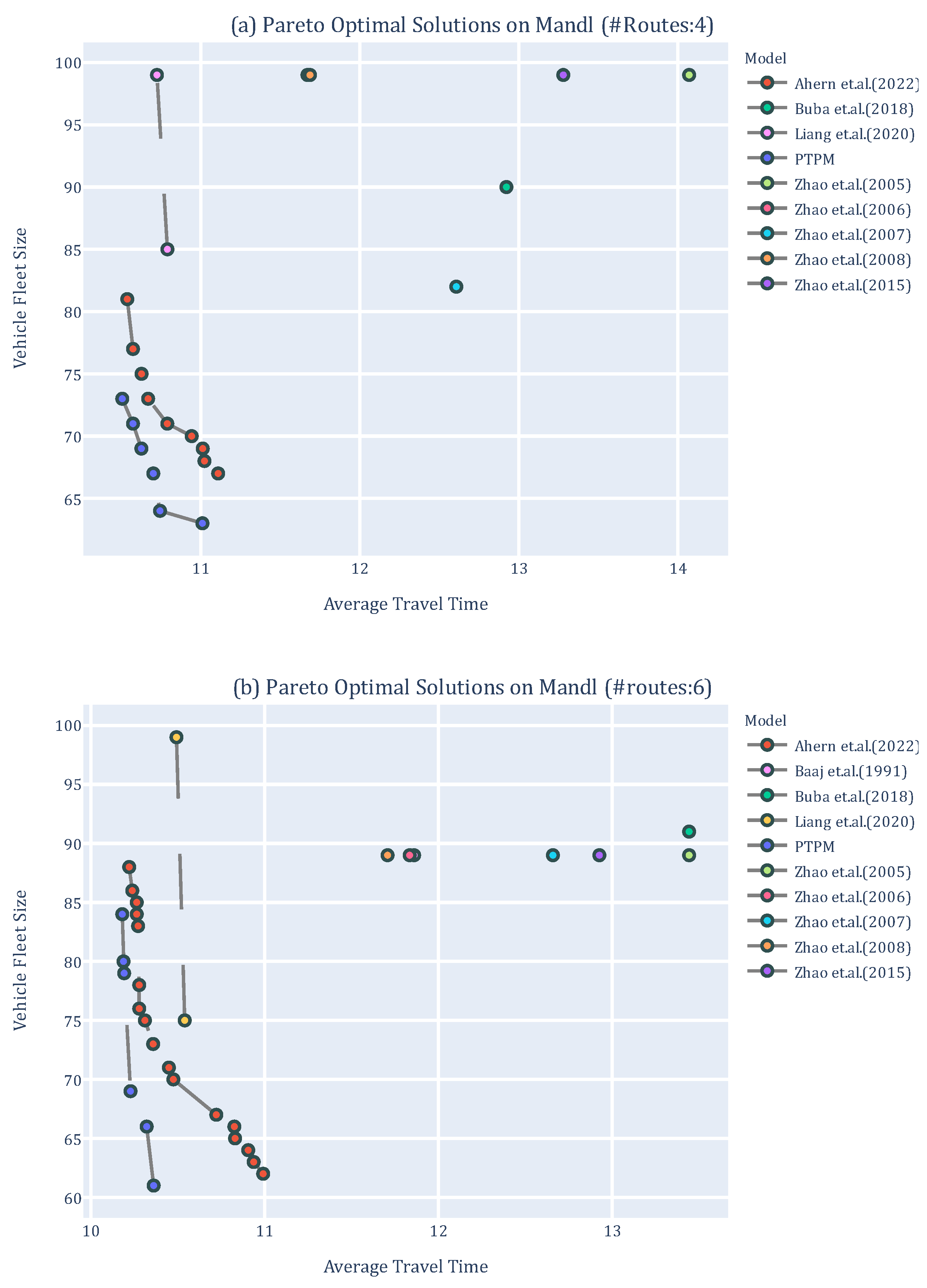
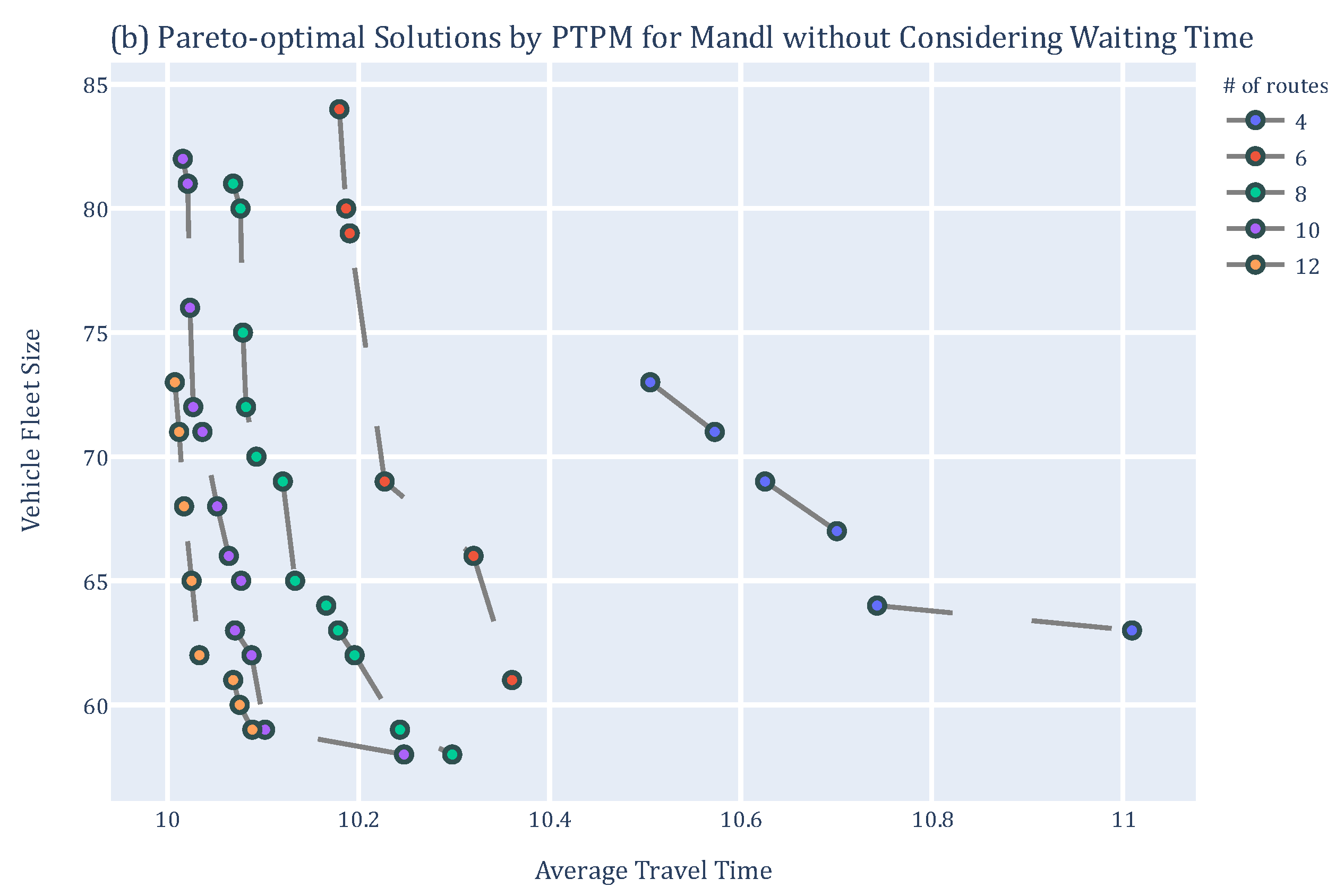
5.1. Benchmark Tests without Considering Waiting Times

In the literature, few studies model waiting times at boarding and transfer nodes and solve benchmark instances. However, the rules of passenger assignment in these studies differ from our system optimal approach, which results in different waiting times in different studies. For example, Ahern et al. [36] use the frequency share method while Liang et al. [37] assign passengers to routes based on the directness of the trip and the number of transfers. In this regard, the results of different studies are not comparable when waiting times are considered. Therefore, we compare our results with those proposed in the previous studies without considering waiting times, i.e., we solve PTPM with $Z_{passenger}=z_1+z_2$ by varying vehicle fleet size to obtain Pareto-optimal solutions as described before.

We present the results in the objective space with the x-axis representing the average travel time consisting of in-vehicle travel time and transfer penalty time and the y-axis representing the vehicle fleet size. Figure 3 indicates the results of PTPM, as well as the results of the studies of Ahern et al. (2022) [36], Bagloee and Ceder (2011) [40], Baaj and Mahmassani (1991) [12], Buba and Lee (2018) [38], Liang et al. (2020) [37], Zhao et al. (2005) [42], Zhao and Zeng (2006, 2007, 2008) [43,44,45], and Zhao et al. (2015) [41] for different numbers of routes. We show only the results reported in the related studies. We remark that all studies with which we compare our results are (meta)heuristic-based because there does not exist mathematical programming-based studies that attempt to solve benchmark instances with the objective of minimizing the travel time.

Figure 3. Pareto-optimal solutions generated by PTPM and different studies in the literature without considering waiting times [12,36,37,38,40,41,42,43,44,45].

The results indicate that PTPM can provide better Pareto-optimal solutions than other algorithms. The study closest to ours in performance is Ahern et al. [36]. As the fleet size increases, the results of PTPM and Ahern et al. [36] get closer. However, as the fleet size decreases, i.e., when the problems are harder to solve, PTPM produces much better results.

The details of the computational results including the stops, vehicle fleet size, headways and frequencies of routes, average passenger cost and percent of transfers can be accessed through the following repository (File S1, Supplementary Materials).

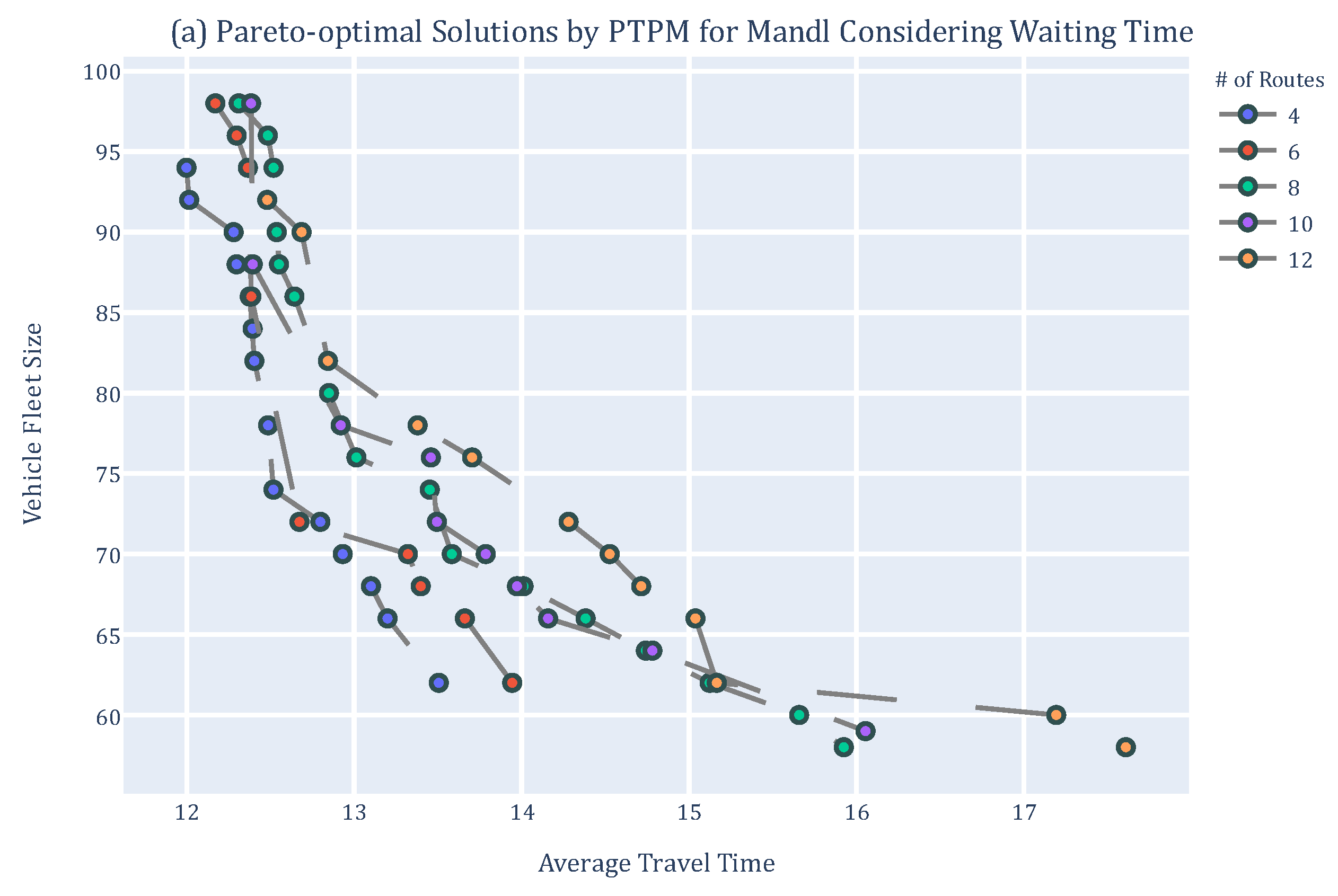
5.2. Tests including Waiting Times

Figure 4a,b present Pareto-optimal solutions generated by PTPM for Mandl instances considering waiting times and without considering waiting times, respectively. The results in Figure 4a indicate that, for a fixed fleet size, the average travel time decreases as the number of routes decreases because more vehicles can be assigned to routes, which enables waiting times at boarding and transfer stops to be decreased. However, as the number of routes decreases, the passenger load gets higher causing more discomfort to passengers. In this regard, there is a need to establish a balance between passenger discomfort resulting from a high passenger load and passenger discomfort resulting from long travel times. The results in Figure 4b indicate that, for a fixed fleet size, the average travel time increases as the number of routes decreases contrary to the results in Figure 4a. As the number of routes decreases, the number of direct travelers increases, and hence, the average in-vehicle travel time increases. The results emphasize the importance of incorporating waiting times at boarding and transfer points as the results without waiting times may mislead the transit agency in developing plans.

Figure 4. Pareto-optimal solutions generated by PTPM for Mandl instances considering waiting times.

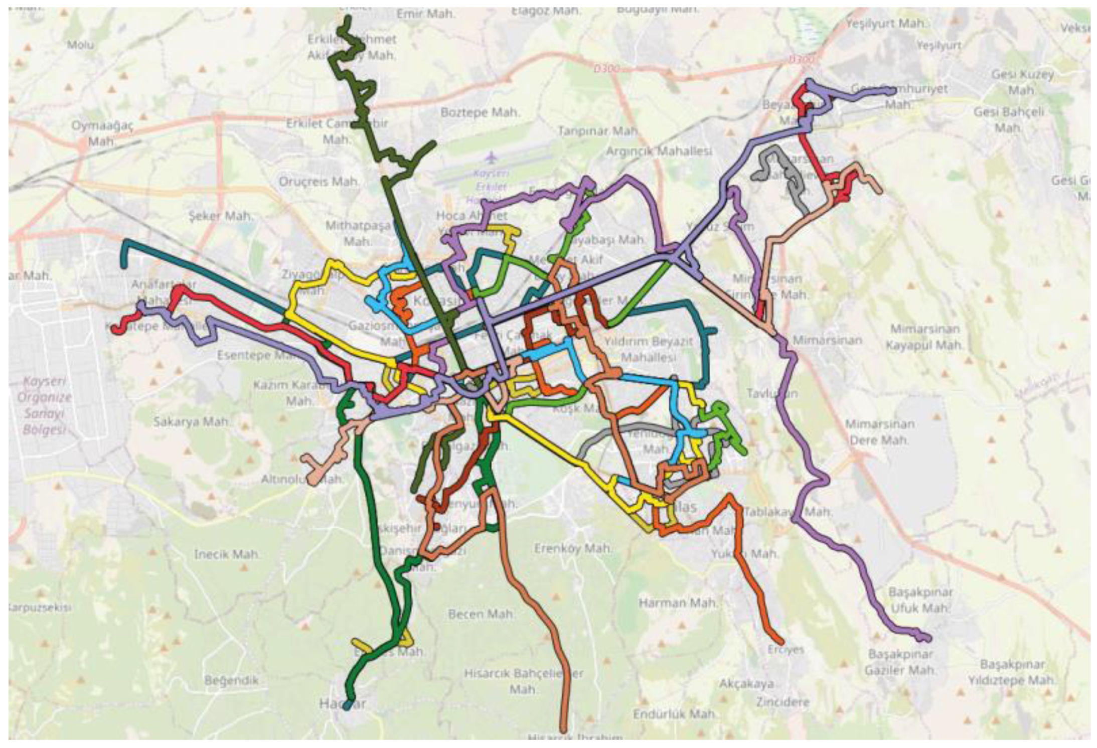
6. A Real-World Application

In this section, we present the results of computational tests conducted for instances defined on a real bus transit network in the city of Kayseri, located in the Central Anatolian Region in Türkiye. Kayseri has a population of about 1.5 million. The current public transport system consists of a tram network and a bus transit network. The tram and bus networks intersect at certain points; however, the tram network passes through a limited number of streets and has limited capacity. The bus network is currently the main public transport system. The number of stops in both directions in the current bus transit system is over 3000, which is pretty high for the size of a city such as Kayseri. In this regard, designing a trunk-and-feeder system is considered as an alternative. Our goal in this study is to determine trunk lines/routes on the stops selected by Kayseri Transportation Inc. considering the demand intensity and location diversity. The Kayseri204 network consists of 204 nodes and 405 edges. The features of the instances considered are given in Table 3.

Table 3. Features for Kayseri204 transit network instances.

Network	Number of Nodes/Edges	Number of Routes	Node Limits (Min/Max)	Transfer Penalty (Mins.)	Number of Non-Zero OD Demand Pairs	Total Passenger Demand	Demand Period (Mins.)	Vehicle Capacity
Kayseri204	204/405	15, 20, 25	2/25	15	13,338	205,090	1000	50

We conduct tests with Gurobi 9.5 solver on an Intel(R) Xeon(R) Gold 6150@2.70 GHz computer with 256 GB of RAM with the parameter settings of Gurobi defined earlier. Since Kayseri204 is a large network, we run Algorithm 2 to find solutions for the instances. In the application of Algorithm 2, we set run times as follows: Step 1: NoRelHeurTime = 2000, TimeLimit = 3000; Step 2: NoRelHeurTime = 50,000, TimeLimit = 60,000; and Step 3: TimeLimit = 23,400, i.e., the total runtime of Algorithm 2 is 86,400 s. We remark that we provide the solution obtained in Steps 1 and 2 as a warm-start solution in Step 3, where we run just the B&C algorithm of Gurobi.

We obtain results for 15-, 20-, and 25-route options by setting the number of vehicles to 150, 160, 180, 200, 220, 250, and 300. We assume a transfer penalty of 15 min as in Arbex and da Cunha [39] and Borndörfer and Karbstein [51].

OD demand and distance matrices as well as the features of Pareto-optimal solutions, including the average travel time, vehicle fleet size, and optimality gap, can be accessed through the following repository (File S2, Supplementary Materials).

6.1. Travel Time vs. Number of Vehicles

Figure 5 gives Pareto-optimal solutions for different numbers of routes. The results indicate that the 15-route solution dominates 20- and 25-route solutions with respect to the average travel time per passenger and vehicle fleet size. Similar to Mandl cases, for a fixed vehicle fleet size, average travel time for 15-route solution is better than 20-route and 25-route solutions. This is because more vehicles can be assigned to the routes in the 15-route instance, which decreases waiting times at boarding and transfer points. When the required number of routes increases, more vehicles may be needed to ensure a certain service level.

Figure 5. Pareto-optimal solutions for Kayseri204 instances.

We remark that feasible solutions cannot be obtained for the vehicle fleet sizes lower than 150, 160, and 180 for the 15-route, 20-route, and 25-route instances, respectively. A sample solution for 15 routes and 150 vehicles is presented in Figure 6 on the Kayseri map, where each color corresponds to a different route. Parts of some routes coincide and hence overlap in some segments.

Figure 6. Sample solution for 15 routes and 150 vehicles for the Kayseri204 network.

Table 4 details the results with respect to the average in-vehicle travel time (AIVT), waiting time (AWT), transfer penalty time (ATP), optimality gap (Gap%), average travel time (ATT), and headway (AH) for different numbers of routes. The table shows how average in-vehicle travel times, waiting times, and transfer penalty times change with the increasing number of routes and vehicle fleet sizes. For a fixed number of routes, as the fleet size increases, all related times essentially get better. As the number of routes increases, average transfer penalty times decrease because the number of direct travelers increases. On the other hand, average waiting times increase because average headways increase as fewer vehicles can be assigned to the routes. Because average in-vehicle travel times are close to each other and the improvements in the transfer penalty time are lower than the deterioration in waiting times, the average waiting time becomes dominant and generally causes the total average travel time to increase for a fixed fleet size. That is, for a fixed fleet size, increasing the number of routes does not improve the service level with respect to total average travel time.

Table 4. Average travel times for Kayseri204 network instances.

Route	Fleet	AIVT	AWT	ATP	ATT	AH	Gap (%)
15	150	26.69	13.74	8.51	48.94	21.67	57.82
	160	26.31	12.22	7.83	46.35	19.56	55.47
	180	26.07	10.31	7.04	43.43	16.9	52.47
	200	25.87	9.13	6.89	41.89	14.93	50.73
	220	25.96	8.06	6.72	40.75	12.68	49.34
	250	25.84	7.29	6.76	39.89	12.02	48.25
	270	25.68	6.59	6.82	39.10	10.48	47.20
	300	25.69	6.02	6.83	38.54	9.62	46.44
20	160	27.53	17.68	8.48	53.69	39.3	61.56
	180	26.70	14.68	6.46	47.84	31.2	56.85
	200	26.21	12.22	6.01	44.44	26.8	53.55
	220	25.93	10.93	6.00	42.86	22.33	51.83
	250	25.61	9.42	5.87	40.90	20.31	49.53
	270	25.39	8.67	6.00	40.06	18.38	48.47
	300	25.36	7.79	5.91	39.06	15.51	47.15
25	180	26.12	15.83	5.87	47.82	44.27	56.83
	200	26.11	14.48	6.20	46.80	36.39	55.89
	220	25.55	12.96	5.96	44.47	32.21	53.58
	250	25.52	10.72	5.16	41.40	25.17	50.14
	270	25.36	9.91	5.12	40.39	22.47	48.90
	300	25.33	9.32	5.19	39.85	22.05	48.20

AIVT: average in-vehicle time, AWT: average waiting time, ATP: average transfer penalty, ATT: average travel time (AIVT + AWT + ATP), AH: average headway. These units are in minutes.

Table 4 indicates that optimality gaps change from 47.15% to 61.56%. The resulting high gaps occur because Gurobi cannot improve the linear programming relaxation bounds, i.e., the solutions found by Gurobi may actually be much better. To check the quality of solutions found by Algorithm 2, we have solved Mandl benchmark instances using Algorithm 2 as well. The results indicate that Algorithm 2 produces solutions that are very close to and sometimes better than those found by Gurobi without NoRel with optimality gaps of about 25% on average. Considering the fact that the solutions found by the proposed model using Gurobi with these high optimality gaps are better than solutions found by the state-of-the-art algorithms, we think that the solutions obtained for the Kayseri204 network may be much better.

We remark that even though the gaps are high, this study is the first to obtain solutions for instances significantly larger than those in the literature using mathematical programming and off-the-shelf software (204 nodes and 13,338 OD pairs in comparison to 84 nodes and 363 OD pairs in the literature).

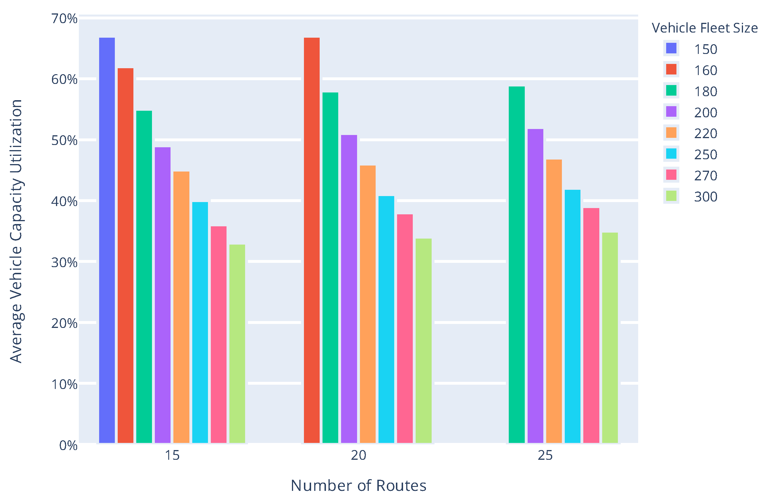
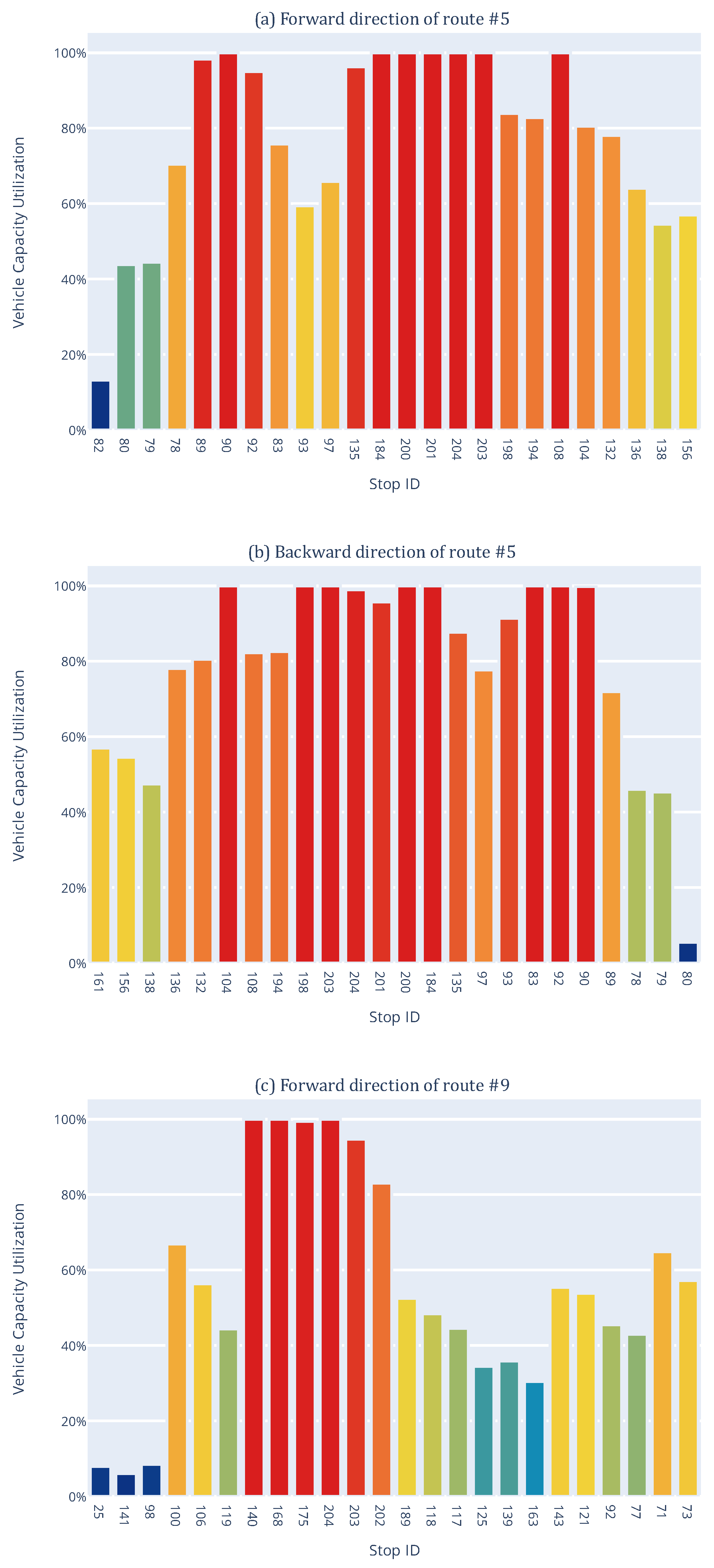
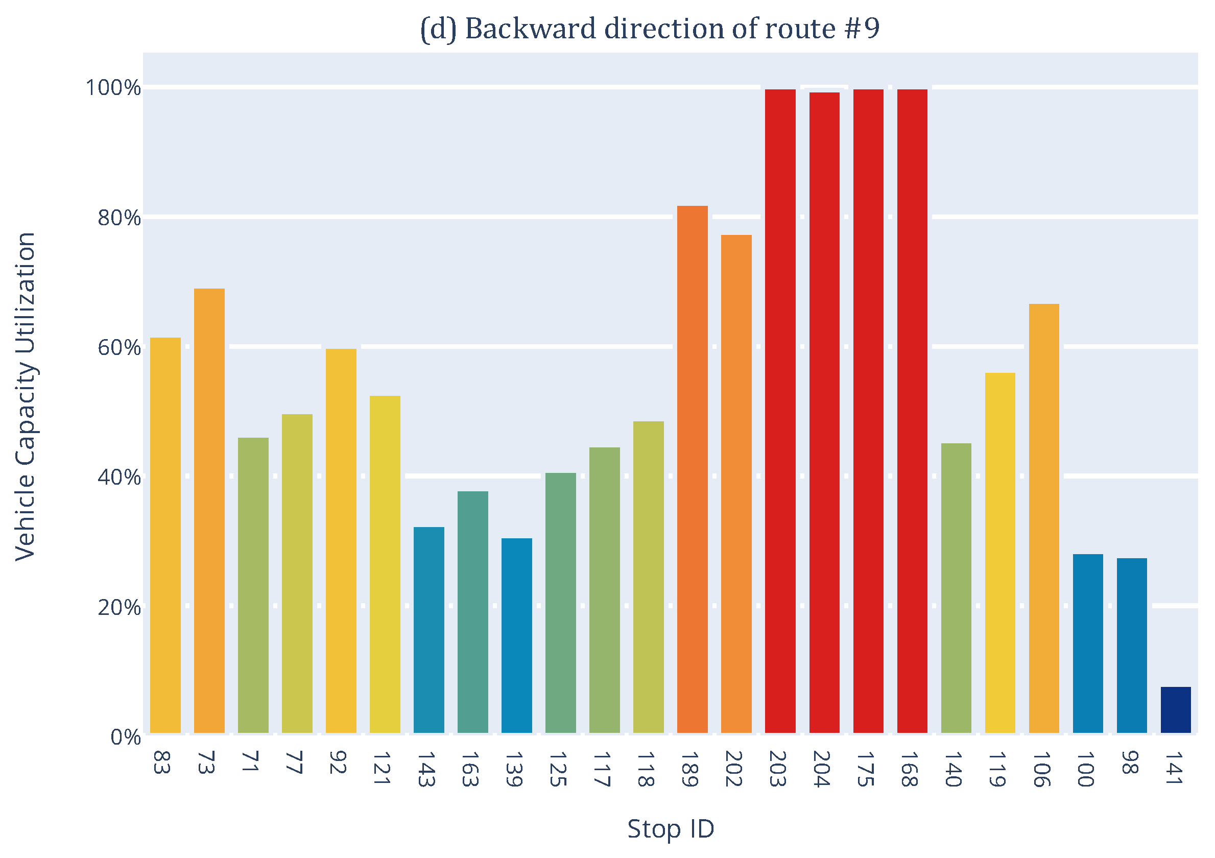
6.2. Utilization of Vehicle Capacity

Analyzing the utilization of vehicle capacity for a route helps the transit agency to evaluate route crowding and under-utilization issues. The utilization of vehicle capacity for a route set can be computed as follows: Let $n{v}_t$ represent the number of vehicles assigned to route $t$, $vc$ the capacity of a vehicle, $p{l}_{ijt}$ passenger load on the link from $i$ to $j$ on route $t$, and $n{l}_t$ the number of links on route $t$. The utilization of vehicle capacity for the link from $i to j$ on route $t$ is $vc{u}_{ijt}=\frac{p{l}_{ijt}}{vc\times n{v}_t}\times 100$, the average utilization of vehicle capacity for route $t$ is $ac{u}_t=\frac{{{\displaystyle \sum }}_{ij}p{l}_{ijt}}{n{l}_t}$, and the average utilization of vehicle capacity for the whole route set is $u=\frac{{{\displaystyle \sum }}_t(ac{u}_t\times n{v}_t)}{{{\displaystyle \sum }}_t n{v}_t}$.

Figure 7 gives the average utilization of vehicle capacity for different numbers of routes and vehicle fleet sizes for the Kayseri204 network. For a fixed number of routes, the average utilization of vehicle capacity decreases as the vehicle fleet size increases.

Figure 7. Average utilization of vehicle capacity for Kayseri204 instances.

Figure 8 depicts an example analysis of the most and least utilized routes for a 15-route instance with 150 vehicles. Figure 8a–d show the utilization of vehicle capacity on the links of the busiest route (the least busy route), route #5 (route #9), in forward and backward directions, respectively. A bar in the figure indicates the utilization of vehicle capacity for the link between two consecutive nodes in the x-axis. For instance, the first blue bar in Figure 8a represents the utilization of vehicle capacity for the link from 82 to 80. The results indicate that the intensity of passengers and hence the utilization level gets higher towards the middle segment of the routes as expected, reaching 100% for some links. Even though route #9 is the least busy route, the utilization level for some links is 100%.

Figure 8. Utilization of vehicle capacity for the busiest and the least busy routes for a 15-route solution with 150 vehicles.

7. Conclusions and Future Research Direction

In this paper, we address the transit network design and frequency setting problem (TNDFSP) that aims at designing the routes and determining the frequencies of the routes to satisfy passenger demand in a transit network. We propose a novel mathematical programming model for TNDSFP that incorporates the features of real-life transit network systems. The proposed model reflects the views of both passengers and the transit agency by considering in-vehicle travel time, transfers, waiting times at the boarding and transfer stops, overcrowding and under-utilization of vehicles, and vehicle fleet size. The model is the first to determine routes and their frequencies simultaneously from scratch, i.e., without using line and frequency pools while considering the aforementioned issues such as transfers and waiting.

We solve the proposed model using Gurobi. We conduct computational tests using Mandl benchmark instances and a real-world transit network. The first group of tests indicates that the proposed model works correctly and produces better Pareto-optimal solutions than those obtained by the state-of-the-art algorithms. The second group of tests shows how what-if analyses may be helpful in designing a transit network system. The main insights from what-if analyses may be summarized as follows:

• For a fixed fleet size, the total average travel time gets better with a decreasing number of routes because more vehicles can be assigned to the routes.
• For a fixed fleet size, average waiting times at boarding and transfer points increase with the increasing number of routes because fewer vehicles can be assigned to the routes.
• For a fixed fleet size, the average transfer penalty time decreases because the number of direct travelers increases with the increasing number of routes.
• For a fixed number of routes, the total average travel time, average transfer penalty time, and average waiting times improve with the increasing fleet size.
• The average utilization of vehicle capacity decreases with an increasing vehicle fleet size.
• The average utilization of vehicle capacity may reach up to 100% on some links even for the least busy routes.
• More vehicles may be needed to ensure a certain service level with respect to the total average time with the increasing number of routes.
• Incorporating waiting times and transfer times as well as the vehicle fleet size into the modeling may change the results significantly and hence is of high importance.

The insights imply that, instead of investing heavily in maintaining or expanding existing routes or lines, transit agencies might consider dramatically modifying the current lines or establishing entirely new ones. They should also be aware that passenger demand patterns will change over time, making even optimized route planning suboptimal in the long run.

We remark that the insights may change depending on the values of different parameters. However, the results indicate that the model can be useful as a decision aid for designing a transit network system or evaluating a current system.

This study is the first to obtain solutions for instances significantly larger than those in the literature using mathematical programming and off-the-shelf software (204 nodes and 13,338 OD pairs in comparison to 84 nodes and 363 OD pairs in the literature); however, the model is difficult to solve for large-scale problems in designing a system from scratch and hence, there is a need to improve the solvability of the model as a future research direction. In this regard, problem-specific cuts, decomposition algorithms, and heuristics may be developed and incorporated into the solution procedure. Moreover, methods to reduce the sizes of the problems, e.g., network analysis or aggregation rules, may be proposed.

References

1. United Nations Department of Economic and Social Affairs (UN DESA). 2018 Revision of World Urbanization Prospects. 2018. Available online: https://population.un.org/wup/Publications/Files/WUP2018-PressRelease.pdf (accessed on 9 September 2023).
2. Li, T.; Burke, M.; Dodson, J. Transport impacts of government employment decentralization in an Australian city—Testing scenarios using transport simulation. Socio-Econ. Plan. Sci. 2017, 58, 63–71. [Google Scholar] [CrossRef]
3. Ceder, A.; Wilson, N.H. Bus network design. Transp. Res. Part B Methodol. 1986, 20, 331–344. [Google Scholar] [CrossRef]
4. Laporte, G.; Mesa, J.; Ortega, F.; Perea, F. Planning rapid transit networks. Socio-Econ. Plan. Sci. 2011, 45, 95–104. [Google Scholar] [CrossRef]
5. Murray, A.T. Strategic analysis of public transport coverage. Socio-Econ. Plan. Sci. 2001, 35, 175–188. [Google Scholar] [CrossRef]
6. Carrese, S.; Gori, S. An Urban Bus Network Design Procedure. Transp. Plan. 2002, 64, 177–195. [Google Scholar] [CrossRef]
7. Schöbel, A. Line planning in public transportation: Models and methods. OR Spectr. 2011, 34, 491–510. [Google Scholar] [CrossRef]
8. Farahani, R.Z.; Miandoabchi, E.; Szeto, W.; Rashidi, H. A review of urban transportation network design problems. Eur. J. Oper. Res. 2013, 229, 281–302. [Google Scholar] [CrossRef]
9. Durán-Micco, J.; Vansteenwegen, P. A survey on the transit network design and frequency setting problem. Public Transp. 2021, 14, 155–190. [Google Scholar] [CrossRef]
10. Zhou, Y.; Yang, H.; Wang, Y.; Yan, X. Integrated line configuration and frequency determination with passenger path assignment in urban rail transit networks. Transp. Res. Part B Methodol. 2021, 145, 134–151. [Google Scholar] [CrossRef]
11. Bourbonnais, P.-L.; Morency, C.; Trépanier, M.; Martel-Poliquin, É. Transit network design using a genetic algorithm with integrated road network and disaggregated O–D demand data. Transportation 2019, 48, 95–130. [Google Scholar] [CrossRef]
12. Baaj, M.H.; Mahmassani, H.S. An AI-based approach for transit route system planning and design. J. Adv. Transp. 1991, 25, 187–209. [Google Scholar] [CrossRef]
13. Wan, Q.K.; Lo, H.K. A Mixed Integer Formulation for Multiple-Route Transit Network Design. J. Math. Model. Algorithms 2003, 2, 299–308. [Google Scholar] [CrossRef]
14. De-Los-Santos, A.; Canca, D.; Barrena, E. Mathematical formulations for the bimodal bus-pedestrian social welfare network design problem. Transp. Res. Part B Methodol. 2021, 145, 302–323. [Google Scholar] [CrossRef]
15. Cancela, H.; Mauttone, A.; Urquhart, M.E. Mathematical programming formulations for transit network design. Transp. Res. Part B Methodol. 2015, 77, 17–37. [Google Scholar] [CrossRef]
16. Mandl, C.E. Evaluation and optimization of urban public transportation networks. Eur. J. Oper. Res. 1980, 5, 396–404. [Google Scholar] [CrossRef]
17. Guihaire, V.; Hao, J.-K. Transit network design and scheduling: A global review. Transp. Res. Part A Policy Pr. 2008, 42, 1251–1273. [Google Scholar] [CrossRef]
18. Kepaptsoglou, K.; Karlaftis, M. Transit Route Network Design Problem: Review. J. Transp. Eng. 2009, 135, 491–505. [Google Scholar] [CrossRef]
19. Ibarra-Rojas, O.; Delgado, F.; Giesen, R.; Muñoz, J. Planning, operation, and control of bus transport systems: A literature review. Transp. Res. Part B Methodol. 2015, 77, 38–75. [Google Scholar] [CrossRef]
20. Iliopoulou, C.; Kepaptsoglou, K.; Vlahogianni, E. Metaheuristics for the transit route network design problem: A review and comparative analysis. Public Transp. 2019, 11, 487–521. [Google Scholar] [CrossRef]
21. Marwah, B.R.; Umrigar, F.S.; Patnaik, S.B. Optimal design of bus routes and frequencies for Ahmedabad. Transp. Res. Rec. 1984, 94, 41–47. [Google Scholar]
22. Lampkin, W.; Saalmans, P.D. The Design of Routes, Service Frequencies, and Schedules for a Municipal Bus Undertaking: A Case Study. J. Oper. Res. Soc. 1967, 18, 375–397. [Google Scholar] [CrossRef]
23. Dubois, D.; Bel, G.; Llibre, M. A Set of Methods in Transportation Network Synthesis and Analysis. J. Oper. Res. Soc. 1979, 30, 797–808. [Google Scholar] [CrossRef]
24. Furth, P.G.; Wilson, N.H.M. Setting Frequencies on Bus Routes: Theory and Practice. Transp. Res. Rec. 1981. Available online: http://citeseerx.ist.psu.edu/viewdoc/summary?doi=10.1.1.1068.2594 (accessed on 4 July 2022).
25. Constantin, I.; Florian, M. Optimizing frequencies in a transit network: A nonlinear bi-level programming approach. Int. Trans. Oper. Res. 1995, 2, 149–164. [Google Scholar] [CrossRef]
26. Van Nes, R.; Hamerslag, R.; Immers, B.H. Design of public transport networks. Transp. Res. Rec. 1988, 74–83. Available online: https://trid.trb.org/view.aspx?id=302174 (accessed on 18 March 2022).
27. Van Oudheusden, D.L.; Ranjithan, S.; Singh, K.N. The design of bus route systems—An interactive location-allocation approach. Transportation 1987, 14, 253–270. [Google Scholar] [CrossRef]
28. Guan, J.; Yang, H.; Wirasinghe, S. Simultaneous optimization of transit line configuration and passenger line assignment. Transp. Res. Part B Methodol. 2006, 40, 885–902. [Google Scholar] [CrossRef]
29. Schöbel, A.; Scholl, S. Line Planning with Minimal Traveling Time. In 5th Workshop on Algorithmic Methods and Models for Optimization of Railways (ATMOS’05); Schloss Dagstuhl-Leibniz-Zentrum fuer Informatik: Dagstuhl, Germany, 2006. [Google Scholar] [CrossRef]
30. Borndörfer, R.; Grötschel, M.; Pfetsch, M.E. A Column-Generation Approach to Line Planning in Public Transport. Transp. Sci. 2007, 41, 123–132. [Google Scholar] [CrossRef]
31. Borndörfer, R.; Grötschel, M.; Pfetsch, M.E. Models for line planning in public transport. In Computer-Aided Scheduling of Public Transport (CASPT); Lecture Notes in Economics and Mathematical Systems; Springer: Berlin/Heidelberg, Germany, 2008; Volume 600, pp. 363–378. [Google Scholar] [CrossRef]
32. Kim, D.; Barnhart, C. Transportation Service Network Design: Models and Algorithms. In Computer-Aided Transit Scheduling; Wilson, N.H.M., Ed.; Lecture Notes in Economics and Mathematical Systems; Springer: Berlin/Heidelberg, Germany, 1999; Volume 471, pp. 259–283. [Google Scholar] [CrossRef]
33. Borndörfer, R.; Neumann, M. Models for Line Planning with Transfers. 2010. Available online: https://opus4.kobv.de/opus4-zib/files/1174/ZR_10_11.pdf (accessed on 23 April 2022).
34. Szeto, W.; Jiang, Y. Transit route and frequency design: Bi-level modeling and hybrid artificial bee colony algorithm approach. Transp. Res. Part B Methodol. 2014, 67, 235–263. [Google Scholar] [CrossRef]
35. Spiess, H.; Florian, M. Optimal strategies: A new assignment model for transit networks. Transp. Res. Part B Methodol. 1989, 23, 83–102. [Google Scholar] [CrossRef]
36. Ahern, Z.; Paz, A.; Corry, P. Approximate multi-objective optimization for integrated bus route design and service frequency setting. Transp. Res. Part B Methodol. 2022, 155, 1–25. [Google Scholar] [CrossRef]
37. Liang, M.; Wang, W.; Dong, C.; Zhao, D. A cooperative coevolutionary optimization design of urban transit network and operating frequencies. Expert Syst. Appl. 2020, 160, 113736. [Google Scholar] [CrossRef]
38. Buba, A.T.; Lee, L.S. A differential evolution for simultaneous transit network design and frequency setting problem. Expert Syst. Appl. 2018, 106, 277–289. [Google Scholar] [CrossRef]
39. Arbex, R.O.; da Cunha, C.B. Efficient transit network design and frequencies setting multi-objective optimization by alternating objective genetic algorithm. Transp. Res. Part B Methodol. 2015, 81, 355–376. [Google Scholar] [CrossRef]
40. Bagloee, S.A.; Ceder, A. Transit-network design methodology for actual-size road networks. Transp. Res. Part B Methodol. 2011, 45, 1787–1804. [Google Scholar] [CrossRef]
41. Zhao, H.; Xu, W.; Jiang, R. The Memetic algorithm for the optimization of urban transit network. Expert Syst. Appl. 2015, 42, 3760–3773. [Google Scholar] [CrossRef]
42. Zhao, F.; Ubaka, I.; Gan, A. Transit Network Optimization: Minimizing Transfers and Maximizing Service Coverage with an Integrated Simulated Annealing and Tabu Search Method. Transp. Res. Rec. J. Transp. Res. Board 2005, 1923, 180–188. [Google Scholar] [CrossRef]
43. Zhao, F.; Zeng, X. Optimization of transit network layout and headway with a combined genetic algorithm and simulated annealing method. Eng. Optim. 2006, 38, 701–722. [Google Scholar] [CrossRef]
44. Zhao, F.; Zeng, X. Optimization of User and Operator Cost for Large-Scale Transit Network. J. Transp. Eng. 2007, 133, 240–251. [Google Scholar] [CrossRef]
45. Zhao, F.; Zeng, X. Optimization of transit route network, vehicle headways and timetables for large-scale transit networks. Eur. J. Oper. Res. 2008, 186, 841–855. [Google Scholar] [CrossRef]
46. Esfeh, M.A.; Saidi, S.; Wirasinghe, S.; Kattan, L. Waiting time and headway modeling considering unreliability in transit service. Transp. Res. Part A Policy Pract. 2021, 155, 219–233. [Google Scholar] [CrossRef]
47. An, K.; Lo, H.K. Two-phase stochastic program for transit network design under demand uncertainty. Transp. Res. Part B Methodol. 2016, 84, 157–181. [Google Scholar] [CrossRef]
48. Dantzig, G.; Fulkerson, R.; Johnson, S. Solution of a Large-Scale Traveling-Salesman Problem. J. Oper. Res. Soc. Am. 1954, 2, 393–410. [Google Scholar] [CrossRef]
49. Bezanson, J.; Edelman, A.; Karpinski, S.; Shah, V.B. Julia: A Fresh Approach to Numerical Computing. SIAM Rev. 2017, 59, 65–98. [Google Scholar] [CrossRef]
50. Dunning, I.; Huchette, J.; Lubin, M.; Tong, S.; Subramanyam, A.; Rao, V.; Wang, J.; Magron, V.; Mixon, D.G.; Parshall, H.; et al. JuMP: A Modeling Language for Mathematical Optimization. SIAM Rev. 2017, 59, 295–320. [Google Scholar] [CrossRef]
51. Borndörfer, R.; Karbstein, M. A direct connection approach to integrated line planning and passenger routing. In OpenAccess Series in Informatics; Schloss Dagstuhl-Leibniz-Zentrum fuer Informatik: Dagstuhl, Germany, 2012; pp. 47–57. [Google Scholar] [CrossRef]
Disclaimer/Publisher’s Note: The statements, opinions and data contained in all publications are solely those of the individual author(s) and contributor(s) and not of MDPI and/or the editor(s). MDPI and/or the editor(s) disclaim responsibility for any injury to people or property resulting from any ideas, methods, instructions or products referred to in the content.
Article Metrics
Citations
Article Access Statistics
Multiple requests from the same IP address are counted as one view.