Damage Detection in Structures by Using Imbalanced Classification Algorithms

Abstract

Detecting damage constitutes the primary and pivotal stage in monitoring a structure’s health. Early identification of structural issues, coupled with a precise understanding of the structure’s condition, represents a cornerstone in the practices of structural health monitoring (SHM). While many existing methods prove effective when the number of data points in both healthy and damaged states is equal, this article employs algorithms tailored for detecting damage in situations where data are imbalanced. Imbalance, in this context, denotes a significant difference in the number of data points between the healthy and damaged states, essentially introducing an imbalance within the dataset. Four imbalanced classification algorithms are applied to two benchmark structures: the first, a numerical model of a four-story steel building, and the second, a bridge constructed in China. This research thoroughly assesses the performance of these four algorithms for each structure, both individually and collectively.

1. Introduction

SHM is an ever-evolving research field, constantly undergoing updates. Indeed, it can be considered a precursor to structural resilience, offering engineers a comprehensive understanding of structural conditions. This monitoring, particularly in damage detection, finds applications across various engineering disciplines. A critical domain within SHM such as mechanical and civil engineering, where monumental structures like dams, bridges, tunnels, and service structures are vital components of a country’s infrastructure, requiring continuous operation. Hence, the importance of SHM and damage detection cannot be overstated. By implementing a comprehensive SHM system, the condition of a structure can be assessed, enabling effective management decisions based on factors such as risks, economic feasibility, and more.

One of the most crucial parameters for SHM and damage detection is time. Engineers worldwide strive to propose methods that provide an accurate understanding of a structure’s condition in the shortest time possible. Currently, with advancements in science, updated algorithms, and innovative methods, efforts are directed toward accomplishing SHM and damage detection tasks more efficiently. In the past, tasks were carried out through direct inspections and visual assessments, which had many drawbacks. However, contemporary methods predominantly rely on artificial intelligence, each having their definitions and methodologies. In this research, four classification algorithms for imbalanced datasets have been employed. It is possible that a structure, until now, has not experienced serious damage (either recently constructed, not subjected to heavy loads, or consistently recording healthy data). In such cases, the number of healthy data points available is much greater than the number of unhealthy data points, resulting in an imbalance in the dataset. This data imbalance renders many methods unusable, as most previously used methods were suitable when the number of data points in both healthy and damaged states were equal. However, in normal conditions, this balance may not exist, leading to an imbalance in the data. Therefore, this article employs four algorithms specifically designed for classifying imbalanced datasets to assess their performance. Generally, the application of different algorithms to each dataset depends on the characteristics of the data. Nevertheless, in this article, the algorithms we apply to two numerical and real bridge to evaluate their accuracy and precision in detecting damage under imbalanced data conditions [1].

The most crucial and standout aspect of this article is the domain of data imbalance. Most methods are designed for scenarios where data are balanced, indicating ample access to healthy data, and all unhealthy data are readily available for classification. However, another scenario exists where data are imbalanced, and the quantity of one class, often representing the healthy state, is significantly higher than the number of unhealthy state data. This introduces a much greater challenge in the classification task, and alternative methods may prove ineffective, making them impractical.

Consider the case of structures that have not experienced incidents such as earthquakes, heavy loadings, explosions, etc., and there is no pre-existing data from unhealthy states. In such a scenario, immediate post-damage estimation is crucial. This is where the role of imbalanced classification algorithms becomes more pronounced, as their necessity becomes apparent, highlighting the practical significance of such classification for structures.

2. Review of Previous Research

In 2019, Bao et al. [2] investigated the SHM of a real long-span bridge in China, which has a main span of 1088 m, two side spans of 300 m, and two towers of 306 m. Since the bridge was completed in 2008, it has been equipped with a SHM system, including an accelerometer, speedometer, strain gauge, global positioning system (GPS), thermometer, etc. A computer vision and data anomaly detection method based on deep learning was presented for the automatic detection of irregularities in systems. In this method, time series data are first converted into images, and then the image vectors of black and white shapes are used as a training set. After the investigations, they found that its accuracy was about 87%, which was beneficial for accurately cleaning the data and maintaining the system. In fact, in this method, the data are pre-processed first, which is very necessary for automatic real-time monitoring and long-term performance analysis.

Tai et al. [3] investigated a new approach for predicting local damages of reinforced concrete panels (RC) with approximate dimensions ranging from 300 × 170 mm², thickness from 60 to 1600 mm, and impact speed between 28 up and 1058 m per second. Although many empirical formulas have been presented, using them is not a suitable solution. To predict the broken state of the panel (RC) exposed to impact loading, they used a robust algorithm (GBML). Finally, they achieved interesting results. The accuracy of the work was 75.5%, which was very acceptable compared with other methods. Another result was that all 17 influential parameters were considered together. This research introduced a new method that can be used for different types of structures under various loading conditions.

Medina et al. [4] tested a structural method on a small-scale laboratory device with five different modes to support wind turbines, in which a healthy structure and a 5 mm crack in four different bars were used. In this research, the work was evaluated using the algorithm (XGBOOST), which found that this method is very suitable for classifying samples. Out of 5470 samples, only three samples were not classified correctly.

Boccagna et al. [5] stated that a lot of effort has been made to automate the process of data collection and analysis through the use of data-based methods. Currently, the main issues arising from automated monitoring processing are creating a robust approach that covers all intermediate steps from data acquisition to output generation and interpretation. To overcome this limitation, they introduced a dedicated artificial intelligence-based monitoring approach to assess the health conditions of structures in real-time. The proposed approach is based on the construction of an unsupervised deep learning algorithm to create a reliable method for anomaly detection. For data obtained from sensors located in buildings, after preprocessing, the data are fed into a variety of artificial neural network autoencoders that are trained to produce outputs as close to the inputs as possible. They tested the proposed approach on data generated from an OpenSees numerical model of a railway bridge and data obtained from physical sensors located in the historic tower of Ravenna (Italy). The results show that this approach marks the data generated when damage scenarios are activated in the OpenSees model as a damaged structure. The proposed method is also able to reliably detect unusual structural behaviours of the tower and avoid critical scenarios. Compared with other advanced methods for anomaly detection, the proposed approach showed very promising results.

In 2021, Sifut Muin et al. [6] introduced algorithms for rapid damage detection whose feature was based on cumulative absolute velocity (CAV) for use in ML. They performed a computer experiment to identify suitable features and an ML algorithm using data from a simulated single degree of freedom system. They conducted a comparative analysis of five ML models (logistic regression (LR), ordinal logistic regression (OLR), artificial neural networks with 10 and 100 neurons (ANN10 and ANN100), and support vector machines (SVMs)). They used two sets of tests, in which set 1 came from the same distribution as the training set, and set 2 came from a different distribution. Their results showed that the combination of CAV and relative CAV according to the linear response, i.e., RCAV, has the best performance among the combinations of different features. Among ML models, OLR showed good generalizability compared with SVM and ANN models. After that, OLR was successfully applied to the damage assessment of two numerical multi-degree-of-freedom (MDOF) models and an instrumented building with CAV and RCAV as features. For MDOF models, the damage mode was detected with an accuracy between 84 and 97%, and the damage location with an accuracy between 93 and 97.5%. OLR features and models successfully obtained damage information for the instrumented structure as well. Their proposed method was able to guarantee quick decision making and improve resilience.

In 2021, Yangtao Li et al. [7] presented a paradigm based on a convolutional neural network to extract the intrinsic features of the monitored data. Then, a two-way gated recurrent unit with a self-awareness mechanism is used to learn from long-term dependencies, and transfer learning is used to transfer the knowledge learned from common surveillance points used by others. This paradigm was very powerful and directly used time series data as input to accurately estimate the changes in dam structures. A long-arched dam was used as a case study over a long period of time, and three monitoring items including dam displacement, displacement of crack opening, and leakage were used as research objectives. The results showed that the proposed paradigm performed better than conventional and shallow machine learning based methods in all 41 tested monitoring points, and it was concluded that the proposed paradigm is able to estimate the structural response of the dam with high accuracy and robustness.

In 2022, Liu et al. [8] conducted a research study using deep learning algorithms, specifically Generative Adversarial Networks (GANs), and a Convolutional Neural Network (CNN) on an actual bridge. Since the structure was real, there was a substantial volume of data available. They monitored the structural health of the bridge by extracting features from the data using algorithms and leveraging acceleration data from the bridge. The results of their work demonstrated good accuracy in detecting specific damage patterns in the bridge.

In 2022, Jung et al. [9] introduced a sophisticated hybrid resampling method by combining the artificial minority oversampling method with an edited neural network to address issues related to data imbalance. This method involved augmenting the minority class and eliminating noisy data to construct a well-balanced dataset. Subsequently, a bagging group algorithm was applied to refine the model using the augmented data. These pioneering algorithms demonstrated effectiveness in discerning and categorizing data within imbalanced states.

In 2023, Xijun Ye and et al. [10] researched anomaly detection methods. They acknowledged that environmental factors and other elements can affect the activity of sensors, causing abnormal data and inaccuracies, which decrease the accuracy of the work and may lead to false alarms. They presented a technique based on deep learning, which was a combination of a time-frequency method and a convolutional neural network. First, they converted the data in time series mode to RGB colors using wavelet scalograms, and then GoogleNet deep neural network was used to classify these data. To measure this technique, it was placed on a cable bridge and used to measure its accuracy. Finally, they concluded that this technique had better performance compared with traditional methods and was able to improve the accuracy of the work.

3. Machine Learning Algorithms

The prevalence of machine learning algorithms has witnessed a considerable upswing. A key hurdle in their application lies in managing imbalanced data. Selecting the most appropriate algorithms is critical and should be based on the type, quantity, conditions, and characteristics of the data, as shown in Figure 1. Another approach to assess the algorithms involves subjecting them to testing and evaluation using diverse datasets [11,12,13,14].

3.1. One-Class Classification Algorithms

Unsupervised machine learning algorithms encounter significant challenges when dealing with heavily imbalanced datasets. Traditional binary or multi-class classification often introduces bias towards class(es) with a considerably larger number of samples. In such scenarios, effectively modeling and identifying samples from the minority class becomes a formidable task. One-class classification (OCC) offers a solution for identifying anomalous data points in comparison with known class instances (see Figure 2). This approach proves valuable in addressing issues associated with highly unbalanced datasets, prevalent in big data applications. OCC is particularly useful in mitigating challenges such as severe class imbalance, class rarity, noisy data, feature selection, and data reduction. In the context of big data, OCC finds application in scenarios characterized by severe class imbalance, class rarity, noisy data, feature selection, and data reduction. It represents a specialized form of multiple or binary classification where data related to the damage state may either be unavailable or exist in very limited quantities, leading to a substantial reduction in classification accuracy [15].

A one-class classifier is fit on a training dataset that only has examples from the normal class. Once prepared, the model is used to classify new examples as either normal or not normal, i.e., outliers or anomalies. One-class classification techniques can be used for binary (two-class) imbalanced classification problems where the negative case (class 0) is taken as normal and the positive case (class 1) is taken as an outlier or anomaly.

The article focuses on a scenario with two distinct classes, delineated by labels zero and one. The primary objective is to categorize data from two benchmark structures, representing the accelerations of the structure, into two classes: healthy (Class 1) and unhealthy (Class 2). Subsequently, the accuracy and efficacy of the algorithms are meticulously evaluated and measured.

Figure 1. An overview of machine learning algorithms [16].

Figure 1. An overview of machine learning algorithms [16].

Figure 2. An overview of outlier detection methods [16].

Figure 2. An overview of outlier detection methods [16].

3.1.1. One-Class Support Vector Machines

The main idea of SVMs is to map the input data points to a high-dimensional feature space and find a hyperplane, and the algorithm is chosen to maximize the distance from the closest patterns, which is called the margin. The goal of SVMs is to minimize an upper bound on the generalization error by maximizing the margin between the separating hyperplane and the data. On the contrary, traditional methods minimize the experimental training error by mapping the input data space to a high-dimensional feature dataset and applying structure risk minimization.

SVMs usually perform well in classification on large datasets and processing complex patterns such as text classification and machine object recognition. The working process of this algorithm is that, first, it maps the input data to the feature space with high dimensions. The second step selects a kernel and calculates the margin. In the final step, single-class classification is performed to detect outliers. The goal of this new detection method is to find unusual events, clean the database, and distinguish typical samples from input data observations. One-class classification tries to classify one class of objects and distinguish it from all other possible objects.

The points of the feature space $\mathrm{\varnothing }\left(x_i\right)\dots \dots \mathrm{\varnothing }\left(x_m\right)$ are all separable and the distance of the hyperplane is equal to $\omega .\mathrm{\varnothing }\left(x_i\right)\ge \rho$ and $\rho >0$. By solving Equation (1) ${min}_{\omega ϵF}\frac{1}{2}‖w^2‖$ and considering $\omega .\mathrm{\varnothing }\left(x_i\right)\ge \rho$ for all $i$, it results in a unique hyperplane which is closer to the origin than all the data and its distance to the origin is the maximum among all these hyperplanes. However, not all datasets are linearly separable and it is very difficult to quickly find a canonical hyperplane. There may be no super-page that separates the positive examples from the negative ones. Therefore, before preprocessing the input data, we apply some error constraints. Although this hyperplane is not conventional, it provides acceptable solutions very quickly. To solve the formula by considering the constraint $\mathsf{\nu }\mathsf{ϵ}\left(\mathrm{0,1}\right]$ as well as the variable ${\xi }_i$, most of the data are separated from the origin by a large margin. By applying these conditions, the formula will be as follows:

$${min}_{\omega ,{\xi }_i, \rho }\frac{1}{2}{‖w‖}^2+{\sum }_{i=1}^m({\xi }_i-\nu \rho ),$$

(1)

As shown in Figure 3, the data in two states, healthy and damaged, are separated by a space, according to the dimensions of the data, it can be a space or a line (the positive points indicate the data of the healthy state and the majority class and the negative points indicate the data of the damaged state and the minority class).

The formulation must have the following conditions: $i=1,\dots ,m$, ${\xi }_i\ge 0$, $〈w.\mathrm{\varnothing }\left(x_i\right)〉\ge \rho -{\xi }_i$. The above three conditions and equations can be inserted in the previous equation using Lagrange coefficients.

$$\mathrm{L}\left(\mathrm{w},\xi ,\rho \right)=\frac{1}{2}{‖w‖}^2+\sum _{i=1}^m({\xi }_i-\nu \rho )+{\alpha }_i(\rho -{\xi }_i-〈w.\varnothing \left(x_i\right)〉)-\sum _{i=1}^m{\eta }_i{\xi }_i$$

(2)

That ${\alpha }_i\ge 0$ and ${\eta }_i\ge 0$. For optimality, the partial derivatives of $L$ are calculated and using $\left(x,y\right)=\mathrm{\varnothing }\left(x\right).\mathrm{\varnothing }\left(y\right)$, we will reach the following formula:

$$\mathit{min}\frac{1}{2}\sum _{i,j}{\alpha }_i{\alpha }_{j}K\left(x_i,x_j\right)$$

(3)

Which is the formula above $0\le {\alpha }_i\le 1$ and $\sum _i^m{\alpha }_i=m\nu$. The general framework of this algorithm is based on 5 steps:

• Transforming the input data set into feature space $x=\left(x_1,\dots ,x_m\right)\to \mathrm{\varnothing }\left(x\right)=({\mathrm{\varnothing }}_1\left(x\right),\dots ,{\mathrm{\varnothing }}_m\left(x\right))$.
• Calculating the margin and maximizing the hyperplane distance ${min}_{\omega ϵF}\frac{1}{2}{‖w‖}^2$ Considering the $〈w.\mathrm{\varnothing }\left(x_i\right)〉\ge \rho$ for all $i$.
• By applying the conditions and restrictions and using Equation (2), the exchange between the margins and outliers is performed.
• (choosing an appropriate kernel method) linear, radial, (RBF), polynomial or…
• Calculation of the dual problem using the appropriate kernel method and solving two Equations (2) and (4).
• Finally, normal points and outliers are separated and the work of identifying and diagnosing cases of abnormalities (damage) is finished [17,18].

The algorithm hat is utilized in computes a binary function that is supposed to capture regions in input space where the probability density lives (its support), that is, a function such that most of the data will live in the region where the function is nonzero [19].

One of the unsupervised machine learning algorithms, known as ‘One-Class SVM’, is particularly useful when dealing with imbalanced datasets. This occurs when the number of instances in the main class (typically representing the healthy state or the majority) vastly exceeds the samples in the other class (often representing the unhealthy state or the minority). The primary goal of this algorithm is to define a boundary between normal samples and abnormal samples.

The algorithm’s underlying principle draws upon the mathematical foundations of linear algebra and its functions. Essentially, it operates on the notion that data points from the majority class tend to be concentrated within a specific feature space, while those from the minority class are situated at a considerable distance from this distribution center. The algorithm’s objective is to effectively create a boundary that distinguishes between these two classes.

3.1.2. Isolation Forest

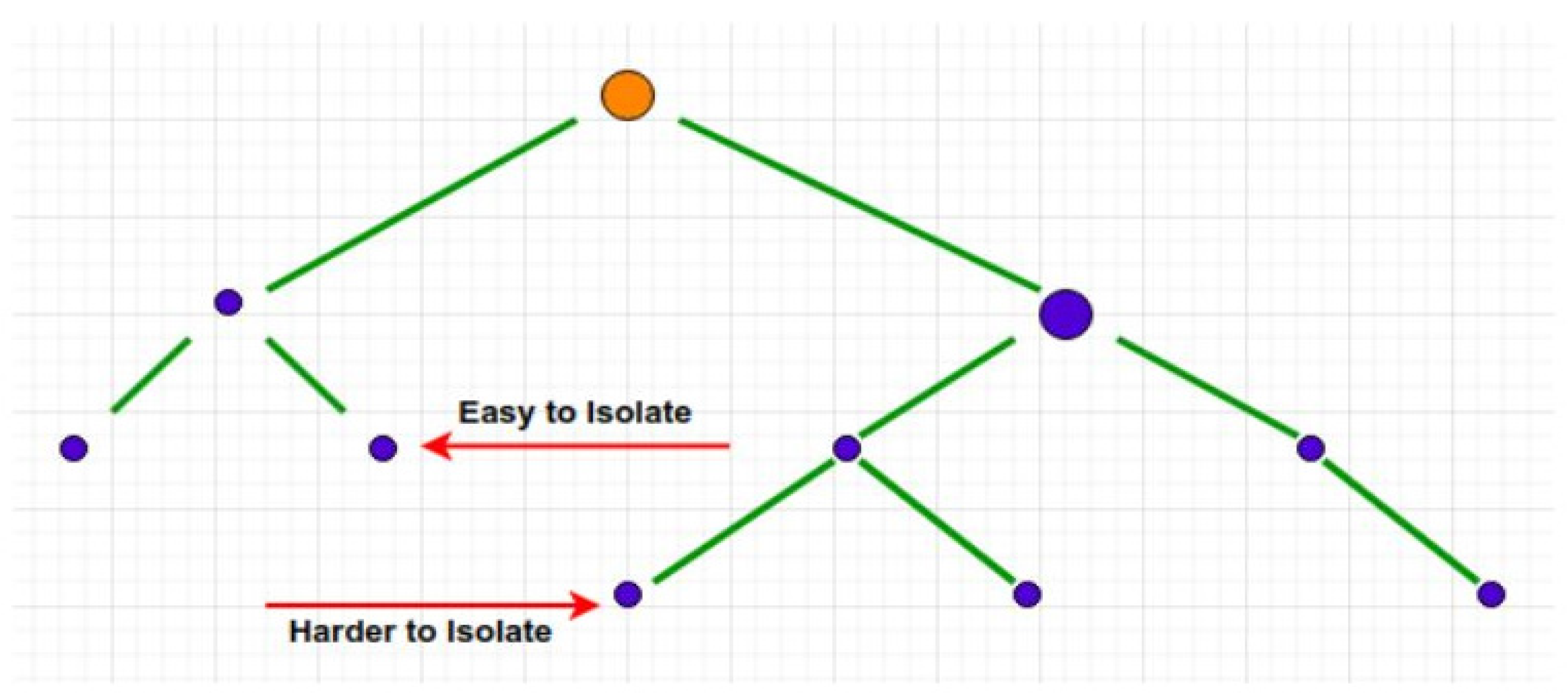
This algorithm uses two quantitative anomaly features to identify and detect outliers (impairment), (1) they are a minority consisting of fewer samples and (2) they have feature values that are very different from normal samples, and in other words, Abnormalities are “few and varied”, which makes them more susceptible to isolation than normal points. In this method, there are only two variables: the number of trees to construct and the size of the subsample. In this algorithm, the word isolated means separating one sample from the rest.

In a data-driven random tree, the partitioning of samples is repeated recursively until all samples are separated. This random partitioning produces shorter paths to anomalies because (a) fewer cases of anomalies result in fewer partitions—shorter paths in the tree structure, and (b) samples with recognizable feature values. Most likely, they are outliers. In summary, outlier data requires fewer partitions for separation and has a shorter path length.

The point x_i is a normal and normal point, because it is much more difficult to isolate it, and the point x_o is an unusual and abnormal point, and as it is clear in Figure 4, it will be easy to isolate point x_o and less partitions are needed. It is separated until this point.

The average path for point xi, which is a normal point, is much more than point xo (see Figure 5), that is, the length of the path for xi is much longer, and it is farther from the root, that is why it will be harder to separate it, and the point xo is also the roots are closer and it is easier to separate.

If T is a node of a splitting tree, then T is either an external node with no children, or an internal node with one test or exactly two daughter nodes $({\mathrm{T}}_l,{\mathrm{T}}_r)$. A test consists of a feature $q$ and a partition value $p$ such that the test $q<p$ divides the data points into ${\mathrm{T}}_l$ and ${\mathrm{T}}_r$. If a data sample $X=\left\{x_1,\dots ,x_n\right\}$ of $n$ samples from the d-variate distribution, to build a separation tree (iTree) that we recursively divide $X$ by randomly selecting the feature $q$ on a discrete value $p$ until: 1. The tree reaches its height 2. $\left|X\right|=1$ and 3. All data in $X$ have the same values.

An iTree is a suitable binary tree where each node in the tree has exactly zero or two daughter nodes. Assuming that all instances are distinct, when the iTree is fully grown, each instance is separated into an external node, in which case the number of external nodes is n and the number of internal nodes is $n-1$.

The total number of nodes in an iTree is $2n-1$. The task of anomaly detection is to provide a rating that reflects the extent of the anomaly. Therefore, one way to detect anomalies is to sort data points based on path length or anomaly scores. Anomalies are the points at the top of the list. We define the path length and anomaly score as follows, $h\left(x\right)$ The point $x$ is measured by the number of edges $x$ traverses an iTree from the root node until the traversal terminates at an external node.

$$c\left(n\right)=2H\left(n-1\right)-\left(2\right(n-1)/n)$$

(4)

where $H$ is a harmonic number that can be estimated by Euler’s constant number. Since $c\left(n\right)$ provide the mean of $h\left(x\right)$, n is used to normalize $h\left(x\right)$. The anomaly score $s$ of a sample $x$ is defined as follows:

$$s\left(x,n\right)=2^{-\frac{E\left(h\left(x\right)\right)}{c\left(n\right)}}$$

(5)

where $E\left(h\left(x\right)\right)$ is the mean of $h\left(x\right)$ extracted from a set of trees. In Equation (5):

$$\begin{gathered} \left(h\left(x\right)\right)\to c\left(n\right),s\to 0.5 \\ E\left(h\left(x\right)\right)\to 0,s\to 1 \\ E\left(h\left(x\right)\right)\to n-1,s\to 0 \end{gathered}$$

By establishing the following conditions using the anomaly score $s$, we can perform the following evaluation: $0<s\le 1$ for $0<h\left(x\right)\le n-1$.

(a)

Samples are definitely anomalies if they return s very close to $1$;

(b)

If the samples are much smaller than $0.5$, then they are quite safe to treat as normal samples;

(c)

If all samples return $s\approx 0.5$, then the entire sample really has no known anomalies.

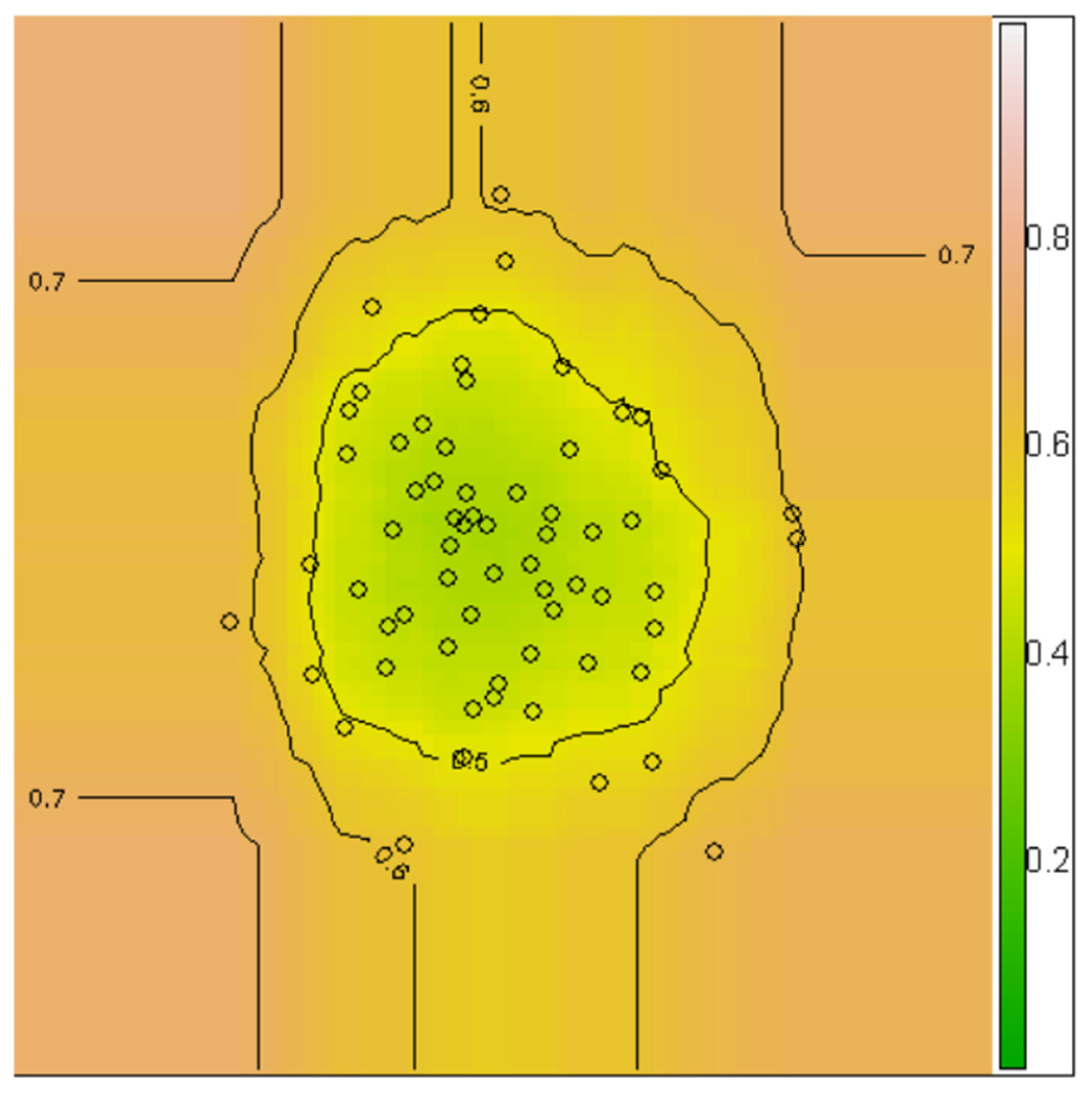
A contour of the anomaly score can be generated by passing a network sample through a set of separation trees, which facilitates a detailed analysis of the detection result. Figure 5 shows an example of such lines that allow the user to visualize and identify anomalies in the sample space. Using the contour, we can clearly identify three points where s ≥ 0.6 are potential anomalies.

As shown in Figure 6, normal and abnormal points are shown in a contour. The closer we get to the center of the contour, the number of healthy (normal) points increases, and the farther we go from the center, the number of abnormal points increases.

The brief explanation of this algorithm is that the data close to the root (abnormalities) are prone to isolation and separation, and the further away from the root, the more difficult it is to separate the data (normal and abnormal data) [20].

Isolation Forest (iForest) which detects anomalies purely based on the concept of isolation without employing any distance or density measure [20].

One of the algorithms used for data identification and classification is an unbalanced approach that focuses on the statistical characteristics of the data. This algorithm employs the construction of random trees to systematically analyze the dataset. The process begins by randomly initiating the construction of a tree. As the tree evolves, it gradually discerns distinctions within the data.

At each stage of tree construction, a random node is generated. Using a random feature, the algorithm segregates the data into two groups. As the data delves deeper into the tree’s structure, instances exhibiting abnormal characteristics are identified and separated from the normal data. This iterative process of tree construction and random feature extraction persists until all data points are effectively isolated from one another.

3.1.3. Minimum Covariance Determinant

The minimum covariance deterministic (MCD) estimator is one of the first highly robust dependent equivalent estimators of multivariate location and dispersion, and in addition, MCD has also been used to develop many robust multivariate techniques, including robust principal component analysis, factor analysis, and multiple regression is used. In the multivariate location and scatter settings, we assume that the data are stored in a matrix.

Where $={(x_1,\dots ,x_n)}^t$, $x_{\mathrm{i}}={(x_{i1},\dots ,x_{ip})}^t$ that n stands for the number of objects and $p$ for the number of variables. A classical tolerance ellipse is defined as a set of x-dimension p-points whose Mahalanobis distance.

$$MD\left(x\right)=\sqrt{{(x-\overline{x})}^t{S}^{-1}(x-\overline{x})} \mathrm{equals} \mathrm{to} \sqrt{x_{P,0.975}^2}$$

(6)

We denote $x_{P,\alpha }^2$ as the α-quantile of the $x^2$ p distribution. Mahalanobis distance $MD\left(x_i\right)$ should tell us how far $x_i$ is from the center of the cloud. which is $\overline{x}$ the sample mean and $S$ the sample covariance matrix.

In the description in Figure 7, we can see that the points that are closer to the root are easily separated from the rest of the data and these data are in an abnormal (unhealthy) state, and the further away from the root we become and distance, it becomes more difficult to separate the points and these data are in a normal (healthy) state and have a longer path to the root.

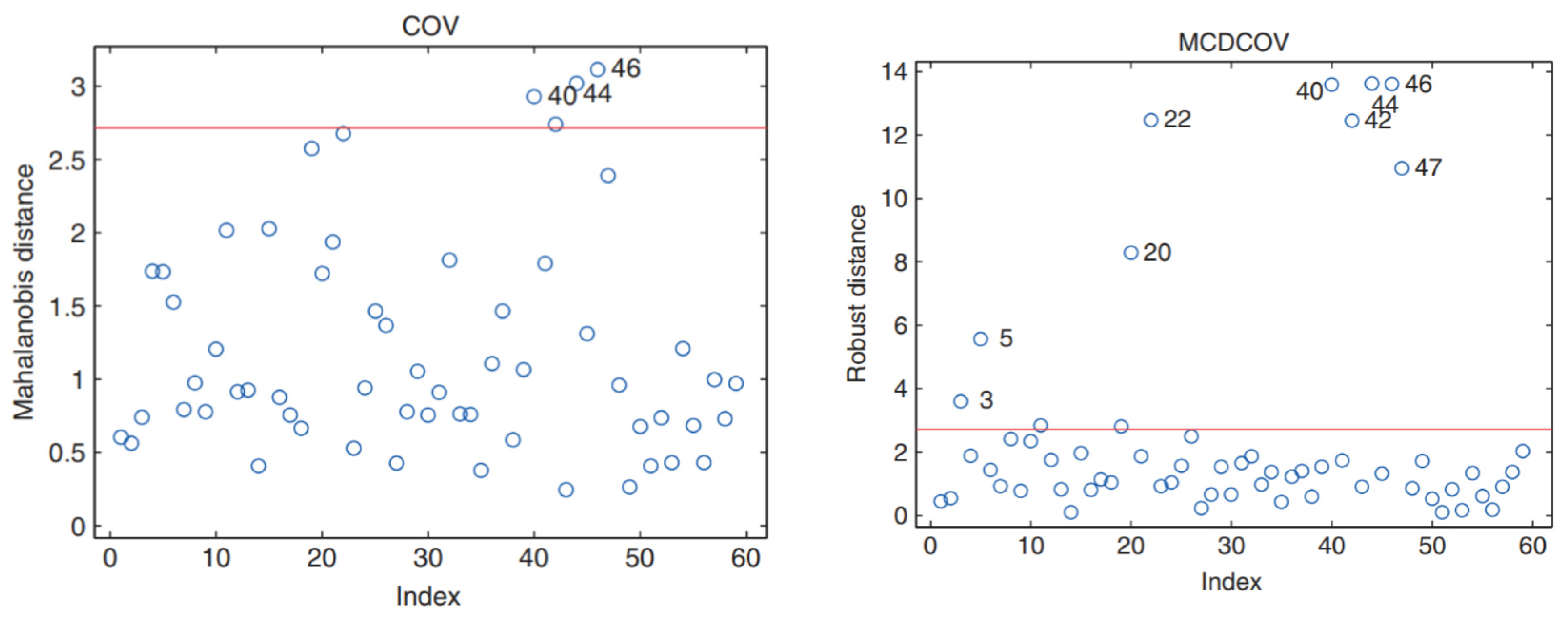
We see that this tolerance ellipse tries to include all observations. As a result, none of the Mahalanobis intervals, shown in the Figure 7, are exceptionally large, and only three observations are considered mild outliers. On the other hand, the resistive tolerance ellipse in Figure 1, which is based on resistive intervals, is much smaller and includes typical data points.

$$RD\left(x\right)=\sqrt{{(x-{\widehat{\mu }}_{MCD})}^t}{\sum }_{MCD}^{-1}(x-{\mu }_{MCD})$$

(7)

In this formula ${\widehat{\mu }}_{MCD}$, it indicates the estimation of the $MCD$ location and ${\sum }_{MCD}^{-1}$ the estimation of the $MCD$ covariance matrix. Using $RD\left(x\right)$, it is clearly seen in the figure that it performed better and identified eight outliers. This represents the masking effect: classical estimates can be so affected by outliers that diagnostic tools such as Mahalanobis intervals can no longer detect outliers. To obtain a reliable analysis of these data, robust estimators are needed that can withstand possible outliers. The location and dispersion $MCD$ estimator is such a robust estimator. And Robust distance has performed well to separate points from each other [21].

As shown in Figure 7, two lines (distance) have been drawn, and we can see that one of the lines performed much better than the other and was able to separate the points much better.

This algorithm starts by estimating the covariance matrix, which contains information about the probability distribution of the data. Subsequently, a subset of data are chosen to act as a representative sample, selected in a way that minimizes its covariance within the overall dataset. Using this representative data, the algorithm calculates an image of the dataset. This image, based on the analysis, reflects the normal distribution of the data. Finally, by comparing the dataset with the distribution represented by the chosen subset, anomalies or outlier data can be identified.

3.1.4. Local Outlier Factor

The detection of outliers is local and global in two ways, global outliers are points that are very far from other points and data, but local outlier detection covers a small subset of data points at a time. A local outlier is based on the probability that a data point pt is an outlier compared with its local neighborhood as measured by the k-nearest neighbors (kNN) algorithm.

Unsupervised outlier detection: Unsupervised algorithms do not require labels in the data and there is no discrimination between the training and testing datasets. Therefore, this mode is more flexible than the others. The basic idea of unsupervised outlier detection algorithms is to score data points based only on the basic features of the dataset. In general, the density or interval is used to provide an assessment of whether a data point is an inlier (normal) or outlier. This review is focused on unsupervised outlier detection.

As shown in Figure 8, the points are divided into three categories, normal points, abnormal points and local abnormal points. According to its formula, this algorithm will be able to identify local outliers in addition to outliers. General outliers are very far from normal points, but local outliers are close and similar to normal points, and it will be much more difficult to identify and separate them.

The distance between two data points p and o can be calculated using n-dimensional Euclidean space:

$$d\left(p,o\right)=\sqrt{\sum _{i=1}^n{(p_i-o_i)}^2}$$

(8)

Here, the meaning of k-Nearest Neighbors (kNN) of p is any data point q whose distance to the p data point is not greater than the k-distance ($p$). Those k-Nearest Neighbors of $q$ form the so-called k-distance neighborhood of $p$, as described in Equation (9):

$$N_{k-distance\left(p\right)}\left(p\right)=\left\{q\in D\backslash \left\{p\right\}\left|d\right(p,q)\le k-distance\left(p\right)\right\}$$

(9)

Let $k$ be a positive integer. The reachable distance of a data point $p$ with respect to the data point $o$ is defined in the following relation:

$$reach-{dist}_k\left(p,o\right)=max\left\{k-distance\left(o\right),d(p,o)\right\}$$

(10)

In density-based clustering algorithms, two parameters are used to define the concept of density: (1) MinPts for the minimum number of data points and (2) a volume and, therefore, the local reach density $\left(Lrd\right)$ of the data point p is defined in the following Equation (11):

$${Lrd}_{MinPts}\left(p\right)=1/\left(\frac{\sum _{0\in N_{MinPts\left(p\right)}}reach-{dist}_{MinPts}(p,o)}{\left|MinPts\left(p\right)\right|}\right)$$

(11)

In the above relation, first, the average access distance is calculated based on the number of $MinPts$ of the nearest neighbors of the data point $p$. Its inversion then produces the local reach density $\left(Lrd\right)$ of the data point $p$. With all the work mentioned above, the $LOF$ score of a data point $p$ can be calculated through the following Equation (12):

$${LOF}_{MinPts}\left(p\right)=\frac{\sum _{n\in N_{MinPts\left(p\right)}}\frac{{Lrd}_{MinPts}\left(o\right)}{{Lrd}_{MinPts}\left(p\right)}}{\left|N_{MinPts}\left(p\right)\right|}$$

(12)

The above equation calculates the average ratio of local access density of data point $p$ and $MinPts$-nearest neighbors of data point $p$. Finally, a $LOF$ score is assigned to each data point. A threshold score $\theta$ is used to determine whether a data point $p$ is an outlier. The strength of $LOF$ is that it can identify local density and determine local outliers. Its disadvantages are that it requires a long execution time and is sensitive to the value of the minimum score [22,23].

In this algorithm, the process of anomaly detection involves several steps. Firstly, for each point, its neighbors are identified based on their distances from the target point. Subsequently, the local density is computed for each point, representing the density in the vicinity of the target point. Following this, by comparing the local density of neighbors with the density of the target point, the point is classified as either a normal point or an anomaly point. The threshold for the Local Outlier Factor (LOF) is set at one, and if it exceeds this value, the point is considered an anomaly.

While this method can yield satisfactory results in feature spaces with low dimensionality (few features), its reliability tends to diminish as the number of features increases, a phenomenon commonly referred to as the curse of dimensionality.

The local outlier factor, or LOF for short, is a technique designed to capitalize on the notion of nearest neighbors for outlier detection. Each example receives a score reflecting its degree of isolation or likelihood of being an outlier, determined by the size of its local neighborhood. Examples with the highest scores are considered more likely to be outliers.

4. Description of the Dataset and Benchmark Structures Utilized in the Study

4.1. IASC-ASCE Laboratory Structure

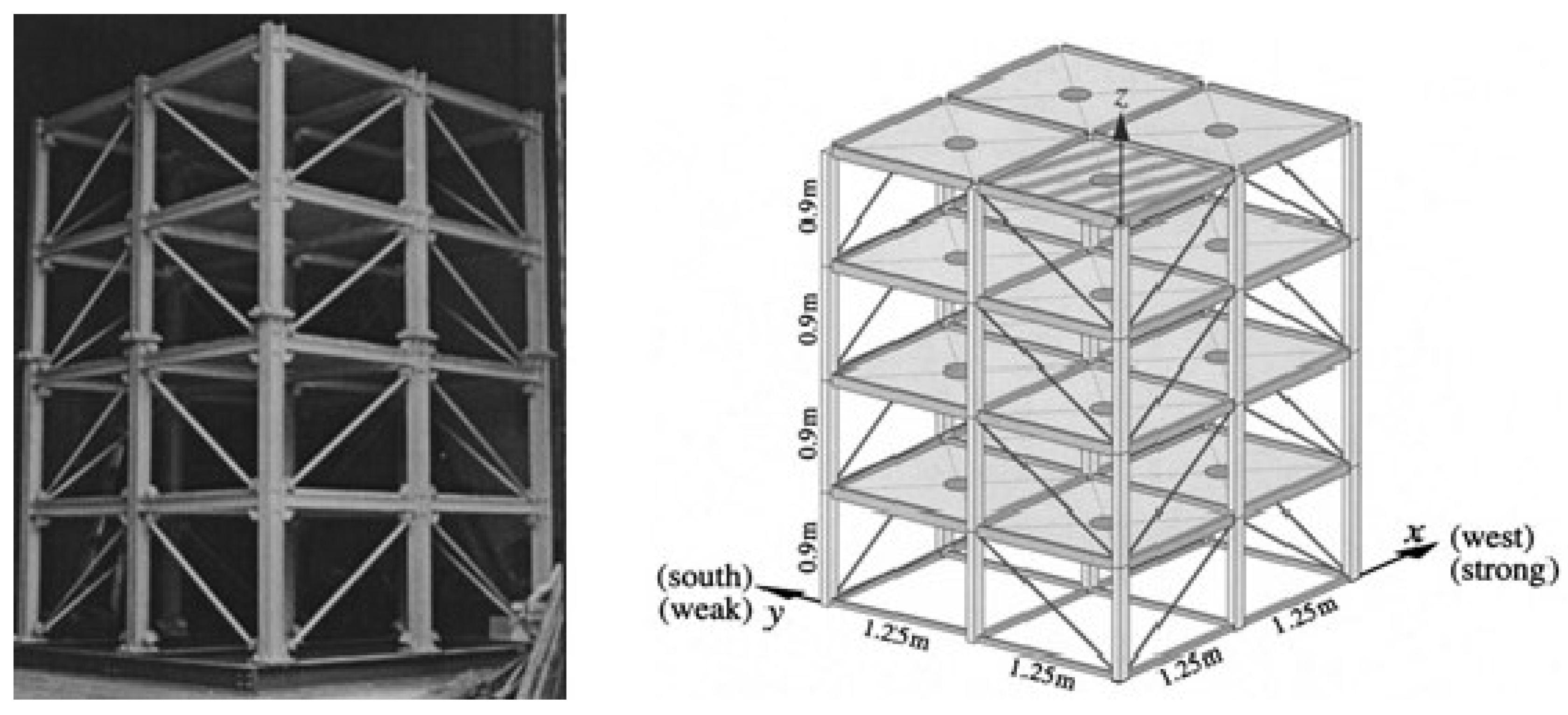
The structure depicted in Figure 9 is a four-story steel frame model with a two-by-two bay configuration, located at the Earthquake Engineering Research Laboratory at the University of British Columbia (UBC). The plan dimensions are 2.5 m by 2.5 m, and the structure has a height of 3.6 m.

Two finite element models were developed based on this structure to generate simulated response data. The first model is a 12-degree-of-freedom and shear model of the building, limiting all motion except for two horizontal translations and one rotation per floor. The second model is a 120-degree-of-freedom configuration that only requires horizontal translational motion and internal rotation at the floor nodes. 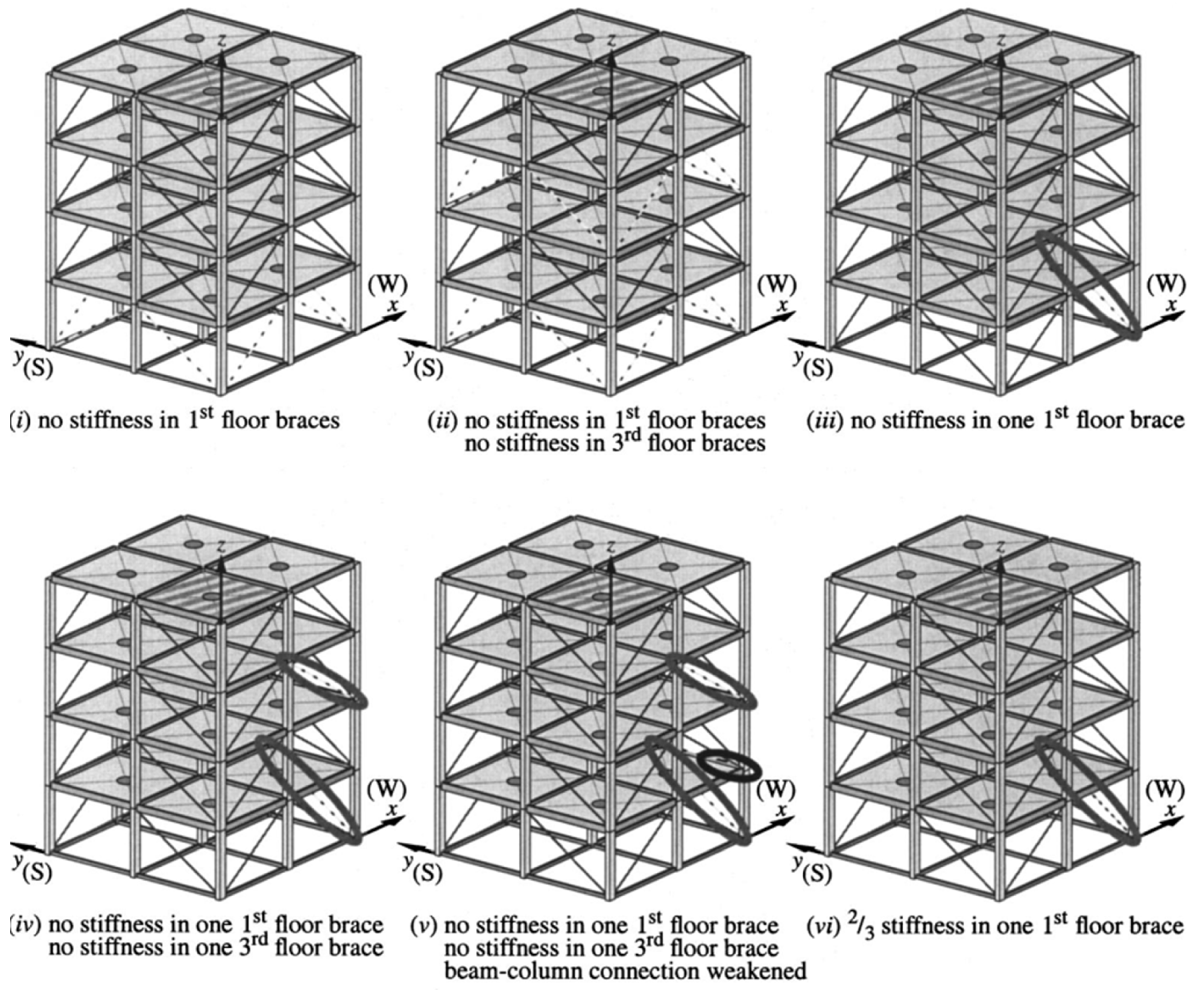Figure 10 illustrates six damage modes for this structure.

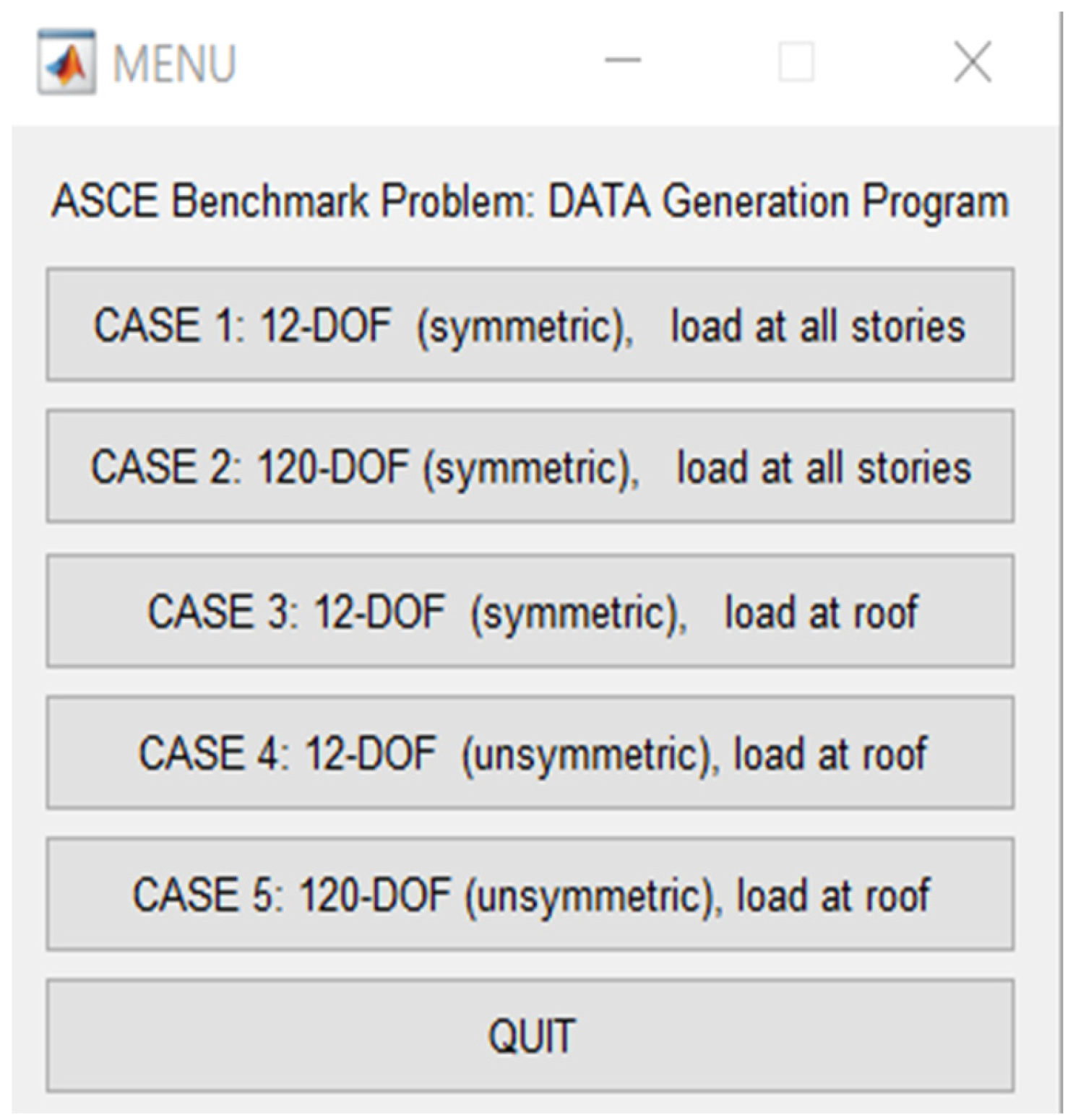
The code for this structure is written in MATLAB software (version 20). By running and analyzing the structure in MATLAB, acceleration data for accelerometers is obtained. In the initial analysis of this structure, we selected a symmetrical 12-degree-of-freedom structure with load distribution across all floors.

The benchmark structure exhibits five modes (refer to Figure 11), where two modes are associated with times when the roof is not considered rigid, leading to an increase in the number of degrees of freedom to 120. This configuration is typically used for research purposes. In other cases, when considering the roofs as rigid, the structure has 12 degrees of freedom. Another distinction between the states of the structure is that some analyses are conducted symmetrically, while others are asymmetric. However, we opted for a mode where the structure is symmetrical in all directions, with loads applied to all stories, resulting in a structure with 12 degrees of freedom.

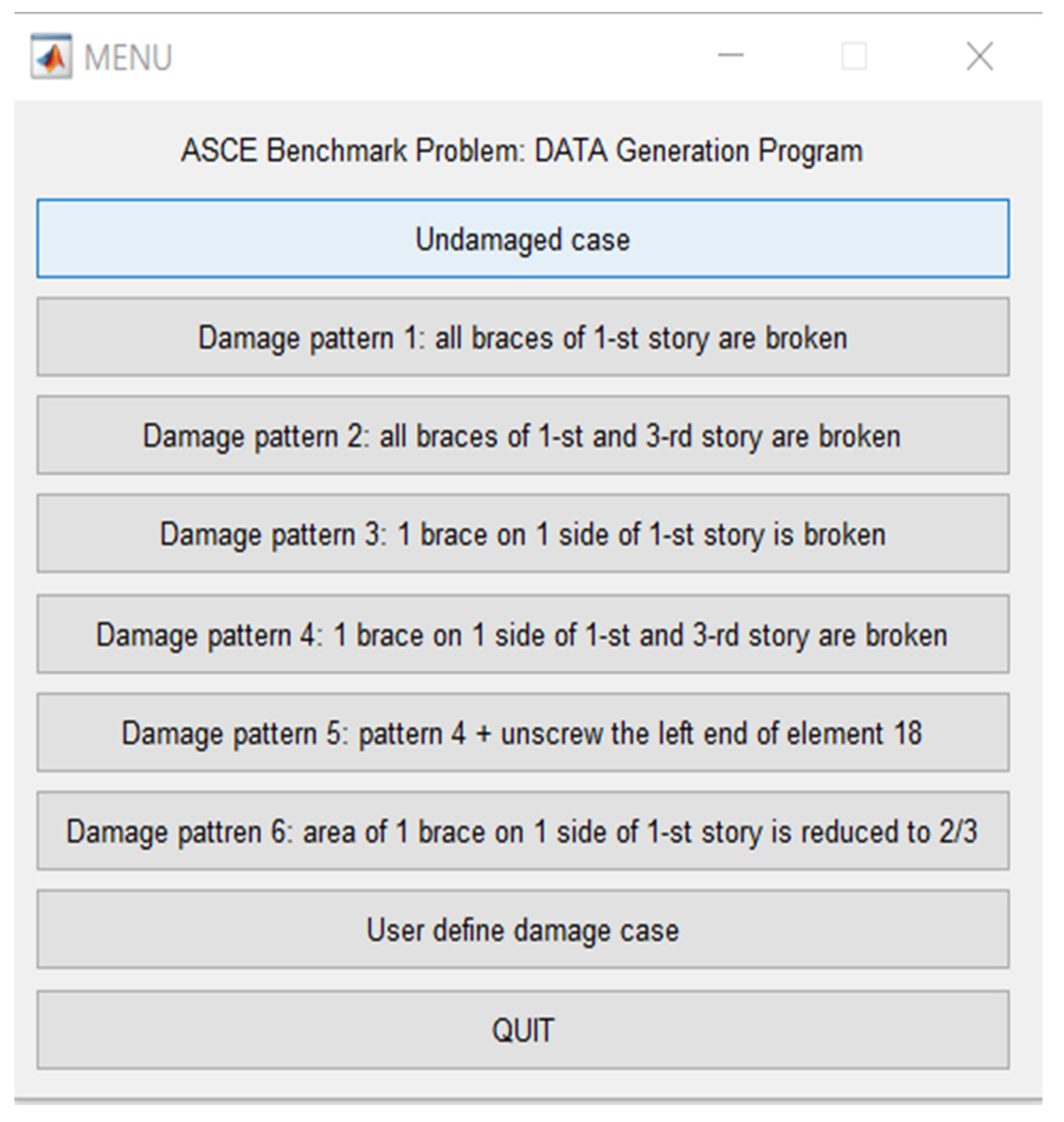
In the second step, we need to select the desired cases, which include 7 modes. The first mode represents an undamaged scenario, and the remaining 6 modes correspond to different damage scenarios, all of which have been included.

In summary, this structure exhibits 6 states of damage and one state where the structure is undamaged. By selecting each of these modes, various damage states can be thoroughly and comprehensively illustrated, as shown in Figure 12.

In the third step, we are required to select the preferred analysis method. It is worth mentioning that certain methods may necessitate the installation of Toolbax; however, we opted for Isim. Essentially, we need to specify the analysis type and choose one of the available methods for conducting the structural analysis (refer to Figure 13).

In the fourth step, it is crucial to specify the damping level, time step, analysis duration, along with the load magnitude, and assign a name to the analysis. As depicted in Figure 14, various values need to be considered for the analysis, including a damping value of 0.01, a time step equal to 0.001, an analysis duration of 40 s, a noise level of 10%, and a load magnitude of 150. These characteristics are essential for a comprehensive analysis of the structure.

After implementing the required and desired modifications and running the analysis, a data frame is generated with 16 columns. Each column represents the acceleration readings from an accelerometer. Additionally, considering the time steps and the analysis duration set at 40 s, the data frame consists of 40,001 rows, as detailed in reference [24].

4.2. Yonghe Bridge in China

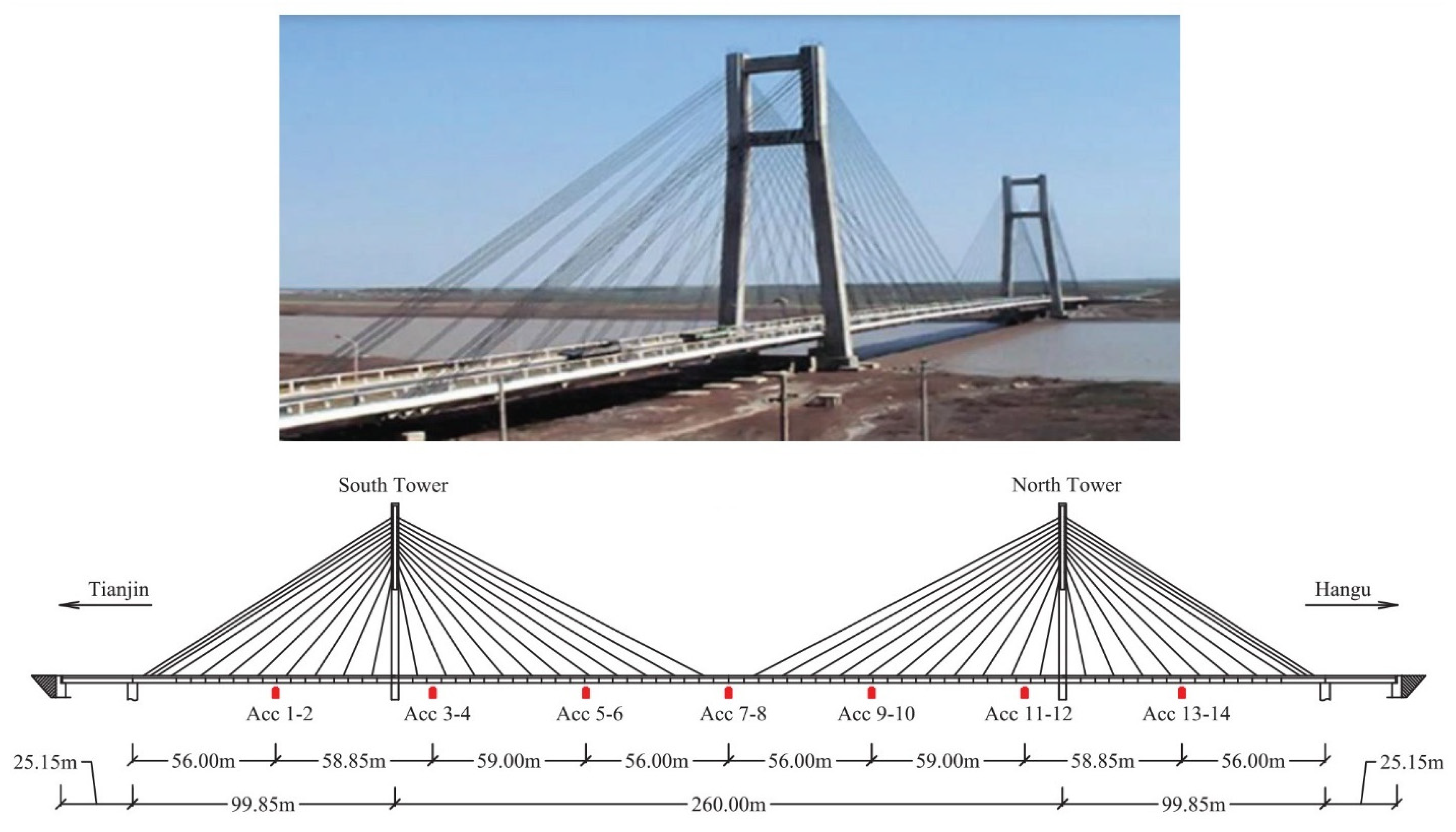
The Yonghe Bridge, located in Tianjin, China, is a cable-stayed bridge depicted in Figure 15. This authentic cable-stayed bridge boasts a main span of 260 m and two side spans measuring 25.15 m and 99.85 m, respectively. With a total length of 510 m and a width of 11 m (9 m for vehicles and 2 m for pedestrians), the bridge features a concrete tower composed of two transverse beams, each standing at a height of 60.5 m. These beams are consistently formed through cast-in-place joints, connecting the ends of the beams, and creating transversely reinforced diaphragms.

After 19 years in operation, the bridge exhibited cracks with a maximum width of 2 cm at the bottom of a beam section along the middle span. These cracks were likely induced by overloaded vehicles, surpassing the weight and volume originally anticipated in the design. Additionally, the supporting cables, particularly those near the anchors, experienced severe corrosion.

The placement of accelerometers and other tools, along with the dimensions of different parts of the bridge, is outlined in Figure 15. Repairs were conducted between 2005 and 2007, involving the re-insertion of the beam above the mid-span and the replacement of all fixed cables. Throughout the repair and reconstruction process, a sophisticated SHM system was designed for the bridge and implemented by the SMC Center at Harbin Institute of Technology.

In this study, acceleration and environmental conditions measured by the SHM system on 1 January,17 January, 3 February, 19 March, 30 March, 9 April, 5 May, 18 May, 31 May, 7 June, 16 June, and 31 July, collected in 2008, were selected to represent the bridge’s time history from a healthy to a damaged state. For acceleration data, each file contains a total of 17 columns. The first column indicates the measurement time, while the subsequent 16 columns display the acceleration time history collected using 14 uniaxial accelerometers installed on the bridge deck and 1 dual-axis accelerometer positioned on top of the south tower. The acceleration sampling frequency is 100 Hz.

Due to the substantial volume of data, the numbers stored in the MATLAB file are actual readings obtained from the accelerometers, reflecting the real nature of the structure. With a dataset spanning 9 months for this bridge, 4 months of it have been utilized for coding. The selection process involved considering the data from the first month as representative of the healthy state. As time progressed and incidents occurred, subsequent months’ data were used to depict the damaged state.

Specifically, January data were employed to depict the healthy state, while July, March, and June were chosen to represent the first, second, and third instances of damage, respectively. It is noteworthy that managing this dataset involves handling a substantial volume of data [25].

5. The Research Methodology

In the initial stages, the necessity arose to convert data from both structures, initially stored in MATLAB software, into CSV files for seamless integration into our programming environment. The subsequent step involved meticulous preprocessing to clean the data by removing empty entries and other artifacts from the dataset.

The data for both benchmark structures primarily comprised acceleration readings. The acceleration data for the first structure was obtained by executing the model in MATLAB, whereas the accelerations for the second structure were stored in an extensive MATLAB file over several months. However, due to the real-world nature of the structure, this file was exceptionally large, containing millions of acceleration data points. This posed significant computational challenges, necessitating robust hardware, which emerged as a primary constraint in our research.

Following the conversion and import of data into the Python programming language, utilizing the Jupyter programming environment, we proceeded with coding. In the initial coding step, we imported the requisite algorithms and criteria, inputting the structure’s accelerations into the coding environment. Subsequently, we determined the volume of data to be used for the first structure. To mitigate computational load, we worked with data in various states: healthy and damaged. For a comprehensive understanding of algorithm behavior, we experimented with different distributions, including:

• 90% healthy data and 10% damaged data;
• 75% healthy data and 25% damaged data;
• Equal proportions of healthy and damaged data.

However, for the second structure, due to the computational intensity involved, we opted for the first distribution from the aforementioned scenarios, specifically, 90% healthy data and 10% damaged data. For each algorithm, 70% of the total data served as training data, while the remaining 30% was allocated to the test mode.

One of the parameters employed is “contamination”, which denotes the degree of impurity in the dataset, specifically the proportion of outliers. This parameter is utilized during the fitting process to determine the threshold for the scores assigned to the samples.

Another utilized parameter is “random_state”. If we set the value of this parameter to any integer (whether 1, 4, 42, etc.), then in each iteration when the algorithm is repeated to generate the model, the data are divided into training and test sets in equal proportion to the previous step. For example, in each step, 0.7 of the data are randomly assigned to the training set, and 0.3 is allocated to the test set.

To evaluate algorithm performance, we utilized four key criteria: F1-Score, Accuracy Score, Precision Score, and Recall Score.

5.1. Accuracy Score

Perhaps the first and simplest criterion that we go to is the accuracy criterion, which is equal to the number of cases that we correctly predicted, which we call True Positive, divided by the total number of predictions that have been made.

$$Accuracy=\frac{TP+TN}{TP+TN+FP+FN}$$

5.2. F1 Score or F-Measure Evaluation Criteria

The F1 criterion is a suitable criterion for evaluating the accuracy of an experiment. This measure considers Precision and Recall together. The F1 criterion is one at best and zero at worst.

$$F1-Score=2\times \frac{Precision . Recall}{Precision+Recall}$$

5.3. Precision Measure

The maximum value of this criterion is 1 or 100% and its minimum value is zero, and the more cases that the program has predicted incorrectly, which we call False Positive, compared with true or True Positive predictions, the lower the Precision value will be. In the following formula, TP stands for True Positive and FP stands for False Positive.

$$Precision=\frac{TP}{TP+FP}$$

5.4. Recall Score

The maximum value of this criterion is 1 or 100% and its minimum value is zero, and the more cases that we expected were predicted but the program did not predict, which we call False Negative, than the true or True Positive predictions, the lower the Recall value will be.

$$Recall=\frac{TP}{TP+FN}$$

It is commonly utilized to assess the effectiveness of classification models, particularly those tasked with predicting a categorical label for each input instance. The matrix discloses the counts of true positives (TP), true negatives (TN), false positives (FP), and false negatives (FN) generated by the model during the testing phase.

For a more detailed insight into how the data are classified, the confusion matrix is employed. The confusion matrix is an N × N grid, where N signifies the number of classes; in a binary classification setting, such as the one described, there are two classes—one for healthy data and the other for unhealthy data—resulting in a 2 × 2 matrix. This matrix forms the basis for computing various evaluation metrics. The entries on the main diagonal denote correctly classified instances, while those on the off-diagonal indicate misclassifications. Label number 0 is assigned to damaged data, and label number 1 is assigned to healthy data. The horizontal axis represents the algorithm’s performance, while the vertical axis signifies the actual values. The confusion matrix is presented in

Table 1. Confusion matrix.

		Predicted Label
		0	1
True Label	0	TN	FP
	1	FN	TP

below.

6. Results and Performance of Algorithms on Two Benchmark Structures

6.1. The Results of the First Structure (IASC-ASCE Laboratory Structure)

In this numerical model, structural accelerations obtained in MATLAB, considering various values, serve as inputs for the structure to perform damage detection. Since 16 sensors (4 sensors on each floor) are employed in the structure, a total of 16 columns are generated in the MATLAB output, accounting for time steps, load values, displacement values, and other parameters. Each of these columns represents the structural acceleration under a specific excitation at each moment (second). The numbers derived in the MATLAB output correspond to the structural acceleration values utilized as inputs for machine learning models.

After coding to evaluate accuracy, precision, and the performance of these algorithms for 6 different damage patterns and 3 distinct data distribution scenarios, 4 specific criteria we apply. These results are presented individually for each damage pattern.

Scenario 1: The healthy data rate is 90%, and the unhealthy data rate is 10%.

Scenario 2: The healthy data rate is 75%, and the unhealthy data rate is 25%.

Scenario 3: The healthy data rate is 50%, and the unhealthy data rate is 50%.

The results for scenarios are provided in the following

Table 2. Results of the algorithms for damage pattern 1 and scenario 1.

	One-Class Support Vector Machines	Isolation Forest	Minimum Covariance Determinant	Local Outlier Factor
F1-Score	0.018	0.090	0.074	0.078
Accuracy Score	0.890	0.822	0.818	0.814
Precision Score	0.081	0.091	0.076	0.077
Recall Score	0.010	0.088	0.073	0.078

,

Table 3. Results of the algorithms for damage pattern 2 and scenario 1.

	One-Class Support Vector Machines	Isolation Forest	Minimum Covariance Determinant	Local Outlier Factor
F1-Score	0.015	0.067	0.086	0.082
Accuracy Score	0.887	0.820	0.810	0.816
Precision Score	0.056	0.068	0.082	0.363
Recall Score	0.008	0.066	0.090	0.432

,

Table 4. Results of the algorithms for damage pattern 3 and scenario 1.

	One-Class Support Vector Machines	Isolation Forest	Minimum Covariance Determinant	Local Outlier Factor
F1-Score	0.339	0.330	0.510	0.395
Accuracy Score	0.910	0.845	0.880	0.861
Precision Score	0.623	0.290	0.422	0.363
Recall Score	0.233	0.376	0.633	0.432

,

Table 5. Results of the algorithms for damage pattern 4 and scenario 1.

	One-Class Support Vector Machines	Isolation Forest	Minimum Covariance Determinant	Local Outlier Factor
F1-Score	0.390	0.330	0.510	0.420
Accuracy Score	0.915	0.850	0.880	0.870
Precision Score	0.702	0.294	0.422	0.375
Recall Score	0.268	0.378	0.633	0.475

,

Table 6. Results of the algorithms for damage pattern 5 and scenario 1.

	One-Class Support Vector Machines	Isolation Forest	Minimum Covariance Determinant	Local Outlier Factor
F1-Score	0.350	0.320	0.510	0.163
Accuracy Score	0.911	0.843	0.880	0.830
Precision Score	0.643	0.281	0.421	0.161
Recall Score	0.238	0.367	0.643	0.166

and

Table 7. Results of the algorithms for damage pattern 6 and scenario 1.

	One-Class Support Vector Machines	Isolation Forest	Minimum Covariance Determinant	Local Outlier Factor
F1-Score	0.066	0.140	0.141	0.163
Accuracy Score	0.890	0.830	0.831	0.830
Precision Score	0.210	0.140	0.141	0.161
Recall Score	0.040	0.140	0.141	0.166

. (In the tables below, green color indicates the best performance).

The most important metric for evaluating algorithm performance is the F1-score.

As evident from the tables highlighted in green, except for damage pattern 1 where three algorithms are closely matched, with a slight difference, the Isolation Forest algorithm outperformed. However, in other scenarios, the Minimum Covariance Determinant algorithm demonstrated better performance.

The results for two additional scenarios are provided in the following

Table 8. Results of the algorithms for damage pattern 1 and scenario 2.

	One-Class Support Vector Machines	Isolation Forest	Minimum Covariance Determinant	Local Outlier Factor
F1-Score	0.030	0.126	0.110	0.120
Accuracy Score	0.743	0.695	0.696	0.693
Precision Score	0.255	0.223	0.203	0.212
Recall Score	0.014	0.088	0.074	0.083

,

Table 9. Results of the algorithms for damage pattern 2 and scenario 2.

	One-Class Support Vector Machines	Isolation Forest	Minimum Covariance Determinant	Local Outlier Factor
F1-Score	0.019	0.091	0.122	0.121
Accuracy Score	0.740	0.693	0.695	0.693
Precision Score	0.168	0.176	0.220	0.216
Recall Score	0.010	0.061	0.085	0.090

,

Table 10. Results of the algorithms for damage pattern 3 and scenario 2.

	One-Class Support Vector Machines	Isolation Forest	Minimum Covariance Determinant	Local Outlier Factor
F1-Score	0.365	0.421	0.646	0.400
Accuracy Score	0.800	0.760	0.830	0.770
Precision Score	0.820	0.530	0.675	0.574
Recall Score	0.234	0.350	0.619	0.303

,

Table 11. Results of the algorithms for damage pattern 4 and scenario 2.

	One-Class Support Vector Machines	Isolation Forest	Minimum Covariance Determinant	Local Outlier Factor
F1-Score	0.388	0.400	0.652	0.410
Accuracy Score	0.800	0.760	0.830	0.771
Precision Score	0.840	0.523	0.700	0.575
Recall Score	0.253	0.319	0.640	0.316

,

Table 12. Results of the algorithms for damage pattern 5 and scenario 2.

	One-Class Support Vector Machines	Isolation Forest	Minimum Covariance Determinant	Local Outlier Factor
F1-Score	0.391	0.452	0.645	0.400
Accuracy Score	0.802	0.770	0.830	0.800
Precision Score	0.852	0.561	0.673	0.560
Recall Score	0.253	0.380	0.619	0.312

and

Table 13. Results of the algorithms for damage pattern 6 and scenario 2.

	One-Class Support Vector Machines	Isolation Forest	Minimum Covariance Determinant	Local Outlier Factor
F1-Score	0.080	0.210	0.300	0.213
Accuracy Score	0.750	0.712	0.724	0.718
Precision Score	0.481	0.335	0.404	0.353
Recall Score	0.042	0.152	0.222	0.153

.

In this scenario, similar to the first damage pattern where the results of three algorithms were close, the Minimum Covariance Determinant algorithm exhibited better performance in the remaining cases.

The following

Table 14. Results of the algorithms for damage pattern 1 and scenario 3.

	One-Class Support Vector Machines	Isolation Forest	Minimum Covariance Determinant	Local Outlier Factor
F1-Score	0.029	0.150	0.150	0.139
Accuracy Score	0.500	0.500	0.500	0.490
Precision Score	0.471	0.500	0.500	0.430
Recall Score	0.015	0.088	0.088	0.083

,

Table 15. Results of the algorithms for damage pattern 2 and scenario 3.

	One-Class Support Vector Machines	Isolation Forest	Minimum Covariance Determinant	Local Outlier Factor
F1-Score	0.023	0.114	0.145	0.130
Accuracy Score	0.500	0.484	0.494	0.484
Precision Score	0.363	0.401	0.500	0.413
Recall Score	0.012	0.066	0.086	0.077

,

Table 16. Results of the algorithms for damage pattern 3 and scenario 3.

	One-Class Support Vector Machines	Isolation Forest	Minimum Covariance Determinant	Local Outlier Factor
F1-Score	0.380	0.524	0.719	0.301
Accuracy Score	0.610	0.650	0.760	0.560
Precision Score	0.923	0.799	0.860	0.722
Recall Score	0.240	0.390	0.618	0.190

,

Table 17. Results of the algorithms for damage pattern 4 and scenario 3.

	One-Class Support Vector Machines	Isolation Forest	Minimum Covariance Determinant	Local Outlier Factor
F1-Score	0.406	0.520	0.732	0.320
Accuracy Score	0.620	0.644	0.770	0.566
Precision Score	0.930	0.799	0.872	0.750
Recall Score	0.260	0.384	0.631	0.200

,

Table 18. Results of the algorithms for damage pattern 5 and scenario 3.

	One-Class Support Vector Machines	Isolation Forest	Minimum Covariance Determinant	Local Outlier Factor
F1-Score	0.420	0.510	0.726	0.310
Accuracy Score	0.630	0.640	0.763	0.565
Precision Score	0.932	0.783	0.860	0.748
Recall Score	0.271	0.380	0.629	0.195

and

Table 19. Results of the algorithms for damage pattern 5 and scenario 3.

	One-Class Support Vector Machines	Isolation Forest	Minimum Covariance Determinant	Local Outlier Factor
F1-Score	0.097	0.246	0.343	0.227
Accuracy Score	0.516	0.528	0.560	0.525
Precision Score	0.720	0.611	0.679	0.611
Recall Score	0.052	0.154	0.229	0.139

correspond to a scenario where the values of healthy and unhealthy data are equal.

Overall, in the first structure (numerical model), the Minimum Covariance Determinant algorithm has demonstrated superior performance.

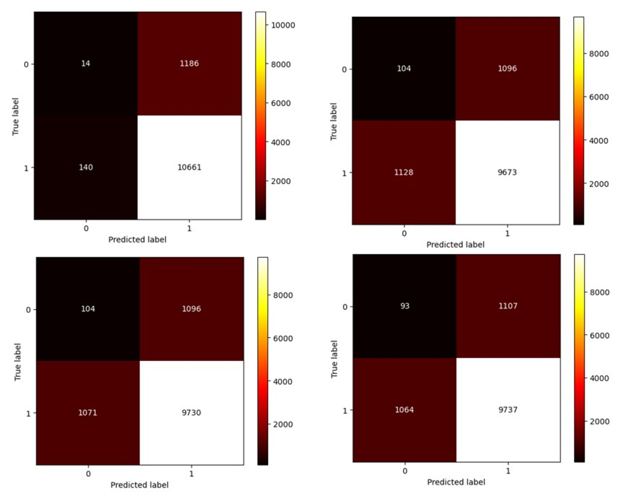
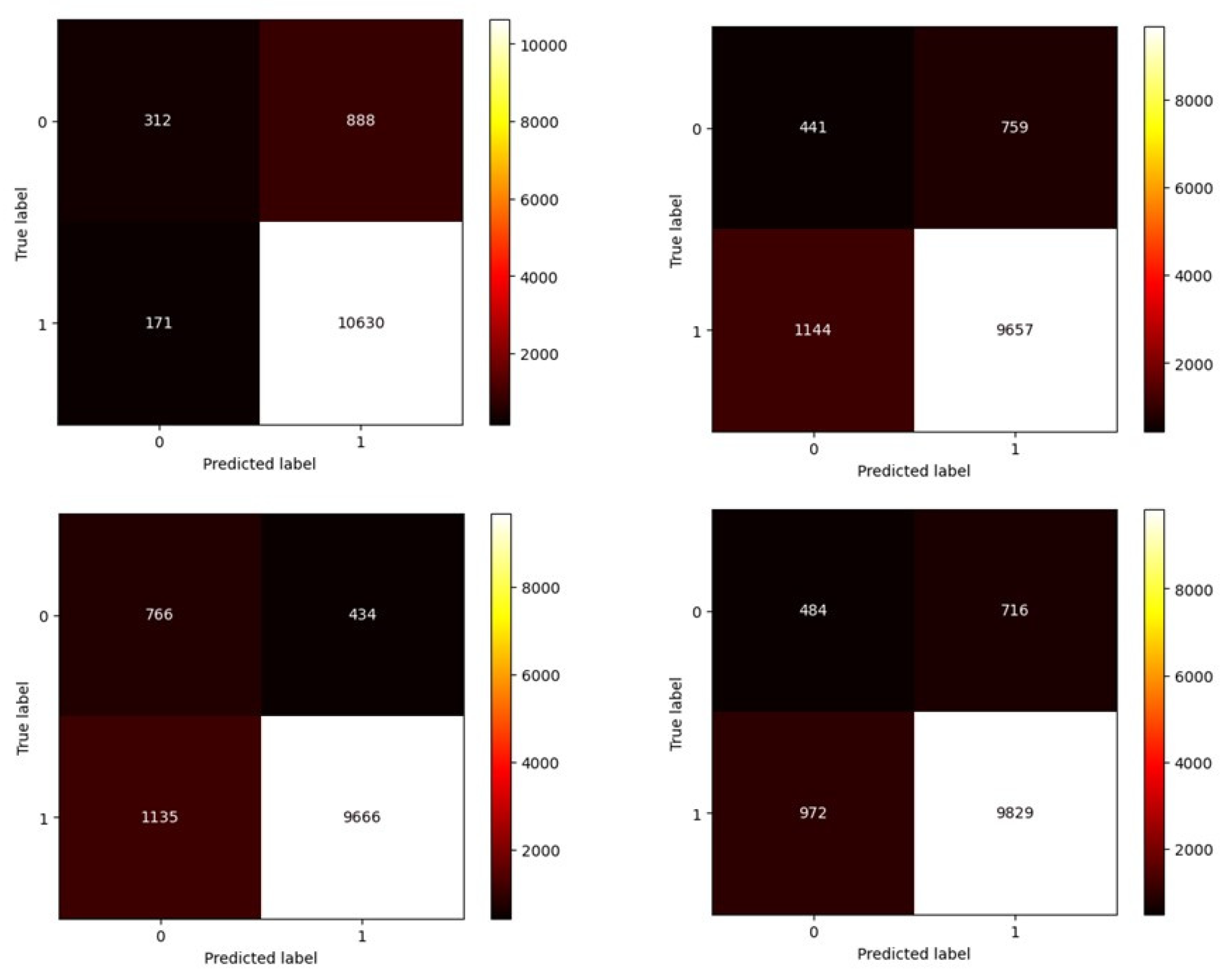
For a better understanding of classification and anomaly detection, a confusion matrix for the first case is presented in Figure 16, Figure 17 and Figure 18 below as an example.

The number 0 indicates the damaged state, and the number 1 indicates the healthy state. In this confusion matrix, the vertical axis represents the actual data, while the horizontal axis represents the model’s predicted data.

6.2. The Second Structure (Yonghe Bridge)

In this second structure (actual bridge), the data available consists of the genuine and real accelerations of the bridge under various loads during different days and months. These data serve as inputs to our machine learning models.

The following

Table 20. Results and performance of the algorithms for Damage Pattern 1.

	One-Class Support Vector Machines	Isolation Forest	Minimum Covariance Determinant	Local Outlier Factor
F1-Score	0.185	0.485	0.450	0.154
Accuracy Score	0.902	0.871	0.865	0.830
Precision Score	0.554	0.403	0.378	0.151
Recall Score	0.111	0.609	0.546	0.160

,

Table 21. Results and performance of the algorithms for Damage Pattern 2.

	One-Class Support Vector Machines	Isolation Forest	Minimum Covariance Determinant	Local Outlier Factor
F1-Score	0.030	0.130	0.116	0.195
Accuracy Score	0.893	0.823	0.822	0.833
Precision Score	0.146	0.128	0.115	0.188
Recall Score	0.015	0.132	0.117	0.202

and

Table 22. Results and performance of the algorithms for Damage Pattern 3.

	One-Class Support Vector Machines	Isolation Forest	Minimum Covariance Determinant	Local Outlier Factor
F1-Score	0.070	0.191	0.160	0.178
Accuracy Score	0.940	0.868	0.865	0.870
Precision Score	0.192	0.141	0.119	0.133
Recall Score	0.043	0.295	0.243	0.268

illustrate diverse outcomes for the Yonghe Bridge under conditions where the healthy data rate is 90%, and the unhealthy data rate is 10%.

In this study, acceleration and environmental conditions were collected by the SHM system on 1 January, 17 January, 3 February, 19 March, 30 March, 9 April, 5 May, 18 May, 31 May, 7 June, 16 June, and 31 July 2008. These data were chosen to represent the time history of the bridge, ranging from a healthy to a damaged state. Each file contains 17 columns for acceleration data. The first column indicates the measurement time, while the subsequent 16 columns depict the time history of acceleration collected using 14 uniaxial accelerometers installed on the bridge deck and 1 dual-axis accelerometer installed on top of the south tower. The acceleration data are sampled at a frequency of 100 Hz.

The data collected in January represents the healthy state, July corresponds to the first injury, March signifies the second injury, and June represents the third injury (Note: There is a large volume of data).

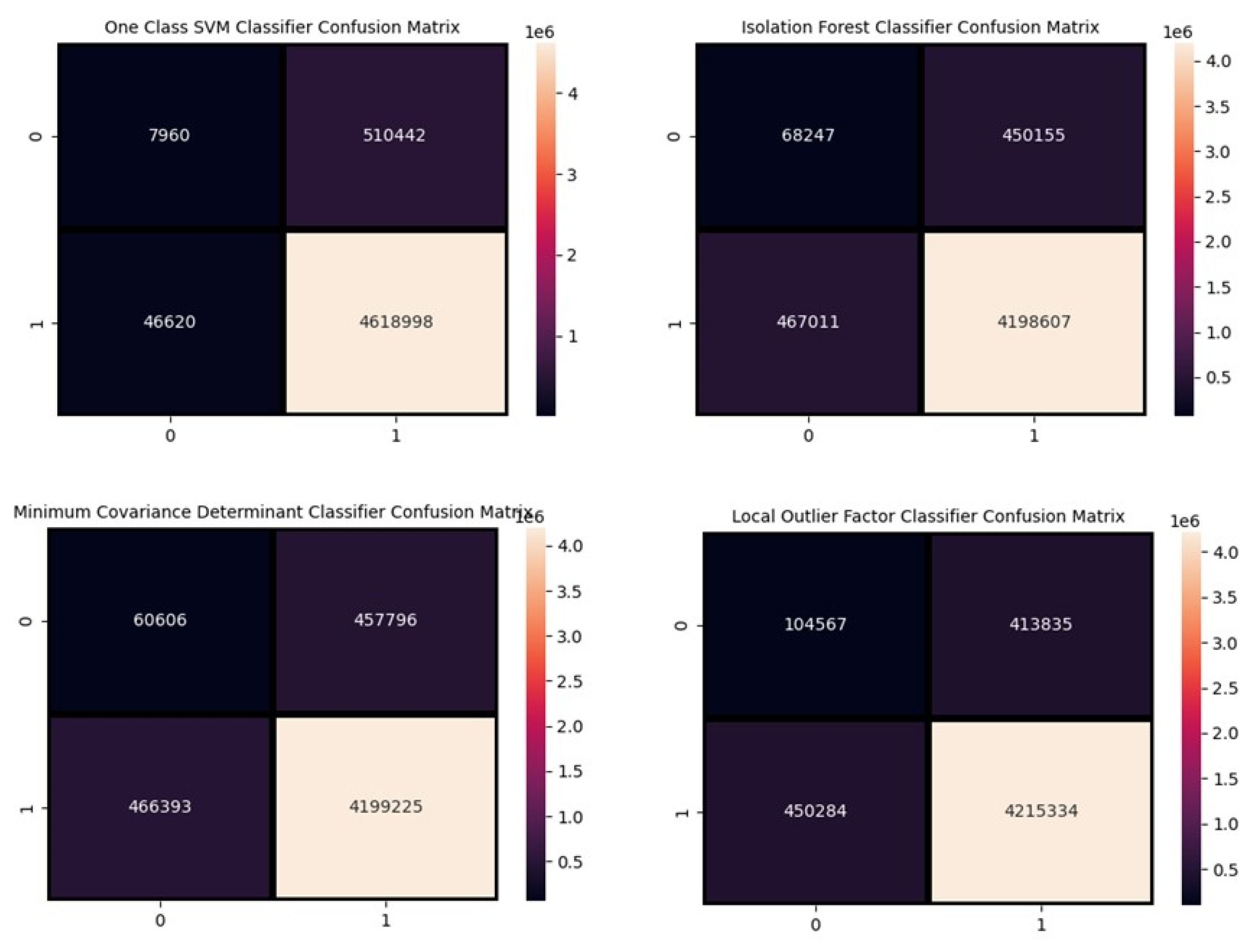
However, to understand the behavior of these algorithms, one can utilize a confusion matrix (see Figure 19, Figure 20 and Figure 21). Here, the number 0 represents the damaged state, while the number 1 represents the healthy state. In this matrix, the horizontal axis signifies the model predictions, and the vertical axis represents the actual data state.

7. Conclusions

The most common metric for assessing algorithm performance in cases of imbalanced data distribution is the F1-Score.

Lack of reliability is closely associated with the customary metrics in machine learning and the intuitions associated with classification accuracy. Typically, practitioners engage with modest datasets where the class distribution tends to be either balanced or nearly balanced. Consequently, they develop an intuition that a lofty accuracy score (or inversely, a low error rate) signifies commendable performance, and values exceeding 90%.

However, achieving an accuracy of 90% or even 99% in an imbalanced classification scenario may not hold substantial significance. This implies that relying on intuitions cultivated for classification accuracy in situations with balanced class distributions can be deceptive. It might lead practitioners to perceive a model’s performance as commendable or even exceptional when, in reality, it falls short of expectations.

Algorithmic approaches to imbalanced classification are considered advanced algorithms, with their ultimate goal being the prediction and identification of the minority class label. This task is more crucial for these algorithms than predicting and identifying the majority class, mainly because the number of unhealthy data instances is much lower than that of healthy data. Separating abnormal (outlier) data becomes challenging, and these algorithms attempt to find specific features among the training data to distinguish and separate the instances.

In the first framework, designed for various coding scenarios, a slight increase in damaged state data has shown improved performance according to the tables in Section 5. Among the algorithms, the Minimum Covariance Determinant algorithm has demonstrated better performance.

In the second framework, facing a vast amount of data, the Isolation Forest and Local Outlier algorithms outperformed the others. Generally, the research results indicate that although the Accuracy Score is high, the F1-Score reveals that the algorithm’s performance is not entirely satisfactory. Various factors may contribute to this, with the primary and most important reason being the lack of specific features and characteristics among the data. It is evident that as the diversity of data increases, feature selection becomes more challenging, potentially leading to suboptimal algorithm performance.

Another reason is the very close proximity of numbers (data points), making the segregation and classification of data difficult. In the second framework, for the initial damaged state where a longer time was spent constructing the bridge and it was subjected to various loads, the data instances of the damaged state became more prominent. It was observed that the algorithm’s performance was significantly better compared with states 2 and 3.

Examining the confusion matrices indicates that while the algorithms performed well in classifying healthy state data, their performance was not satisfactory in identifying and classifying the minority class (damaged state), which is crucial for us. It is evident that the algorithms did not perform well in identifying outlier instances.

Perhaps future optimization of these algorithms could enhance their accuracy and performance.

The majority of methods utilized in previous studies have been tailored for equilibrium states. In these scenarios, the common options often involve either removing data from the analysis or generating artificial data. However, there is potential for the optimization of these algorithms in the future, making them more practical. Furthermore, the exploration and adoption of new algorithms could open up an entirely novel and crucial field. This is particularly significant because, in such approaches, there is no need to alter or delete data, except for cases where transformation is necessary for cleaning and processing. This characteristic serves as a fundamental distinction for algorithms of this nature.

In this article, hardware limitations were present, as the task becomes more demanding with higher amounts of data, necessitating a more powerful system to handle it. Different methods will be employed in the future for damage detection, as this is considered a crucial domain where various algorithms, focusing on classifying imbalanced data, such as Ensemble Algorithms and others, can be utilized.