Composing Diverse Ensembles of Convolutional Neural Networks by Penalization

Abstract

Ensemble-based systems are well known to have the capacity to outperform individual approaches if the ensemble members are sufficiently accurate and diverse. This paper investigates how an efficient ensemble of deep convolutional neural networks (CNNs) can be created by forcing them to adjust their parameters during the training process to increase diversity in their decisions. As a new theoretical approach to reach this aim, we join the member neural architectures via a fully connected layer and insert a new correlation penalty term in the loss function to obstruct their similar operation. With this complementary term, we implement the standard guideline of ensemble creation to increase the members’ diversity for CNNs in a more detailed and flexible way than similar existing techniques. As for applicability, we show that our approach can be efficiently used in various classification tasks. More specifically, we demonstrate its performance in challenging medical image analysis and natural image classification problems. Besides the theoretical considerations and foundations, our experimental findings suggest that the proposed technique is competitive. Namely, on the one hand, the classification rate of the ensemble trained in this way outperformed all the individual accuracies of the state-of-the-art member CNNs according to the standard error functions of these application domains. On the other hand, it is also validated that the ensemble members get more diverse and their accuracies are raised by adding the penalization term. Moreover, we performed a full comparative analysis, including other state-of-the-art ensemble-based approaches recommended for the same classification tasks. This comparative study also confirmed the superiority of our method, as it overcame the current solutions.

1. Introduction

Convolutional neural networks (CNNs) have become top-rated tools in recent years in digital image processing for pattern recognition tasks like detection, localization, segmentation, and classification [1,2,3,4,5,6,7,8,9,10,11]. They have the capability to learn parameters of convolutional filters to extract those significant, higher-order features, which can be used to distinguish images belonging to different classes. The training phase requires thousands of manually labeled images and large-scale computational capacity. The proposed CNNs are sufficiently general to apply them to various classification problems with high accuracy. However, if we intend to improve the classification performance, we may consider the composition of an ensemble from these networks.

Several papers can be found in the literature that consider ensembles of deep learning-based classifiers. Especially, ensemble-based techniques are rather popular to handle regression [12,13], classification [14,15,16], segmentation [17] and metric learning [18] tasks. A pioneer work is [19], where the authors showed that an ensemble of neural networks could achieve higher accuracy than a single one. When we use an ensemble of CNNs or other machine learning-based methods, we have to take into account the following two critical issues: first, how to merge the outputs of the members, and second, how to achieve their diverse behavior to raise accuracy.

There are several ways to aggregate the outputs of the ensemble members. We can calculate, for example, their simple average, arithmetic mean [20] or weighted average. In a weighted aggregation scheme, the weights are usually determined based on the performances of the ensemble members [12,17,21] or by some learning algorithm [14]. We might as well apply voting, where the most common method is the majority-based one [22,23,24]. Moreover, there exist methods which involve also the confidence of the members [25] or assign weights to the voters [26]. In general, the weighting approaches perform better than the unweighted ones because they have extra parameters, which usually lead to a better fit.

Applying a machine learning method for merging the outputs is also quite common, including support vector machine [14], random forest [26], simulated annealing [27], or multi-layer perceptron (MLP) [14]. The main benefit of these learning-based methods is the capability to find the best combination of the members. The cited methods also have a common property: they are used in an offline manner. That is, the members of the ensemble learn their parameters separately before their aggregation. Training the members separately is time consuming and also much harder to make them less correlated, which helps to increase the diversity. On the other hand, we can incorporate the aggregation in the neural architecture to set up an online ensemble with considering fusion layers and concatenation to merge the member outputs. When we use such an ensemble, the members simultaneously can learn their parameters [18,28,29,30], as well. This simultaneous learning shortens the training time, which is a critical issue in deep learning.

Besides the aggregation scheme, another important question is how to achieve large diversity among the members. A corresponding early work [31] recognized that without diversity, the performance of the ensemble becomes limited. There are several methods which could be applied to rise of the diversity of the members. Since offline ensembles are more widespread currently, we start with them first. A possible way is to apply different pre-processing methods [15,23] to make the input more diverse, thus the members also learn different parameters to recognize the various patterns. Others proposed different model architectures [20,25,26] or various kernel sizes and model depth [12]. With the same model architecture but cyclic change of the learning rate, we can also obtain diverse models. This approach is called SnapShot learning [32,33,34] and is able to find different local minima of the loss function that makes the members more diverse. In [22], diversity is raised by splitting an inner layer’s outputs to feed them into other networks. Another possibility is to use custom class weights in the loss function during training [17,23]. With these custom weights, the learning algorithm can be forced to focus on different classes in the training data.

Some of the methods listed so far can be also used online, including, for example, using different pre-processing techniques [29] or different model architectures [35]. However, the simplest and most efficient way for online ensembles is to incorporate the diversity constraints directly into the loss function. The first work that inserted a correlation penalty term in the loss function to force the gradient descent algorithm to learn more diverse ensembles was [13]. This so-called negative correlation learning (NCL) was successfully applied to regression with MLP and used mean square error to calculate the loss. In [28], the same NCL technique was considered for CNN in crowd counting, age estimation, personality analysis and single-image super-resolution tasks. An inner layer of the CNN was split, and the separated outputs were fed into three “sub-networks”. The NCL method was combined with AdaBoost for MLPs in [36] to solve classification problems. In [18], a custom loss function was presented to achieve a diverse and less correlated embedding for image metric learning. The cosine similarity also can be used as a penalty term to raise diversity [29]. The cooperative ensemble was also investigated here by KL-divergence and was combined with differently pre-processed images and network dropout to make it more diverse.

In the current work, we propose an online ensemble technique for image classification. As our main contribution, we introduce a new, more refined penalty term than NCL for a loss function dedicated to classification purposes. Namely, we use the Pearson-correlation penalty term instead of the simple one of NCL, which is able to simultaneously support the correlation for correct decisions, while supporting uncorrelated behaviors of the members for false decisions. On the other hand, instead of using MSE like in the former works related to NCL, we use categorical cross entropy, which is currently a better accepted loss function for classification scenarios. Nevertheless, notice that though we use our penalty term with a cross-entropy loss, it can be applied to any other one in the same way. Finally, as a supplementary step, we also adopt the strategy to include different types of member architectures.

In our former work [35], we combined different individual CNN architectures that have already proven their efficiencies in pattern recognition scenarios. We elaborated on an ensemble-based framework, which can be successfully applied to improve the accuracy of individual CNNs if the expansion of the training image set is not possible. We trained the four CNN architectures GoogLeNet [37], AlexNet [38], ResNet [39] and VGGNet [40] and aggregated their outputs. We showed how to train different CNNs in parallel and fuse their outputs based on specific mathematical and statistical models to improve the final classification accuracy. This solution can be considered a rather loosely connected ensemble-based system since the members are trained completely independently from each other.

As an improvement, we proposed the fusion of the CNNs at the architecture level in a later work. Thus, we composed a much more complex, combined super-network and trained the involved members as a whole [41]. More specifically, we interconnected the members with inserting a joint fully connected layer followed by the classic softmax/classification ones for the final prediction. In this way, we created a single network architecture from the member CNNs, which can be trained by backpropagation in a standard way.

In this work, we improve the final classification accuracy of the composed ensemble further by forcing the members to adjust their parameters during backpropagation to increase the diversity in their decisions. More specifically, we join the member CNNs via a fully connected layer and introduce a new term in the loss function as a correlation penalty, which rises when the individual neural networks misclassify at the same time. With this approach, we implement the traditional common guideline to increase the diverse behaviors of the members also for ensembles of CNNs. As an additional theoretical contribution, we properly determine the derivative of the introduced loss function to be able to implement the backpropagation procedure efficiently. The benefits of our general method is demonstrated on four classification problems related to natural images and medical ones. Besides the theoretical considerations and foundations, our experimental results suggest that the proposed approach is a highly competitive one.

The rest of the paper is organized as follows. In Section 2, we introduce our methodology for creating an ensemble of CNNs. We also present how a term penalizing the correlation of the member CNNs on the false decisions is added to the loss function. To highlight our main contribution, we also give a formal derivation to prove the positive effects of our penalty term for the ensemble diversity. We also provide the partial derivatives of the penalty term in a closed form to be able to integrate it seamlessly to the backpropagation process to adjust the corresponding weights in the joint network. Section 3 is dedicated to our experimental results in classification tasks related to the automatic recognition of skin cancer and the severity of diabetic retinopathy (DR) from several aspects and evaluating our method on well-known natural image data sets, as well. We also compare our method with some state-of-the-art ensemble-based techniques suggested for the same type of classification tasks. Finally, some conclusions are drawn in Section 4.

2. Learning Methodology

Recently, in the field of natural image classification, several CNN architectures have been released, like GoogLeNet [37], AlexNet [38], ResNet [39], VGGNet [40], DensNet [42], and MobileNet [43], besides others. Some of these architectures are available as pre-trained models initially trained on approximately 1.28 million natural images from the data set ImageNet [44]. Thus, as a transfer learning approach [45], we can use the weights and biases from these pre-trained models. That is, if we fine-tune all the layers of these models by going on with the backpropagation using our data, they can be applied to our specific classification task, as well. On the other hand, if we have sufficiently many annotated images to train from scratch, we can initialize the parameters of the CNNs randomly.

This study considers both randomly initialized and pre-trained networks also designed for deep learning purposes. We fuse these networks during the creation of the ensemble and produce a directed acyclic graph, where layers can have inputs from multiple ones. In practice, we combine the outputs of the members using a concatenation layer, which is a dense one. The general aim of an ensemble system is to benefit from the members’ strengths while overcoming their weaknesses. Unfortunately, some critical problems may arise during the combination of members’ outputs. The worst situation is when more than one member predicts the same wrong class label for the same input because member classifiers are trained on the same data set to minimize the same loss function. To improve the final accuracy in image classification, we elaborated a method that ensures that the outputs of the members will be combined efficiently, and their diversity (regarding the wrongly classified cases) is also aimed to be increased.

As a realization of this idea, we create an ensemble of some well-known CNNs to increase classification accuracy via a new network architecture. The interconnection of the member CNNs is solved with an additional fully connected (FC) layer inserted after the last FC layers of the original CNNs. We initialize/load the weights of this layer and extend the categorical/binary cross-entropy loss function with an extra term, which can be considered a correlation penalty to enforce more diverse behavior of the participating CNNs. In this study, cross entropy is considered, as it has been widely used as a single loss function and also to construct a hybrid loss function particularly for object classification [46,47,48,49]. However, our approach also supports any other loss functions. As the main contribution of this work, we implement the common guideline with adding a new term to diversify the members for the ensemble of CNNs. In this way, the constructed ensemble architecture can train the weights of the combination of two or more networks according to their diversity.

2.1. The Fusion of the Member Networks

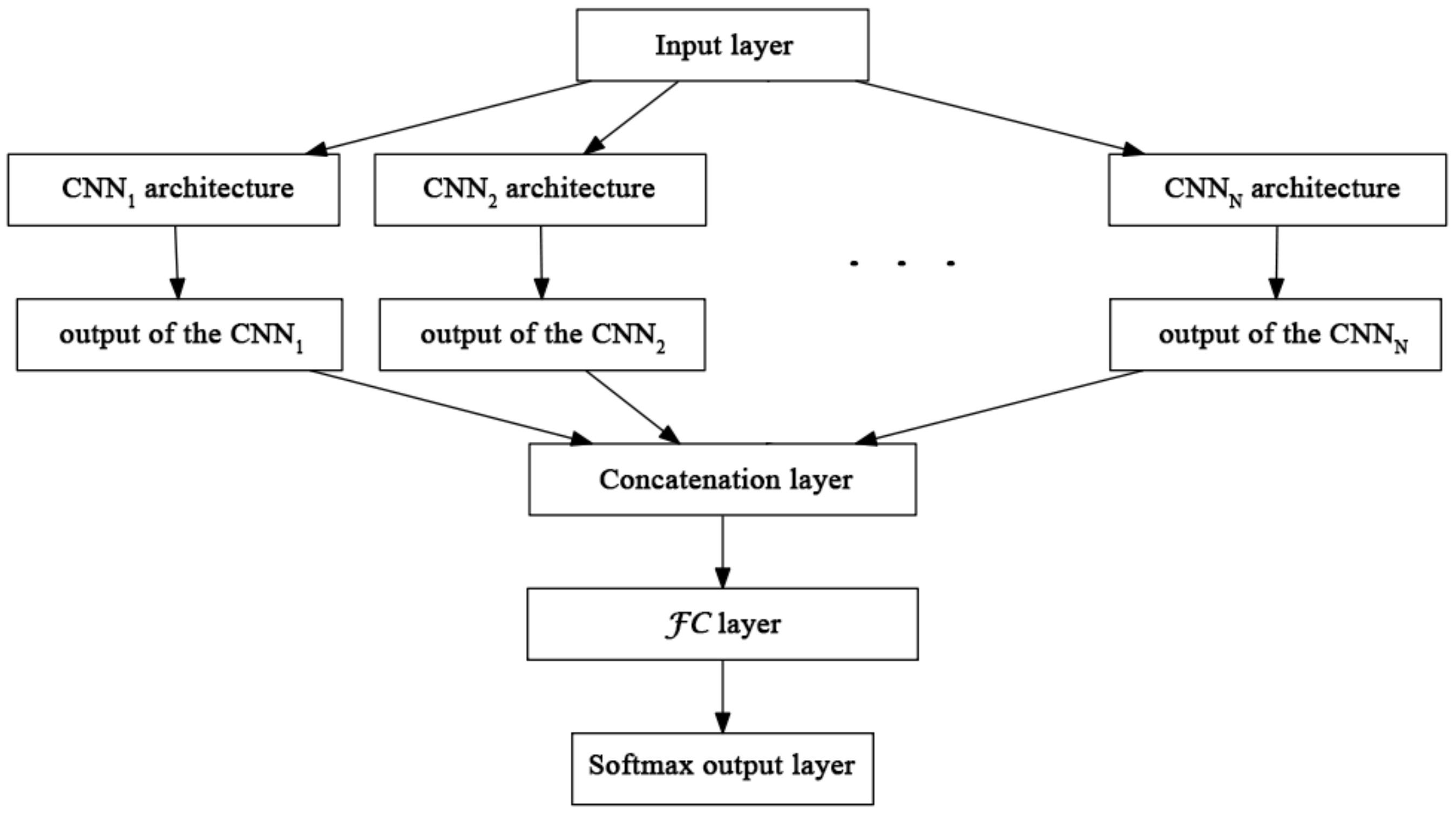
This section presents how we produce a single neural network architecture as an ensemble of N member CNNs. For this aim, we remove their softmax output layers. To prepare the member CNNs for the current classification task, we replace their last FC layers with other ones, whose output sizes are set to the required number of classes. We connect the CNNs via these FC layers with a concatenation one and combine them with an additional fully connected layer $\mathcal{FC}$. The input of $\mathcal{FC}$ is a concatenated vector built from the outputs of the member CNNs, and the $\mathcal{FC}$ layer creates its output as a weighted combination of these values, as it can be seen in Figure 1.

To give the proper formal description of our approach, let us denote the training set by

$$\{x^{\left(n\right)},n=1,\dots ,M\},$$

where the given true labels are

$$\{d^{\left(n\right)},n=1,\dots ,M\}.$$

Here, M denotes the number of samples in the training set, while L is the number of classes (typically $L\ll M$) and the labels $d^{\left(n\right)}$ are L-dimensional one-hot vectors. For the n-th training sample, let $F_i^{\left(n\right)}$ be the output of the softmax layer of the i-th CNN ($i=1,\dots ,N$), which is a probability distribution vector of dimension L, where the i-th coordinate gives the probability that the given training sample corresponds to the i-th class. As an ensemble of the member networks, the $\mathcal{FC}$ layer computes the linear combination

$${\tilde{F}}_{ens}^{\left(n\right)}=\sum _{i=1}^N{A}_i{F}_i^{\left(n\right)},$$

where the coefficients $A_i$ are initialized as $L\times L$ matrices close to a diagonal one with equal weights in their diagonals and small ($\epsilon \approx 0$) values outside the diagonal:

$$A_i=\left(\begin{array}{cccc}1/N& \epsilon & \cdots & \epsilon \\ \epsilon & 1/N& \cdots & \epsilon \\ ⋮& & & \\ \epsilon & \epsilon & \cdots & 1/N\end{array}\right).$$

(1)

Practically, that means that we take approximately the arithmetical mean of the outputs of the members initially. However, the weights of these vectors are trainable parameters of the network, so these parameters are also changed during the backpropagation steps of the training phase. To follow the common principles, at the end of this ensemble, we also insert a softmax layer to convert the vector ${\tilde{F}}_{ens}^{\left(n\right)}$ to a probability distribution $F_{ens}^{\left(n\right)}$.

2.2. The Loss Function

To increase the diversity of the member networks and avoid the jointly misclassified items, we introduce a new loss function to achieve higher final classification accuracy. We supply the cross-entropy loss function with our proposed penalty term, penalizing when the member networks work similarly wrong and simultaneously supporting correct decisions.

For this aim, we define the penalty function E with the help of the Pearson correlation coefficient. If $X=(X_1,\dots ,X_K)$ and $Y=(Y_1,\dots ,Y_K)$ are K-dimensional vectors, then their Pearson correlation coefficient can be calculated as

$$\begin{array}{cc}\hfill \varrho (X,Y)& =\frac{1}{K-1}\sum _{i=1}^K\left(\frac{X_i-\overline{X}}{{\sigma }_X}\right)\left(\frac{Y_i-\overline{Y}}{{\sigma }_Y}\right)\hfill \\ & =\frac{{\displaystyle \sum _{i=1}^K}(X_i-\overline{X})(Y_i-\overline{Y})}{\sqrt{{\displaystyle \sum _{i=1}^K}{(X_i-\overline{X})}^2{\displaystyle \sum _{i=1}^K}{(Y_i-\overline{Y})}^2}},\hfill \end{array}$$

where $\overline{X}$ and $\overline{Y}$ are the means of X and Y, while ${\sigma }_X$ and ${\sigma }_Y$ denote the corresponding standard deviations, respectively.

Using the notation introduced in Section 2.1, let $C^{\left(n\right)}$ be the correlation matrix of the vectors $F_1^{\left(n\right)}$, $F_2^{\left(n\right)},\dots ,F_N^{\left(n\right)}$ and $-d^{\left(n\right)}$:

$$C^{\left(n\right)}=\left(\begin{array}{cccc}\varrho (F_1^{\left(n\right)},F_1^{\left(n\right)})& \dots & \varrho (F_1^{\left(n\right)},F_N^{\left(n\right)})& -\varrho (F_1^{\left(n\right)},d^{\left(n\right)})\\ \varrho (F_2^{\left(n\right)},F_1^{\left(n\right)})& \cdots & \varrho (F_2^{\left(n\right)},F_N^{\left(n\right)})& -\varrho (F_2^{\left(n\right)},d^{\left(n\right)})\\ ⋮& \\ \varrho (F_N^{\left(n\right)},F_1^{\left(n\right)})& \cdots & \varrho (F_N^{\left(n\right)},F_N^{\left(n\right)})& -\varrho (F_N^{\left(n\right)},d^{\left(n\right)})\\ -\varrho (d^{\left(n\right)},F_1^{\left(n\right)})& \cdots & -\varrho (d^{\left(n\right)},F_N^{\left(n\right)})& \varrho (d^{\left(n\right)},d^{\left(n\right)})\end{array}\right),$$

which is a symmetric one of dimension $(N+1)\times (N+1)$.

Then, the penalty term E is defined as

$$E=\frac{1}{M}\sum _{n=1}^M\left[\sum _{i=1}^N\sum _{j=i}^N{C}_{ij}^{\left(n\right)}+N\sum _{i=1}^{N+1}{C}_{i,N+1}^{\left(n\right)}\right].$$

(2)

That is, we consider the $N\times N$ upper-left part of the matrix $C^{\left(n\right)}$, take the sum of the entries in the upper triangular part of this latter matrix, and add the sum of elements in the last column of $C^{\left(n\right)}$ with weight N. Finally, we calculate the mean of the $C^{\left(n\right)}$ values for $n=1,\cdots ,M$. Note that the values standing in the main diagonal of $C^{\left(n\right)}$ are equal to 1, which means a constant term in the penalty function.

As a next step, we give a formal proof that the penalty term E introduced in (2) owns the properties to improve the ensemble performance.

Proposition 1.

Including the penalty term (2) provides a loss function, having increasing values according to the order of the following cases:

• All the experts (member networks) classify the n-th training sample correctly;
• Some of the experts do not assign the n-th training sample to the true class, but their outputs are different classes;
• Some of the experts classify the n-th training sample in the same false class;
• All experts assign the n-th training sample to false classes, but these classes differ;
• All experts assign the n-th training sample to the same false class.

Proof. 

See Appendix A. □

We use the penalty term E with a $\lambda \ge 0$ weight in the final loss function:

$${\mathcal{L}}_f=\mathcal{L}+\lambda E,$$

(3)

where $\mathcal{L}$ is the original cross-entropy loss function. The role of $\lambda$ is to control the effect of the penalty term: increasing its value means that we try to increase the diversity of the member networks. Naturally, a too-high $\lambda$ value has a negative effect, because in this case, the diversity operates against the accuracy.

Finally, to help the implementation of the backpropagation process, we describe the partial derivative of the penalty term with respect to the coordinates of $F_k^{\left(n\right)}$ for $k=1,\dots ,N$. Denoting by $F_{k,m}^{\left(n\right)}$ the m-th coordinate of $F_k^{\left(n\right)}$, we obtain that

$$\frac{\partial E}{\partial F_{k,m}^{\left(n\right)}}=\frac{1}{M}\sum _{n=1}^M\left[\sum _{\begin{array}{c}j=1\\ j\ne k\end{array}}^N\frac{\partial C_{kj}^{\left(n\right)}}{\partial F_{k,m}^{\left(n\right)}}+N\frac{\partial C_{k,N+1}^{\left(n\right)}}{\partial F_{k,m}^{\left(n\right)}}\right],$$

where the partial derivatives of the correlation coefficients can be calculated as

$$\frac{\partial \varrho (X,Y)}{\partial X_m}=\frac{(Y_m-\overline{Y})-\frac{{\displaystyle \sum _{i=1}^K}(X_i-\overline{X})(Y_i-\overline{Y})}{{\displaystyle \sum _{i=1}^K}{(X_i-\overline{X})}^2}(X_m-\overline{X})}{\sqrt{{\displaystyle \sum _{i=1}^K}{(X_i-\overline{X})}^2{\displaystyle \sum _{i=1}^K}{(Y_i-\overline{Y})}^2}}.$$

3. Application to Image Classification Problems

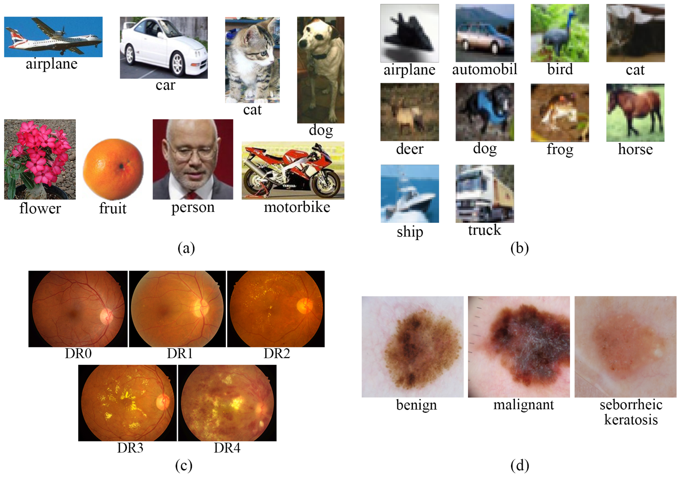
For the experimental evaluation of our approach, we used some different well-known CNNs and composed their ensembles to show the usability of our proposed solution. We also demonstrate the positive effects of our penalization term on the classification accuracy by reducing the correlation of the members’ outputs. We involved four different image sets (see Figure 2) for the comprehensive evaluation and used them to train the models and evaluate their performances.

3.1. Data Sets and Preparations

To show the improvement obtained by using the proposed penalty term, we evaluated our approach on the natural image sets ISINI [50], and CIFAR-10 [51], which are the commonly used ones in the related literature. Moreover, as a special field currently investigated by us, we also involved the skin lesion data set [52] and the DR ones [53,54,55] to see the possible classification accuracy gain provided by greater diversity.

3.1.1. ISINI Image Set

The ISINI data set is published by Prasun et al. in [50], and it contains 6899 images classified into eight classes: airplane, car, cat, dog, flower, fruit, motorbike, and person (see sample images in Figure 2a). All the classes contain almost the same number of items (727, 968, 885, 702, 843, 1000, 788, and 986 samples from the eight classes, respectively), which supports the efficient training of the CNNs for each class. The images have different resolutions varying from $43\times 114$ to $2737\times 2229$ pixels, hence we resized them to the same size of $227\times 227$ pixels to overcome these differences. To train the neural networks, we split the set into training (5519) and test (1380) parts with keeping up the original ratio among the classes.

3.1.2. CIFAR-10 Image Set

The CIFAR-10 natural image set is published in [51] by Krizhevsky et al. in 2009, and it is one of the most commonly used data sets for the evaluation of different CNNs. The CIFAR-10 data set consists of 60,000 $32\times 32$ color images in 10 classes, with 6000 images per class. The low resolution of these images can also be observed in Figure 2b. In total, 50,000 training and 10,000 test images are provided, and we also used this original partitioning. The class labels are airplane, automobile, bird, cat, deer, dog, frog, horse, ship, and truck. As for this data set, the original image resolution was kept and instead of resizing the images, we replaced the input layers of the architecture with the appropriate ones.

3.1.3. DR Image Set

To prove the usability of the proposed ensemble model and the penalty term, we considered a DR image classification task to check whether the performance can be increased in this application as well. We merged the data sets Kaggle DR [54], Messidor [55], and the Indian Diabetic Retinopathy Image Dataset (IDRiD) [53] into a single one and split it into a training and test part. Each of the three data sets contains digital retinal images of different resolutions (400 × 315, 1440 × 960, 2240 × 1488, 2304 × 1536, 4288 × 2848, and 5184 × 3456 pixels) and different fields of view. Each image is categorized according to the severity of DR (5 classes), which means the images are labeled as no (DR0), mild (DR1), moderate (DR2), severe (DR3), and proliferative DR (DR4). Some sample images from these classes can be seen in Figure 2c. The DR grading score is provided for 18,127/4529 training/test images, among which 9975/2493 are categorized as DR0, 2085/520 as DR1, 4537/1134 as DR2, 757/189 as DR3, and 773/193 as DR4.

3.1.4. ISIC Image Set

To have an even more reliable evaluation for the clinical domain as our primary target, we considered a skin lesion image set as well. The ISIC image set was published by Codella et al. in [52], which has a training part containing 2000 images (samples can be seen in Figure 2d) with manual annotations regarding three different classes in the following compounds: 1372 images with nevus, 254 with seborrheic keratosis, and 374 ones with malignant skin tumors. The images from this training set were used to fine tune the constructed ensemble network, and the evaluation was performed on the test set. The test set consists of 393 nevus, 90 melanoma, and 117 seborrheic keratosis images, respectively.

3.1.5. Image Augmentation

Regarding the ISINI, ISIC, and DR data sets, the volumes of images in certain classes are not sufficiently large to train CNNs and their ensembles [44] without overfitting. To overcome this issue, we followed the common recommendation regarding the augmentation of the training data set. There are several possibilities for data augmentation, like image shearing with randomly selected angle (max: ${20}^{\circ }$) in the counter-clockwise direction, random zooming from range [$0.8$–$1.2$], flipping horizontally, and rotating with different random angles. Using such transformations, we made some minor modifications to the training images, which helps to avoid the overfitting of the models.

3.2. Convolution Neural Networks and Their Ensemble

As for the design of the ensemble network architecture, our main motivation was to use reliable classifiers as backbone architectures and compare the aggregated results to their original individual accuracies. In the field of natural image classification, several CNN architectures have been released, like AlexNet, VGG16, GoogLeNet Inception-v3, MobileNetV2 and ResNet50, which were reported to show solid performances.

AlexNet consists of five convolutional layers some of which are followed by max-pooling layers and three FC layers with a final softmax one. The FC layer before the last one has 4096 neurons, which means that it extracts the same number of features from each input image and uses them to predict the class label at the last FC layer. VGGNet has a depth between 16 and 19 layers and consists of small-sized convolutional filters. In VGG16, we used the configuration consisting of 13 convolutional layers with filters of size $3\times 3$ pixels. A stack of convolutional layers is followed by three FC layers, where the last one has the same number of neurons as the class labels required. For the medical image classification tasks, some deeper and newer architectures are also involved in our ensembles, such as MobileNetV2, ResNet50, and GoogLeNet Inception-v3. The MobileNetV2 is based on an inverted residual structure, and its intermediate expansion layer uses lightweight convolutions to extract important features of the image. This CNN contains initial fully convolution layer with 32 filters, followed by 19 residual bottleneck layers. ResNet50 has 48 convolution layers along with 1 max-pool layer and 1 average-pool layer. This network architecture can handle the problem of vanishing/exploding gradients with the benefit of shortcut identity mapping, which is known as the deep residual learning technique. Finally, we considered GoogLeNet Inception-v3 for our ensemble regarding the dermatology image classification task, as GoogLeNet is reported to show a solid performance in skin lesion classification [56], as well.

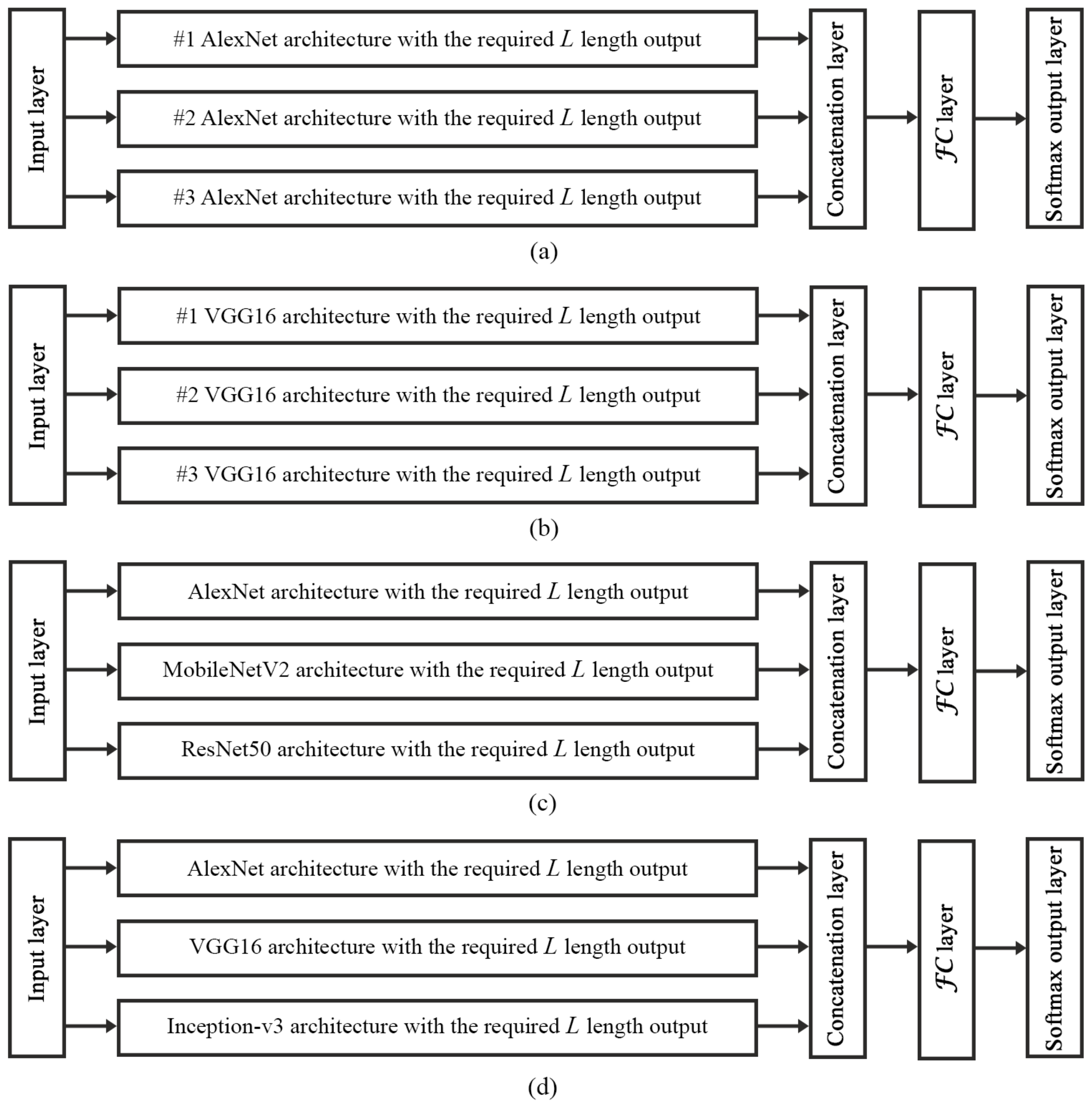
To create an ensemble architecture from these CNNs, we prepared the members for the given image classification task. Thus, we replaced their last FC layers with other ones having the length of the number of classes, and connected these FC layers with an additional fully connected layer $\mathcal{FC}$ as described in Section 2.1. Altogether, we composed four different ensemble networks to make an exhaustive evaluation and show that the proposed methodology for connecting CNNs and training them simultaneously by using the $\lambda E$ penalty term has a capability to improve the accuracy with increasing the diversity between the members. There are two types of ensembles. The first one contains the same architecture multiple times to demonstrate how the penalty term makes the similar architectures more diverse (see Figure 3a,b). In the second one, we combine some different CNN models to make an initially diverse ensemble architecture (see Figure 3c,d) and to train them simultaneously. Our aim was to show that if we considered the state-of-the-art models and fused them, we can outperform their individual accuracies. The ensemble network is optimized on different data sets with applying the penalized loss function with different $\lambda$ values.

3.3. Experimental Results

We used the four data sets introduced in Section 3.1.1–Section 3.1.4 and four different setups of the ensembles of the CNNs to validate the benefit of the proposed penalty term regarding the final accuracy. Moreover, to exclude any random noise and confirm the achieved results, we repeated each experiment five times and calculated the mean accuracies and standard deviations.

In the first scenario, to measure the effects of the penalization term on the ensemble architecture during the training stage, we considered the simplest ensemble to avoid any unexpected effects derived from the complexity of the member CNNs. Accordingly, we included only the AlexNet network three times to compose the ensemble, as it can be seen in Figure 3a. To ensure a reliable comparison, we evaluated the classification performance of a single AlexNet and its ensemble with and without ($\lambda =0$) using the proposed penalization term. Moreover, we applied different $\lambda$ values in (3) to show how the members become more diverse as $\lambda$ increases.

To have also a comparison with other approaches, we considered some frequently applied state-of-the-art ensemble methods to show the superiority of the proposed combination framework, where the members can be trained simultaneously. As we described in the introduction, there are some well-known aggregation methods, which can be applied successfully to increase the global accuracy. One of them is simple majority voting (SMV) when we check the outputs of the members and select the label supported by the largest number of votes as in [22,23]. SMV could provide false labels when none of the members finds the correct class or when more members predict the same wrong class than the correct one. If we have some information about the reliability or the individual accuracies of the members, we can exploit this knowledge for weighting the votes accordingly to realize weighted majority voting (WMV) as in [26]. As a last method for comparison, we include the simple averaging (AVE) when the member outputs are merged by calculating the arithmetic mean of their softmax outputs as it is proposed in [20].

The details of these evaluations can be seen in

Table 1. Classification accuracy of different setups of AlexNet on the ISINI set.

CNN Architecture	Value of $\mathit{\lambda }$	Accuracy	Total # of Missed Images	Double Missed	Triple Missed
single AlexNet	-	0.9328 ± 0.0029	92.6 ± 4.04	-	-
SMV	-	0.9465 ± 0.0047	74 ± 6.53	51.0 ± 4.12	27.8 ± 3.50
WMV	-	0.9462 ± 0.0041	74 ± 5.67	51.0 ± 4.12	27.8 ± 3.50
AVE	-	0.9504 ± 0.0021	68 ± 2.96	51.0 ± 4.12	27.8 ± 3.50
AlexNet multi	0	0.9543 ± 0.0013	63 ± 1.73	50.4 ± 3.42	27.6 ± 3.51
AlexNet multi	0.5	0.9636 ± 0.0021	50 ± 2.94	36.2 ± 3.99	24.0 ± 3.67
AlexNet multi	1	0.9650 ± 0.0018	48 ± 2.49	32.0 ± 4.99	25.0 ± 4.30
AlexNet multi	5	0.9617 ± 0.0013	52 ± 1.78	31.4 ± 2.82	24.4 ± 2.96

, where AlexNet multi stands for the ensemble architecture trained by different strength penalization $\lambda$ terms.

Table 1 shows the accuracies and the number of misclassified images regarding the single AlexNet and its different ensembles with and without ($\lambda =0$) applying the penalization term. If we check the accuracy values, a $3\%$ improvement can be observed over all the investigated state-of-the-art combination methods and the individual member accuracies. Our aim was to improve the classification accuracy and make the members more diverse to reduce the chance of simultaneous mistakes. To show how the proposed penalization term reduced the number of simultaneously misclassified items, we considered the outputs of the members and evaluated their individual accuracies with increasing the value of $\lambda$, as well. Moreover, we checked how many images are classified wrongly by at least two members. Accordingly, the last two columns of Table 1 show the average number of images which were classified wrongly by two members (double missed) and three members (triple missed). We can see that the number of jointly missed images decreases when $\lambda$ increases, and in this way, the proposed penalty term E is applied during training. So it can be used efficiently to reduce the incidence of joint mistakes of the members. Notice that if we set $\lambda$ to a higher value, the penalty term becomes stronger, resulting in lower classification accuracy, as the optimization process focuses better on the more diverse members.

To further check the usability and efficiency of the proposed penalty term, we trained and evaluated AlexNet and its ensemble on the CIFAR-10 image set (see

Table 2. Classification accuracy of different setups of AlexNet on the CIFAR-10 set.

CNN Architecture	Value of $\mathit{\lambda }$	Accuracy	Total # of Missed Images	Double Missed	Triple Missed
single AlexNet	-	0.6431 ± 0.0056	3569 ± 56	-	-
SMV	-	0.6308 ± 0.0024	3692 ± 25	3797 ± 362	2692 ± 130
WMV	-	0.6258 ± 0.0044	3741 ± 44	3797 ± 362	2692 ± 130
AVE	-	0.6554 ± 0.0079	3446 ± 79	3797 ± 362	2692 ± 130
AlexNet multi	0	0.6471 ± 0.0031	3529 ± 31	3093 ± 248	2741 ± 79
AlexNet multi	0.5	0.6656 ± 0.0059	3343 ± 59	2124 ± 165	2290 ± 48
AlexNet multi	1	0.6683 ± 0.0035	3316 ± 35	2077 ± 254	2294 ± 45
AlexNet multi	5	0.6646 ± 0.0042	3354 ± 42	2130 ± 261	2295 ± 119

for the results). In this scenario, we can observe a slight improvement considering the accuracy ($2.5\%$), which means that more 253 images were classified correctly. Even more importantly, the double/triple misses dropped remarkably, showing that higher diversity is reached. Raising $\lambda$ above a given point could have harmful effect on the global classification accuracy just in our previous setup and all the further experiments.

For the sake of completeness, VGG16 is also involved in the same type of evaluation using the CIFAR-10 data set. So, we trained the single VGG16, composed its ensemble in the same way as AlexNet and measured the classification accuracies with and without applying the proposed penalization term. The results enclosed in

Table 3. Classification accuracy of different setups of VGG16 on the CIFAR-10 set.

CNN Architecture	Value of $\mathit{\lambda }$	Accuracy	Total # of Missed Images	Double Missed	Triple Missed
single VGG16	-	0.8051 ± 0.0016	1949 ± 16	-	-
SMV	-	0.7800 ± 0.0243	2199 ± 243	2036 ± 274	660 ± 48
WMV	-	0.8197 ± 0.0111	1802 ± 111	2 036 ± 274	660 ± 48
AVE	-	0.8331 ± 0.0060	1668 ± 60	2036 ± 274	660 ± 48
VGG16 multi	0	0.8743 ± 0.0013	1256 ± 13	1537 ± 318	661 ± 49
VGG16 multi	0.5	0.8923 ± 0.0024	1077 ± 25	812 ± 31	540 ± 13
VGG16 multi	1	0.8931 ± 0.0018	1068 ± 18	818 ± 30	526 ± 30
VGG16 multi	5	0.8892 ± 0.0027	1108 ± 27	908 ± 44	545 ± 29

show a $7\%$ rise in classification accuracy when we compose an ensemble using more VGG16 networks by only concatenating and training them together instead of combining their outputs after a separate training. The performance is increased with an additional $2\%$ when the proposed penalization term is applied. Moreover, the number of jointly missed images is reduced dramatically.

To demonstrate the efficiency of the proposed combination and the penalty term also for medical image classification tasks, we considered an ensemble network composed from AlexNet, MobileNetV2, and ResNet50 as it can be seen in Figure 3c. As a first step, we trained the members separately as individual architectures and calculated their accuracies. Then, we took their outputs and combined them using SMV, WMV, and AVE, respectively. Finally, we connected these member CNNs to form a single architecture and trained them simultaneously using the proposed concatenation layer and the penalty term with different $\lambda$ values. As we can see in

Table 4. Classification accuracy of the ensemble of CNNs on the DR data set.

CNN Architecture	Value of $\mathit{\lambda }$	Accuracy	Total # of Missed Images	Double Missed	Triple Missed
AlexNet	-	0.5760 ± 0.0035	1920 ± 16	-	-
MobileNetV2	-	0.6114 ± 0.0101	1760 ± 46	-	-
ResNet50	-	0.6515 ± 0.0193	1578 ± 87	-	-
SMV	-	0.6250 ± 0.0163	1698 ± 73	600 ± 50	1110 ± 111
WMV	-	0.6384 ± 0.0182	1637 ± 82	600 ± 50	1110 ± 111
AVE	-	0.6462 ± 0.0182	1602 ± 82	600 ± 50	1110 ± 111
CNN ensemble	0	0.6584 ± 0.0170	1547 ± 77	580 ± 152	1136 ± 86
CNN ensemble	0.5	0.6707 ± 0.0081	1491 ± 36	460 ± 140	883 ± 21
CNN ensemble	1	0.6662 ± 0.0034	1511 ± 15	651 ± 128	866 ± 27
CNN ensemble	5	0.6599 ± 0.0099	1540 ± 45	742 ± 224	913 ± 122

, the model composed by the proposed combination framework after training with the penalty term E reached 2–$5\%$ higher accuracy than SMV/WMV/AVE, and the number of the simultaneously misclassified fundus images decreased as well.

As our final use case, we checked the usability and effectiveness of our proposed combination technique in skin lesion classification. We have already made substantial efforts in this field to improve classification accuracy, e.g., in an ensemble-based manner. In [35], we considered four different CNN architectures, and after training them in parallel, we fused their outputs using statistical models. In [41], we interconnected the CNNs by inserting a joint fully connected layer and composed a super-network in which all the members are trained together. Now, we use the same CNNs and data set [52] and show how the proposed penalization term can help the members to become more diverse to make the ensemble-based system reach higher classification accuracy.

At this point, we have composed an ensemble-based system (see Figure 3d) from AlexNet, VGG16 and GoogLeNet Inception-v3 as we described in Section 2.1 and Section 3.2. The classification performances of the individual models and their ensembles using different $\lambda$ values can be seen in

Table 5. Classification accuracy of the ensemble of CNNs on the ISIC data set.

CNN Architecture	Value of $\mathit{\lambda }$	Accuracy	Total # of Missed Images	Double Missed	Triple Missed
AlexNet	-	0.6858 ± 0.0011	188 ± 1	-	-
VGG16	-	0.7033 ± 0.0014	178 ± 1	-	-
Inception-v3	-	0.7099 ± 0.0016	174 ± 1	-	-
CNN ensemble	0	0.7011 ± 0.0239	179 ± 14	99 ± 30	106 ± 7
CNN ensemble	0.5	0.7294 ± 0.0178	162 ± 11	102 ± 29	94 ± 13
CNN ensemble	1	0.7355 ± 0.0111	158 ± 6	150 ± 31	57 ± 37
CNN ensemble	5	0.7011 ± 0.0267	179 ± 16	177 ± 25	39 ± 8

, where $\lambda =0$ can be considered the result of a previous approach published in [41].

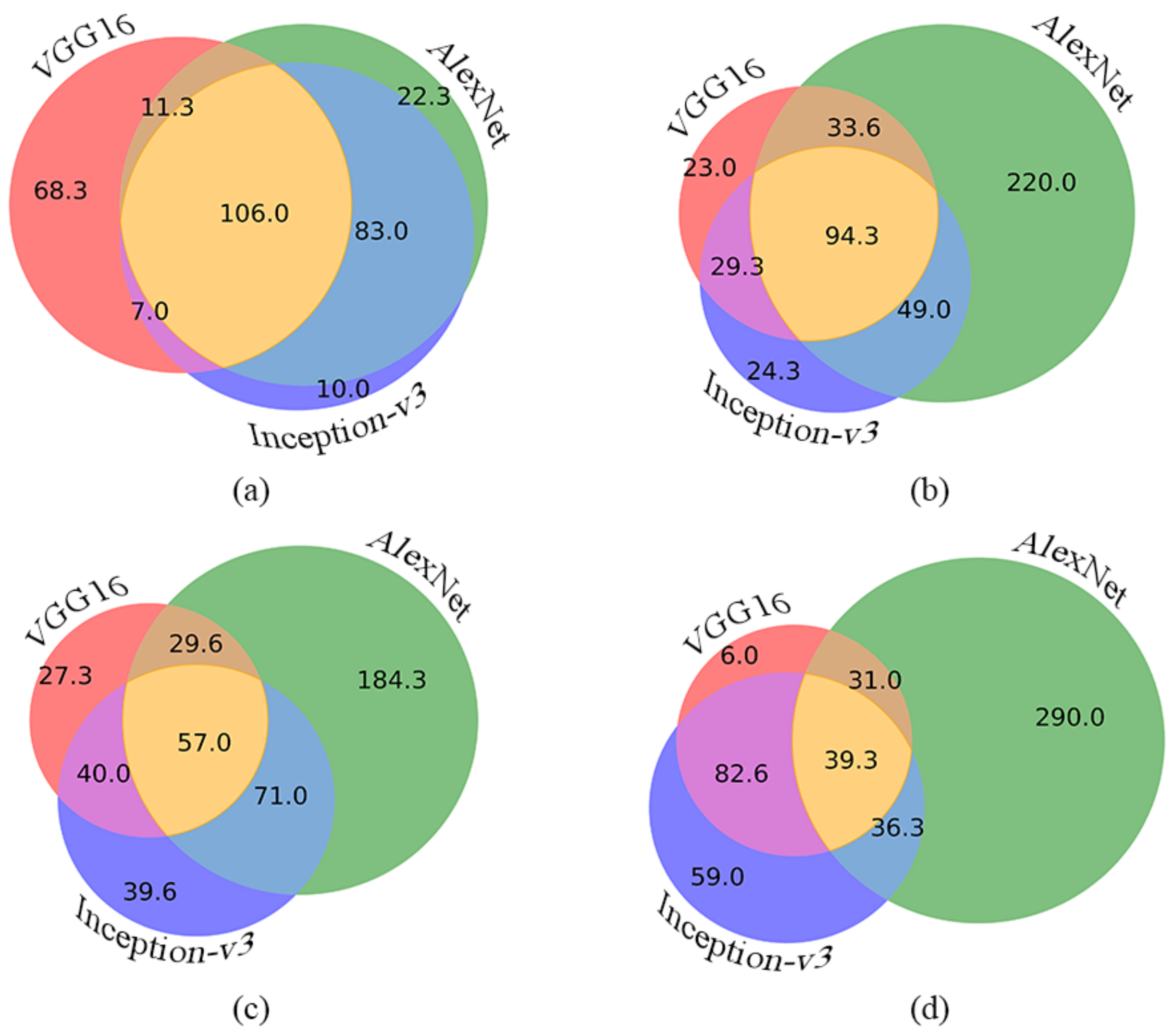
We can see a more than $3\%$ improvement in classification regarding our previous ensemble-based method and a remarkable growth in diversity based on the drops of the double/triple misses at $\lambda =1$. In one of the five runs with $\lambda =1$, the ensemble network reached its best performance when it missed only 151 images, so its accuracy was $74.8\%$. For a better interpretation, we also give a visual representation on how the ratios of the single, double, and triple misses change for $\lambda =0$, $\lambda =0.5$, $\lambda =1$, and $\lambda =5$ (see Figure 4a,b,c,d, respectively). In these charts, each disc contains the average number of the missed images by the given member. The intersecting parts contain the average numbers of the double and triple missed images.

To make our comparative study more comprehensive, we also applied the evaluation protocol of the ISBI 2017 challenge [52]. Namely, we converted the originally three-classes task to three binary classification problems using the one-vs-all approach. Then, the performance was evaluated as the average of the three binary classification accuracies. In this test, the best current model reached $AVG\_ACC=0.8675$, while our previous approach with $\lambda =0$ only reached $0.8380$ as it was originally published in [41].

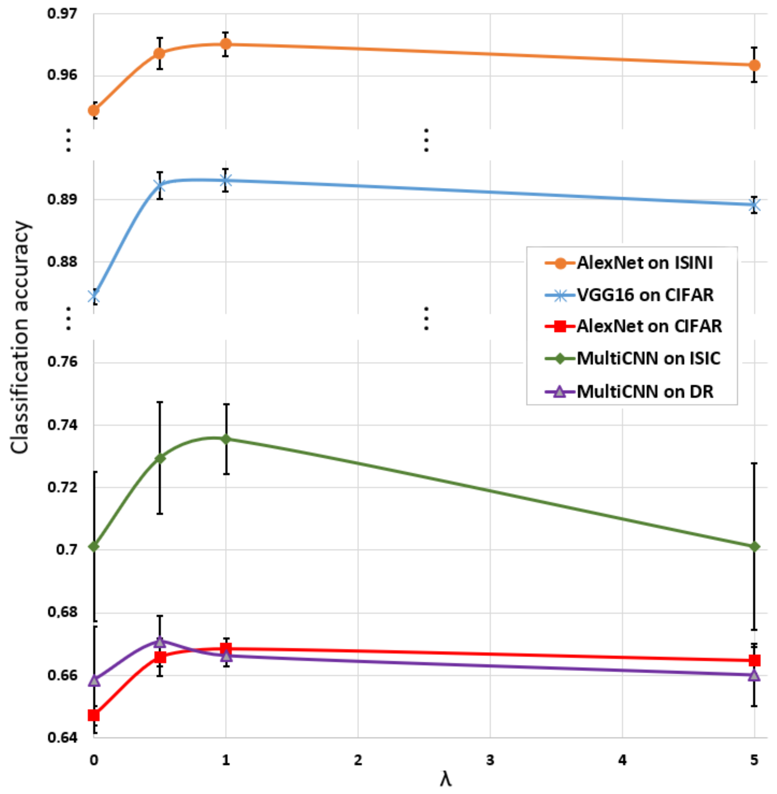
3.4. Discussion

As we saw in Section 3.3, the proposed penalization term makes the outputs of the members more diverse, which improves the final classification accuracy. Higher diversity is reflected in the number of jointly missed images. That is, double/triple misses reduce when the value of $\lambda$ increases. However, when the value of $\lambda$ goes over an optimal level, the overall accuracy of the ensemble starts to drop. The reason is that the approach focuses more on making the members more diverse than on the overall classification performance as we can see it, for example, in Figure 5. So we can consider $\lambda$ as a hyperparameter which should also be optimized similarly, for example, to the learning rate; thus, it should be carefully adjusted.

Regarding the details of implementation, several open-source libraries are available for machine learning and deep learning purposes, such as CNTK, Caffe2, PyTorch, TensorFlow, and Keras, which can be considered an API for the previously mentioned backend libraries. Our implementation was developed using TensorFlow (ver = 2.2.0) and TensorFlow-GPU (ver = 2.3.1) as backend for Keras. The CNNs VGG16, ResNet50, MobileNetV2 and GoogLeNet Inception-v3 were available as pre-trained models in Keras to build up our ensembles. The required AlexNet was not available in the core Keras library, so we composed this architecture from the necessary layers as published and trained it from scratch.

A general bottleneck of ensemble-based methods, especially in the case of CNN members, is that the number of model parameters increases to a large extent that requires the expansion of the training data set to avoid overfitting. Though we have not directly encountered this problem, a remedy can be to not fully pre-train the members, a solution which should leave some space for them to become diverse during their simultaneous training.Another common limitation of complex ensemble-based systems is that the training and optimization require high computational capacity. To mitigate this issue, we considered CUDA-based implementations running on GPU cards.

The fine-tuning and training steps were performed on a computer equipped with an NVIDIA TITAN RTX, and a GeFroce RTX 2080 Ti GPU card with 24 GB and 11 GB memories, respectively. The TITAN RTX (RTX 2080 Ti) has 16.31 (13.45) TFLOPs computational performance at single precision, 672.0 (616.0) GB/s of memory bandwidth, and 4608 (4352) CUDA cores. This 35 GB available memory was necessary when the ensemble networks were trained, and the total number of trainable and non-trainable parameters was 526,439,818. We used the mirrored strategies of TensorFlow for the complete ensemble network, which is typically used for training on one machine with multiple GPUs. The member CNNs were placed into the different GPU memories, so we shared the available memory among the network branches. The training time highly depends on the complexity of the model. For the individual networks, it is varied between 2 and 5 h, while the complex ensemble-based networks are trained for more than 16 h.

For a reliable evaluation, we fixed the same hyperparameter settings during the training stage of each setup. Namely, for optimizing the parameters of the individual CNNs and their ensembles, we trained the models over 100 epochs using the Adam optimizer with a learning rate of $1\times {10}^{-5}$. To avoid overfitting, we used $20\%$ of each training set as a cross-validation set. For each model, we preserved the parameters, reaching the highest accuracy on the validation set during the 100 epochs.

4. Conclusions

In this work, we introduced a new correlation penalty term to increase the diversity of individual CNN members to build up efficient ensembles from them. During training, the new term penalizes the cases when the members make wrong decisions simultaneously. In this way, our approach is technically similar to regularization, offering a trade-off between accuracy and diversity in the cost function. Accordingly, a parameter $\lambda$ is also introduced for weighing the correlation penalty consideration; the setting $\lambda =0$ completely switches it off. We gave a proper theoretical derivation of the new term and its derivative to support the efficient integration in the backpropagation process.

With this completion, we were able to remarkably improve the performance of previously proposed ensemble-based methods by generalizing them with the possible consideration of the new penalty term. Namely, our approach was evaluated on natural image classification problems with a specific interest on the clinical domain, including dermatology and retinal images as well. Accordingly, we fused popular CNN architectures by incorporating them into a super-network and adding the penalty term to the classification cost function. The ensembles trained using the new penalty term remarkably outperformed all the individual member CNNs and also the ensembles ignoring it. Moreover, a comparison with other state-of-the-art ensemble-based methods for the same classification task confirmed the efficiency of our approach.

Though our method was introduced for CNNs with corresponding image processing problems, the framework is sufficiently general for its possible applicability in other domains, too.