Article

Research on the Attack Strategy of Multifunctional Market Trading Oriented to Price

1
Department of Information Science and Engineering, Northeastern University, Shenyang 110819, China
2
Zhangjiakou Power Supply Company of Jibei Electric Power Company Limited, Zhangjiakou 075000, China
3
Navigation College, Dalian Maritime University, Dalian 116026, China
*
Author to whom correspondence should be addressed.
Mathematics 2023, 11(23), 4728; https://doi.org/10.3390/math11234728
Submission received: 12 October 2023 / Revised: 11 November 2023 / Accepted: 20 November 2023 / Published: 22 November 2023
(This article belongs to the Special Issue Mathematical Modeling for Parallel and Distributed Processing)

Abstract

:
In the context of energy transformation and power market system reform, it is crucial to address the network risks associated with enhancing the integration of the “Energy–Information–Market” paradigm. This necessitates research on multi-energy market trading modes and the corresponding offensive and defensive technologies. This paper proposes a novel approach centered around a node-local Energy Hub (EH) that represents large industrial users with diverse energy demands. To facilitate multi-energy two-way trading, a price-oriented Transactive Energy (TE) market clearing strategy is developed. Building upon this transaction network framework, a data-driven attack strategy targeting the state estimator of the Transmission System Operator (TSO) is introduced and implemented in two stages, encompassing real-time topology estimation and False Data Injection attacks. By leveraging Matrix Transfer Entropy (MTE), the optimal attack target is identified to disrupt the economic stability of the system and the profit of the attacker increases significantly. The proposed attack strategy is validated through simulations conducted on a 30-node system, yielding conclusive evidence of its effectiveness while offering vital insights for system defense.

1. Introduction

In various countries, the primary goal of power market development is to promote the transformation from a traditional power market to a multi-energy market. This shift is accompanied by the emergence of concepts such as the smart grid, distributed energy, and the Energy Hub [1,2]. The participation of user-side resources, particularly large industrial users represented by EHs, in the power market is of great significance. Through price signals, these resources can effectively utilize demand response capabilities, promote coordination and optimization among various energy sources, and contribute to the establishment of a secure multi-energy system. However, the close interactions among energy, information, and economy also introduces risks such as cyber attacks and information failure [3,4], which can disrupt the balance of market operations. It is therefore necessary to analyze and propose effective countermeasures to mitigate these risks. Doing so is fundamental to ensure the safe and stable economic operation of the multi-energy market.
Collaborative scheduling and energy trading among Energy Hubs (EHs) in the multi-energy market have gained increasing attention [5,6,7]. Three typical organization schemes for EH are analyzed, namely individual, shared, and aggregate schemes, in [8]. Furthermore, minimizing operating costs [9,10] and maximizing the energy efficiency [11] are common operational objectives for energy sharing among EHs. The interactions among different vendors in the operation process can be modeled as a precise potential game, bargaining cooperative game, or non-cooperative game [12,13]. Moreover, research related to energy sharing among productive consumers includes the P2P model and the leader–follower model. In the P2P structure, various approaches, such as auction models [14], pricing mechanisms [15], and multi-agent alliance frameworks [16], have been proposed to organize energy sharing among producers. On the other hand, the leader–follower structure often employs the Stackelberg game method to simulate the interaction between the leader and the follower. However, previous studies have not placed sufficient emphasis on the development of an effective autonomous pricing mechanism tailored to distributed multi-energy complementary systems. Such a mechanism is essential for accurately capturing the time-varying equilibrium conditions of Energy Hubs (EHs) and their individualized trading strategies.
The trading decision reference generated by the price signal plays a crucial role in commercial energy trading and requires special attention. As smart assets are typically located at the edge of the power network [17], it is necessary to optimize the market’s architecture to accommodate their specific characteristics and locations. In a study presented in [18], a two-level mathematical programming approach with equilibrium constraints is proposed to analyze the strategic behavior of profit-driven Energy Hubs (EHs) in the multi-energy market. At the lower level, the electricity and heating markets are cleared through location marginal prices, and contracts between energy centers and the two energy markets are determined. Another study suggests that the optimal scheduling of energy centers should consider electric, heat, and water requirements [19]. Simulation results demonstrate that EHs have a significant impact on the locational marginal prices (LMP) of electric nodes, indicating that the cost and benefits of EH devices are relatively similar.
From an economic perspective, the digitalization of the grid and the deregulation of the electricity market have created opportunities for profit-seeking cyber attacks. The accuracy of state estimation is crucial for real-time (RT) market auctions, but it is also vulnerable to network attacks. One typical network attack targeting state estimation is the False Data Injection (FDI) attack, which is characterized by its concealment, complexity, and destructive nature. The comprehensive impact of FDI attacks on energy markets is analyzed for the first time in [20]. An invisible FDI attack algorithm for state estimation is proposed, which enables attackers to gain monetary profits through maximum blocking transactions. Subsequently, a significant amount of research has been conducted on this topic [21,22,23]. The combination of false trading in the Day-Ahead (DA) markets with congestion model modifications is discussed as a means to generate profits in [24]. L. Xie te al. [25] analyzed the sensitivity of damaged sensors to Locational Marginal Prices (LMP) and identified the most sensitive bus and sensor. The mathematical relationship between the congestion cost and topology error is derived in [26], and the effect of topology error on LMP is expressed through a formula. Additionally, Q. Zhang et al. [27] discussed the opportunity for attackers to suppress the generation of distributed generators in order to obtain profits and analyzed the sensitivity of cuts and profits.
There has been research focused on launching profitable attacks, even without complete grid information [28,29]. To ensure profitability in the face of uncertain topological information, Rahman M A et al. [30] proposed a robust False Data Injection (FDI) attack that guarantees profits in the worst-case scenario. Additionally, R. Moslemi A M et al. [31] analyzed the impact of limited attacks on the power market operation. However, there are also studies that consider the completely unknown system structure. The attacker can infer the system topology through an independent component analysis and principal component analysis, as shown in [32]. The aforementioned research primarily analyzes the relationship between state estimation and the attack vector, using mathematical methods to infer system information or construct attack vectors. On a different note, Choi D-H et al. [33] introduced a novel approach by leveraging the transparency of the electricity market, which could be a promising choice.
The aforementioned attack research was conducted in the context of a single power market, which is inadequate for addressing the complexities of today’s multi-energy coupled energy market. Furthermore, there is a noticeable research gap regarding TE markets and their vulnerability to new attack strategies, particularly in the context of EH cluster-oriented network attack scenarios. Thus, it is of great significance to explore emerging attack strategies specifically tailored to the new TE market. The main contributions of this paper are summarized as follows:
  • The research focuses on developing a robust EH mathematical model to support energy management optimization and market transactions. Specifically, we propose a price-oriented TE market clearing strategy, tailored to the EH model, which enables multi-energy two-way trading between multiple EHs in a distributed, competitive manner. To solve the complex optimization problem associated with this strategy, a distributed algorithm based on the Nash equilibrium is employed.
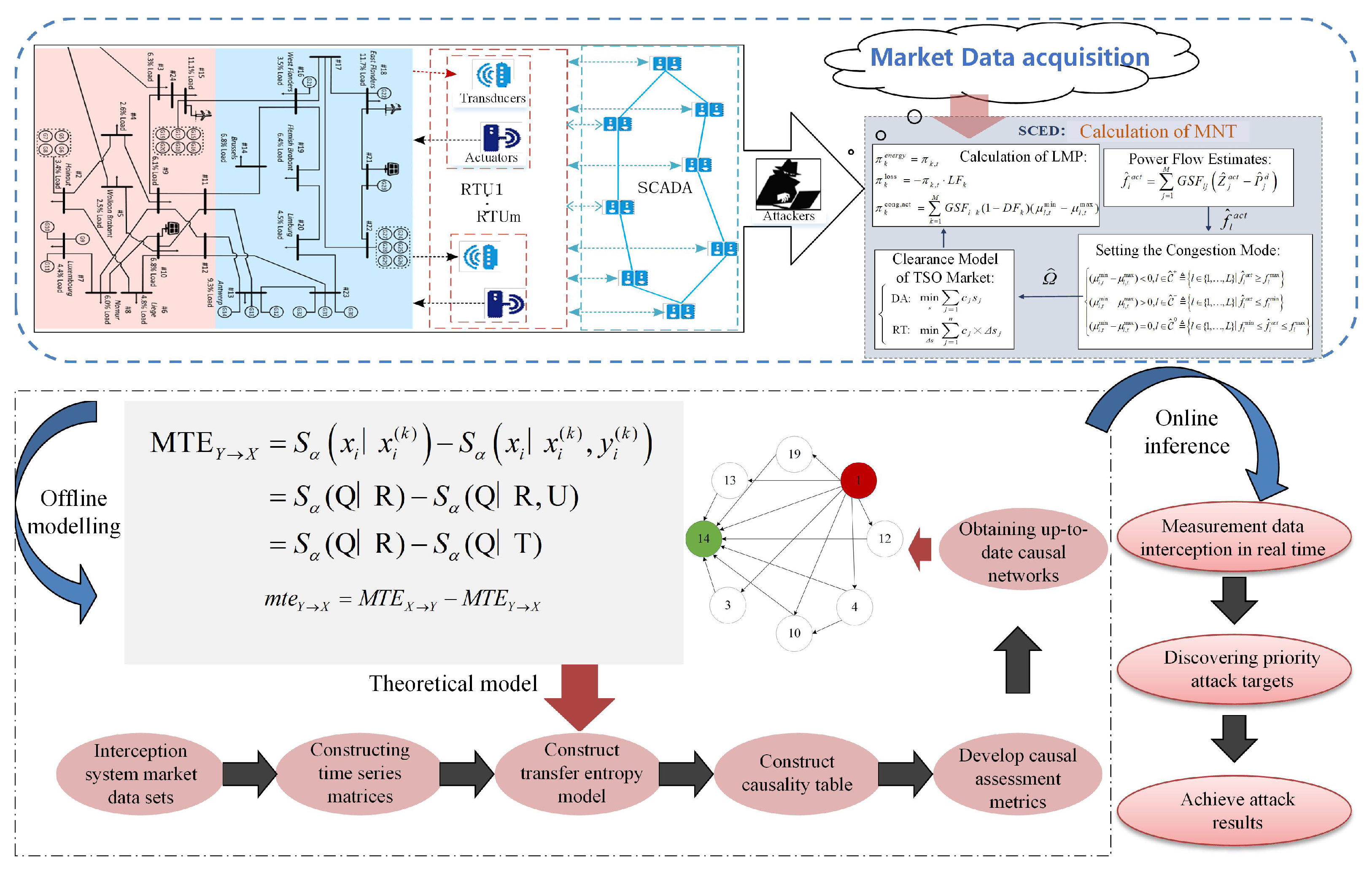
  • In order to target the state estimators of TSOs, we propose a two-stage attack strategy that is data-driven. In the first stage, a real-time topology estimation method is designed, making use of market data to provide the necessary conditions for subsequent successful False Data Injection (FDI) attacks. In the second stage, the attacker’s role is determined based on the attack mode that is feasible within the TE market environment. From the perspective of maximizing profit, we propose an objective function to guide the attacker’s actions.
  • In the attack strategy, we introduce an optimal method for identifying attack targets based on MTE. This method leverages market data for causal inference, enabling us to effectively identify potential targets for attack. By manipulating the TE market price information, our aim is to achieve attack targets that are both cost-effective and highly precise. This approach utilizes market data to its full potential and enhances the accuracy and efficiency of target identification in the attack strategy.

2. Price Oriented TE Market Model

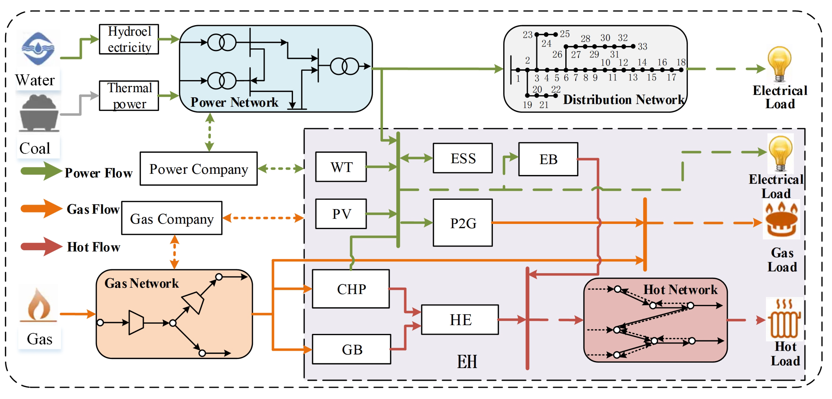
2.1. Structure of EH

The participation of user-side resources represented by Energy Hubs (EHs) in the power market is of significant importance in terms of providing flexibility and value and promoting the coordination and optimization of multi-energy sources. The node’s local energy community structure, illustrated in Figure 1, demonstrates how an EH can effectively coordinate and manage the generation, transmission, conversion, storage, and consumption of different types of energy within a given region. This allows the EH to offer users a range of energy products, such as electricity, gas, and heat. The EH can establish direct connections with power supply companies and gas companies, housing various types of renewable energy equipment, energy conversion devices, and energy storage systems [34,35,36].

2.2. TE Market Clearing Model Based on Price Guidance

2.2.1. TSO Market Trading Model

In this section, only the generation side quotations are considered. Therefore, a TSO clearing model is established based on the DCOPF (Direct Current Optimal Power Flow) model, which takes into account the losses. The goal of this model is to minimize the total generation cost, as shown in (1).
min o b j = t = 1 24 G Φ k M C G , k P G , k , t + G Φ k M C G , k , t u p Δ P G , k , t u p + C G , k , t d o w n Δ P G , k , t d o w n p Φ k N π p , k P p , k , t + p Φ k N π p , k u p Δ P p , k , t u p + π p , k d o w n Δ P p , k , t d o w n ,
s . t . G Φ k M Δ P G , k , t e l Φ k d Δ P e l , k , t + p Φ k N Δ P p , k , t = P l o s s : π k , t ,
Δ P G , k , t = Δ P G , k , t u p Δ P G , k , t d o w n ,
Δ P p , k , t = Δ P p , k , t u p Δ P p , k , t d o w n ,
P G , k , min P G , k , t + Δ P G , k , t P G , k , max ,
0 Δ P G , k , t d o w n r m p G , k d o w n ; 0 Δ P G , k , t u p r m p G , i u p ,
0 Δ P p , k , t u p ; 0 Δ P p , k , t d o w n ,
P p , k , max P p , k , t Δ P p , k , t P p , k , max ,
P l min G Φ k M G S F l k · P G , k , t + Δ P G , k , t p Φ k N G S F l k · P p , k , t + Δ P p , k , t e l Φ k d G S F l k · P e l , k , t + Δ P e l , k , t l Φ k N L G S F l k · D F k · P l o s s P l max : μ l , t min , μ l , t max .
where, in (1), the first two terms represent the operational and flexibility costs of the generator set. The third term represents the revenue earned by the Transmission Network (TN) through selling electricity to downstream Energy Hubs (EHs) in the energy market. The last term represents the cost incurred by the TN in procuring flexible resources from EHs in the market; (2) represents the flexible capacity balance equation. Constraints (3) and (4) describe the availability of flexible resources provided by the generator sets and EHs, respectively. Constraint (5) ensures that the sum of the energy and flexible resources provided by the generator does not exceed the maximum generation capacity. Constraint (6) states that the flexibility provided by the generator set should meet the ramp and ramp limit requirements. The flexibility limits provided by EHs to the TSO are described in constraints (7) and (8). Line power flow constraints are described in constraint (9).
In the above model, the LMP can be calculated using the Lagrangian function based on the dual variables of the equality constraints (2)–(4) and the inequality constraints (5)–(9), as shown in (10):
π L M P , k , t = π k , t π k , t L F k + k = 1 M G S F l k ( 1 D F k ) ( μ l , t min μ l , t max ) ,
where L F k is the network loss factor vector of the node, and L F k = 1 D F k . As can be seen from (10), the LMP can be divided into three parts: the marginal energy price, marginal network loss price, and marginal congestion price:
π k e n e r g y = π k , t π k loss = π k , t · L F k π k cong = k = 1 M G S F l k ( 1 D F k ) ( μ l , t min μ l , t max ) .

2.2.2. EH Transaction Model

In this section, it is assumed that there are N EH participants in the TE market for a potential game. Then, the set of participants is denoted as N = 1 , 2 , , N , the strategy of participants is denoted as τ i Γ i , and the benefit function is denoted as ψ i . The order represents a set of policy combinations for all participants. Then, a potential game can be defined as G = N , Γ i i N , ψ i i N , if and only if the game has a potential function that satisfies the following: for i N , τ i Γ i , x , z Γ i .
ψ i τ i , x ψ i τ i , z > 0 I f a n d o n l y i f P τ i , x P τ i , z > 0 ,
where τ i represents the policy combination set of other actors i except the actor i. Assuming that the vector ω = ω i i N is a positive real weighted vector, then for potential games, if there is a potential function that satisfies
ψ i τ i , x ψ i τ i , z = w i P τ i , x P τ i , z ,
the game is called the plus power game. If i N , ω i = 1 , then the game is a full potential game.
The energy transaction volume between the EH and the energy suppliers in the time period t is denoted as P i , γ , t r d = P i , e , t r d , P i , g , t r d γ e , g , a n d P i , γ , t r d 0 , indicating that the EH can only purchase energy in one direction from the energy suppliers. The transaction price is recorded as ρ i , γ , t r d = π L M P , i , e , t , ρ i , g , t r d γ e , g . Similarly, the energy transaction volume between EHs is denoted as P i , γ , t i k = P i , e , t i k , P i , g , t i k , P i , h , t i k γ e , g , h , and its transaction price is denoted as ρ i k , γ , t = π L M P , i , e , t , ρ i k , g , t , ρ i k , h , t γ e , g , h , i k . The benefit function of the EH in a period t consists of four parts: the energy use benefit, the income from supplying flexible resources to the TN, the equipment operation and maintenance costs, and the energy transaction cost. Then, the EH’s operation benefit function in a period is shown in (14):
ψ i N , t = γ = e , g , h t = 1 24 f i , γ , u + t = 1 24 π L M P , p , i u p Δ P p , i , t u p * + π L M P , p , i d o w n Δ P p , i , t d o w n * m W t = 1 24 f i , m , t t = 1 24 P i , e , t r d π L M P , i , e , t + P i , g , t r d ρ i , g , t r d γ = e , g , h t = 1 24 i = 1 N a i k , γ P i , γ , t i k ρ i k , γ , t P k , γ , t k i ρ k i , γ , t ρ i k , γ , t δ i k , γ P i , γ , t i k Δ t ,
where f s , γ , u is the energy efficiency; f i , m , t is the operating cost of type m equipment in the first EH at time t; π L M P , i , e , t is the electricity price of t period provided by the TSO for the ith EH; ρ i , g , t r d is the gas price for time t provided by the GMO for the ith EH; and A t = a i , k , t N × N is the adjacency matrix of the Transmission Network between EHs. a i , k , γ = 1 indicates that there is a transmission line of energy γ between the ith EH and the kth EH; if a i , k , γ = 0 , there is no transmission line. δ i , k , γ is the energy loss coefficient of the transmitted energy γ between the ith EH and the kth EH; P i , γ , t i k represents the power of the energy γ sent by the ith EH to the kth EH in time period t.
In addition, there is still a need to consider the constraints of the EHs and the energy supplier transactions, as well as the constraints of the transactions between the EHs.
0 P i , e , t r d P i , e , t r d , max , 0 P i , g , t r d P i , g , t r d , max ,
where (15) represents constraints on an EH’s purchase of electricity and natural gas from the energy suppliers. P i , e , t r d , max and P i , g , t r d , max represent the maximum amounts of electricity and natural gas purchased by the EH, respectively.
ζ s , γ , + P i , γ , t i k , min P i , γ , t i k ζ s , γ , + P i , γ , t i k , max ,
ζ s , γ , P i , γ , t k i , min P i , γ , t k i ζ s , γ , P i , γ , t k i , max ,
ζ s , γ , + ζ s , γ , + 1 ,
where P i , γ , t i k , max and P i , γ , t i k , min represent the upper and lower limits, respectively, of the energy l in the time period t between the ith EH and kth EH. And, they are both 0–1 binary variables. (16)–(18) ensure that at least one of the purchase and sale amounts of energy γ is zero, and they ensure that the purchase and sale of the same energy γ in a certain period of time between EHs will not occur at the same time.
In addition to meeting the physical and load constraints of the energy equipment model, an EH should also meet the energy supply and demand balance constraints:
P i , e , t r d + P i , e , t k i P i , e , t i k + P i , t w t + P i , t p v + P i , c h p , t out , e + P i , e s , t out P i , e b , t i n P i , p 2 g , t i n P i , e s , t i n Δ t = L i , e , t Δ t ,
P i , g , t r d + P i , g , t k i + P i , g , t k i P i , g , t i k + P i , p 2 g , t out P i , c h p , t i n P i , g b , t i n Δ t = L i , g , t Δ t ,
P i , h , t k i P i , h , t i k + ( P i , c h p , t out , h + P i , e b , t out + P i , g b , t out ) Δ t = L i , h , t Δ t ,
Equations (19)–(21) are respectively the power balance constraints of electricity/gas/heat in an EH. In order to facilitate the calculation, the unified gas power unit is kW, and the gas flow rate is converted into a power unit:
P i , g , t r d = Q g a s 3.6 × 10 6 g t ,
where Q g a s is the heat value per cubic meter of gas, and g t is the gas flow supplied by the gas supplier during the period t.
Combined with the above definition of the potential game, the potential function P ( τ ) of the potential game composed of multi-energy transactions among N EHs is established as
P ( τ ) = i = 1 N ψ i , t τ i ,
For the non-cooperative game between EHs, P i , γ , t i k = 0 is satisfied when the energy transaction between EHs is reached. If the strategies of other players are unchanged, the P i , γ , t i k in strategies x and z of participant i are unchanged, and for i N , τ i Γ i , x , z Γ i , there are
k i , k N u k τ i , x k i , k N u k τ i , z = 0 .
For the established potential function P ( τ ) , there is
P τ i , x P τ i , z = ψ i τ i , x + k i , k N ψ k τ i , x ψ i τ i , z + k i , k N ψ k τ i , z = ψ i τ i , x ψ i τ i , z + k i , k N ψ k τ i , x k i , k N ψ k τ i , z = ψ i τ i , x ψ i τ i , z .
Therefore, the multi-energy trading model between EHs conforms to the definition of the full potential game; that is, the game model is a full potential game.
The above models fully reflect the TSO–EH–GMO and EH–EH interactions. The TSO is considered to be responsible for centrally clearing the LMPs at each node of the power system, while the EHs trade electricity with the TSO at the price of the node where they are located and provide flexibility to the upstream grid by participating in the market.

2.3. Nash Equilibrium Distributed Solution

In order to solve the Nash equilibrium, the ADMM is used in this section to convert the benefit maximization problem into a cost minimization problem; that is, the cost function is the opposite of the benefit function ψ i , as shown in (26):
C i , t = ψ i , t ,
When the potential function P reaches its maximum value, the game can achieve the Nash equilibrium. That is, to obtain the minimum value of the inverse C p of the potential function, the optimization problem required to solve the function can be converted to Equation (27):
M i n C p = P ( τ ) = i = 1 N C i , t ψ i S t . τ i Γ i P i , γ , t i k τ i , i = 1 N P i , γ , t i k = 0 , γ { e , g , h } ,
where, the EH’s strategy τ i can be divided into three parts: the first part is the transaction variable x i = P i , e , t i k , P i , g , t i k , P i , h , t i k among EHs, the second part is the transaction volume y i = P i , e , t r d , P i , g , t r d , Δ P p , k , t u p , Δ P p , k , t d o w n with energy suppliers, and the third part is the internal equipment output z i = P i , t wt , P i , t p v , P i , c h p , t out , e , P i , c h p , t out , h , P i , e b , t out , P i , g b , t out , P i , p 2 g , t out , P i , e s , t of the EH.
Based on the potential game model established in this paper, the sub-objective function is the comprehensive cost function of each EH participant, and the overall objective function C p is the inverse of the potential function P, so there is no need for further splitting. The ADMM algorithm is rewritten into a form that is suitable for solving the Nash equilibrium in potential games, as shown in (28):
x i ν + 1 , y i v + 1 , z i v + 1 = arg min x i , y i , z i C i , t x i , y i , z i + ( ρ / 2 ) x i x i v + x ¯ v + ξ v 2 2 x ¯ v + 1 = 1 N i = 1 N x i v + 1 ξ v + 1 = ξ v + x ¯ v + 1
where x i ν + 1 represents the ( v + 1 )th decision variables of the ith EH, and ξ v + 1 is the dual variable. Each time the TSO clears π L M P , i , e , t and the EH, there is a unique Nash equilibrium after the potential game. The proposed Nash equilibrium solution process based on the ADMM algorithm is shown as follows (Algorithm  1).
Algorithm 1 Solving the potential game based on the ADMM.
Input: 
N, M, k, v = 0 , equipment parameter, load information, external conditions, x i v , y i v , z i v , π L M P , i , e v , ρ ,
Output: 
x i * , y i * , z i * , C p *
1:
Repeat
2:
   TSO and GMO;
3:
   Receive transactions from EHs: y i v = P i , e , t r d , v , P i , g , t r d , v , Δ P p , k , t u p , v , Δ P p , k , t d o w n , v ;
4:
   Update the power output P G , k , t v + 1 of the generator set on the TN and the power consumption y i v + 1 of the EH connected to the TN and natural gas network;
5:
   The node electricity price for the LMPs is calculated by (10): π L M P , i , e v ;
6:
   Send y i v + 1 , π L M P , i , e v + 1 and ρ i , g , t r d to EHs through the energy trading platform;
7:
   EHs i N ;
8:
   Receive y i v + 1 , π L M P , i , e v + 1 , ρ i , g , t r d from TSO and GMO;
9:
   Update the EHs’ loading information and external conditions;
10:
   The comprehensive cost C p v of the EHs is calculated by (27);
11:
   The policy sets x i v + 1 , y i v + 1 , z i v + 1 , and x ¯ v + 1 , ξ v + 1 are updated by (28);
12:
   When we reach the Nash equilibrium, v = v + 1 ;
13:
End
Multi-energy bidirectional transactions are carried out among multiple EHs in a distributed and competitive way, and the distributed algorithm is used to solve the Nash equilibrium. The following example analysis verifies the superiority of the above model in dealing with multi-energy two-way transactions.

3. A Data-Driven Attack Strategy against TSO State Estimators

3.1. A Data-Driven Topology Estimation Method

Transparency in market data plays a crucial role in fostering a competitive and efficient energy environment. However, it is important to balance transparency with the need to protect critical physical system information. In many markets, the publicly available information is primarily focused on Locational Marginal Prices (LMP), while information about the physical infrastructure is often delayed or incomplete. In this context, estimating the network topology from published LMP data becomes a suitable option.
In order to facilitate subsequent calculations, π c o n g in (11) is expressed as a vector, as follows:
π c o n g = G S F G S F · D F · e T T u ,
The relationship between π c o n g and G S F is clearly shown in (29), and the more explicit relationship between the price information and topology is as follows:
π c o n g = G S F G S F · D F · e T T · u = ( G S F T e · D F T · G S F T ) · u = ( D A L 1 ) T · u e · D F T · ( D A L 1 ) T · u = L 1 A T D · u e · D F T · L 1 A T D · u ,
From (30), we know that π c o n g is related to the topologically dependent matrix ( L , D , A ) , while the Jacobian matrix H consists of L and ( D , A ) . Therefore, in this section, π c o n g is divided into two parts according to L and ( D , A ) . Then, an intermediate variable κ = A T D · u = H 2 T · u is introduced, and the historical data π c o n g and κ are expressed as Π = π 1 , , π t and K = κ 1 , , κ t , respectively, according to the time series. In addition, in order to meet the recovery conditions, they are converted to solve the SDP problem, and the updated (30) is as follows:
H 1 · Π = K H 1 · e · D F T · H 1 1 · K ,
In addition, under reasonable market conditions, the line is not congested at all times, that is, u is sparse, and ( D , A ) is a sparse matrix, so K = κ 1 , , κ t is sparse, and H 1 · Π is also sparse.
Based on the sparsity of H 1 , H 1 · Π and H 1 · e , we use compressed sensing to express the recovery model as an optimization problem. Mathematically, the goal of compressed sensing is sparse reconstruction, i.e., solving the following sparse minimization problem:
min s s 0 s . t . y = Φ Ψ s .
Equation (32) is an NP-hard underdetermined problem. We apply the l 1 -norm to the sparse vector H 1 · e and the l 2 , 1 -mixed norm to the sparse matrices K and H 1 . The objective function is as follows:
min H 1 K 2 , 1 + κ 1 H 1 2 , 1 + κ 2 H 1 e 1 κ 3 log H 1 ,
Equation (33) is composed of H 1 , K and H 1 · e , where K and H 1 · e are always sparse, regardless of the size of the system. The topological estimate H is updated each time the price vector is published. For big data processing, the ADMM solution is given as follows:
min x X , z Z t = 1 T f t ( x ) + g ( z ) s . t . A x + B z = c ,
The original iteration process of ADMM is as follows:
x t + 1 = arg min x X f t ( x ) + y t A x + B z t c + ρ 2 A x + B z t c 2 + η 2 x x t 2 z t + 1 = arg min z Z g ( z ) + y t A x t + 1 + B z c + ρ 2 A x t + 1 + B z c 2 y t + 1 = y t + ρ A x t + 1 + B z t + 1 c ,
By substituting the inner product of y and A x + B z = c into the quadratic term, we obtain
x t + 1 = arg min x X f t ( x ) + ρ 2 A x + B z t c + y t T / ρ 2 + η 2 x x t 2 z t + 1 = arg min z Z g ( z ) + ρ 2 A x t + 1 + B z c + y t T / ρ 2 y t + 1 = y t + ρ ( A x t + 1 + B z t + 1 c ) ,
By replacing y t / ρ with y ^ t , we obtain
x t + 1 = arg min x X f t ( x ) + ρ 2 A x + B z t c + y ^ t 2 + η 2 x x t 2 z t + 1 = arg min z Z g ( z ) + ρ 2 A x t + 1 + B z c + y ^ t 2 y ^ t = y ^ t + A x t + 1 + B z t + 1 c ,
To apply the ADMM, for each term and each constraint in the objective function, we introduce H 1 , 1 = H 1 , 2 = H 1 , 3 = H 1 , 4 = H 1 , 5 and H 1 , 1 e = b as new optimization variables and write the problem as
min H 1 , 3 B 3 , H 1 , 4 B 4 , H 1 , 5 B 5 , b S t = 1 T f t H 1 , 1 + g 1 H 1 , 2 + g 2 H 1 , 3 + g 3 H 1 , 4 + g 4 H 1 , 5 + g 5 ( b ) s t . H 1 , 1 H 1 , 2 = 0 ; H 1 , 1 H 1 , 3 = 0 ; H 1 , 1 H 1 , 4 = 0 ; H 1 , 5 H 1 , 1 = 0 ; H 1 , 1 e b = 0 ; H 1 , 1 Π = K ,
where, f t H 1 , 1 = K l 2 , 1 , g 1 H 1 , 2 = κ 1 T H 1 , 2 l 2 , 1 , g 2 H 1 , 3 = κ 3 T log H 1 , 3 , g 3 H 1 , 4 = 0 , g 4 H 1 , 5 = 0 , g 5 ( b ) = κ 2 T b l 1 , B 3 = { H 1 0 } , B 4 = { H 1 I } , B 5 = H 1 ( i , j ) = v , { i , j , v } D t , S = { b 0 } .
Let the Lagrange multiplier of (38) be represented by λ 12 λ 13 λ 14 λ 15 λ 16 and λ 10 . Then, the recursive iteration process is described as follows:
H 1 , 1 t + 1 = arg min H 1 , 1 K 1 + ρ 2 H 1 , 1 H 1 , 2 t + λ 12 t F 2 + ρ 2 H 1 , 1 H 1 , 3 t + λ 13 t F 2 + ρ 2 H 1 , 1 H 1 , 4 t + λ 14 t F 2 + ρ 2 H 1 , 1 H 1 , 5 t + λ 15 t F 2 + ρ 2 H 1 , 1 e b t + λ 10 t 2 2 + η 2 H 1 , 1 H 1 , 1 t F 2 ,
H 1 , 2 t + 1 = arg min H 1 , 2 κ 1 T H 1 , 2 l 2 , 1 + ρ 2 H 1 , 1 t + 1 H 1 , 2 + λ 12 t F 2 ,
H 1 , 3 t + 1 = arg min H 1 , 3 B 3 κ 3 T log H 1 , 3 + ρ 2 H 1 , 1 t + 1 H 1 , 3 + λ 13 t F 2 ,
H 1 , 4 t + 1 = arg min H 1 , 4 B 4 ρ 2 H 1 , 1 t + 1 H 1 , 4 + λ 14 t F 2 ,
H 1 , 5 t + 1 = arg min H 1 , 5 B 5 ρ 2 H 1 , 1 t + 1 H 1 , 5 + λ 15 t F 2 ,
b t + 1 = arg min b S κ 2 T b l 1 + ρ 2 H 1 , 1 t + 1 e b + λ 10 t 2 2 ,
K t + 1 = S ρ 1 H 1 , 1 T + 1 Π + λ 16 t , S β ( x ) : = x β sign ( x ) , | x | > β 0 , | x | β ,
λ 12 t + 1 = λ 12 t + H 1 , 1 t + 1 H 1 , 2 t + 1 ; λ 13 t + 1 = λ 13 t + H 1 , 1 t + 1 H 1 , 3 t + 1 λ 14 t + 1 = λ 14 t + H 1 , 1 t + 1 H 1 , 4 t + 1 ; λ 15 t + 1 = λ 15 t + H 1 , 1 t + 1 H 1 , 5 t + 1 λ 16 t + 1 = λ 16 t + H 1 , 1 t + 1 Π K t + 1 ; λ 10 t + 1 = λ 10 t + H 1 , 1 t + 1 e b t + 1 ,
In short, the attacker can implement the iterative process of (39)–(46) through the ADMM algorithm to realize the grid topology restoration of the node admittance matrix. Then, the approximate real grid admittance matrix model L ˜ a c t is shown in (47).
H ˜ 1 a c t = L ˜ a c t = L 11 L 1 n L n 1 L n n + Δ L 11 Δ L 1 n Δ L n 1 Δ L n n ,
The first term is the real admittance matrix. The second term Δ y is the error between the actual model and the model estimated by the attacker. The elements corresponding to the real power injection are shown in (48).
P i n j θ i = j = 1 , j i M V i V j G i j a c t cos θ i j B i j a c t sin θ i j P i n j θ j = V i V j G i j a c t sin θ i j B i j a c t cos θ i j P i n j V i = j = 1 , j i M V j G i j a c t sin θ i j + B i j n a c t cos θ i j P i n j V j = V i G i j a c t sin θ i j + B i j a c t cos θ i j ,
These elements form the attacker’s Jacobian matrix H ˜ a c t , as shown in (49).
H ˜ a c t = P i n j θ P i n j V P l l θ P l l V .
where the estimated matrix H ˜ a c t exhibits a sparse structure that closely resembles the real matrix H. The locations of non-zero elements in the matrix correspond to the existence of transmission lines. Consequently, the evaluation process can be divided into two steps. Firstly, the elements of the estimated matrix H ˜ a c t are categorized into zero and non-zero classes. Secondly, the positions of non-zero elements in the real matrix H are compared with those in the estimated matrix H ˜ a c t to assess the difference.

3.2. The Attacker Model in the TE Market Environment

In this section, the primary focus lies in identifying the attacker and the target of the attack in the context of energy trading within the TE market. Given the extensive information exchange among numerous market participants, including IoT-integrated EHs, diverse forecasters, market operators, producers, and consumers, it becomes crucial to consider the potential presence of adversaries and malicious users who may assume the role of attackers during the energy trading process and the provision of flexibility.

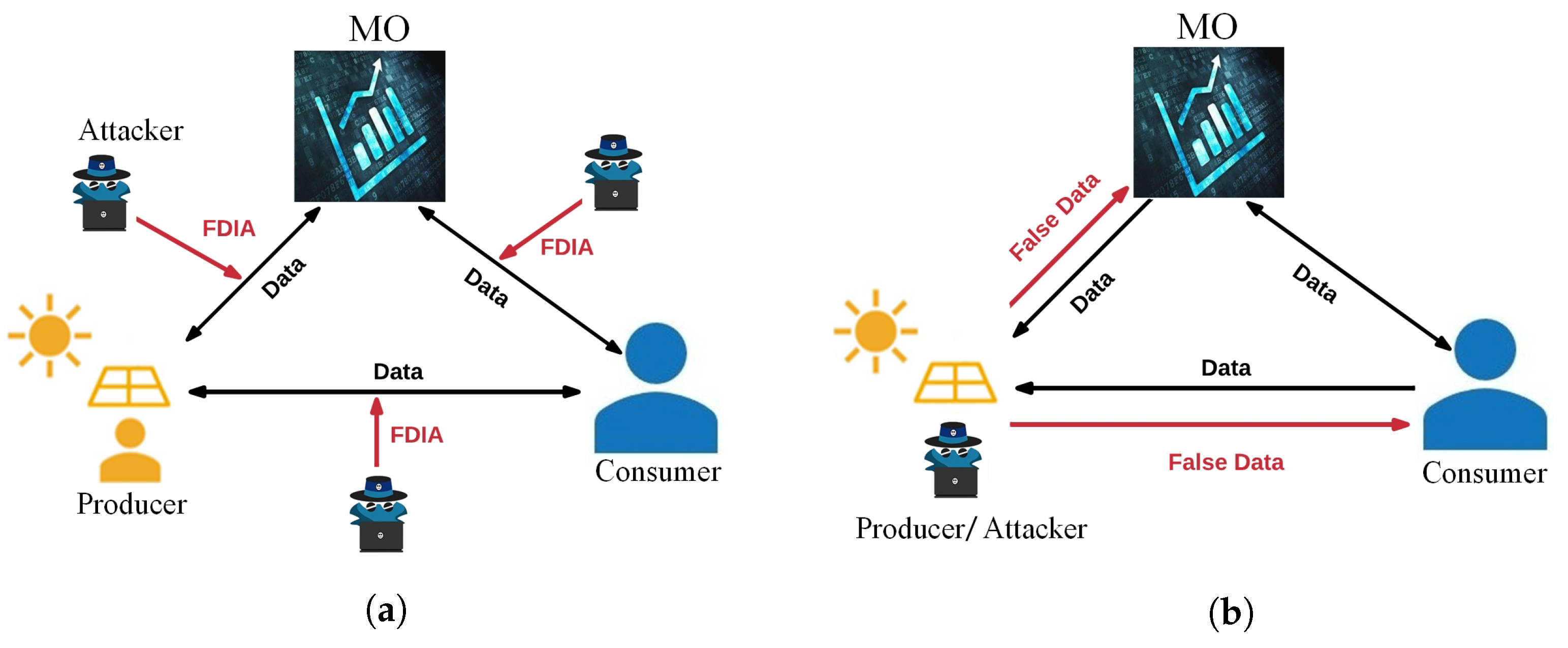
3.2.1. Role Analysis of the Market Attacker

Figure 2 depicts the role that an attacker can play in the TE market, and Figure 2a depicts the communication channels of an FDI attack by manipulating the price signals exchanged between producers, consumers, and market operators in order to cause economic damage to all market participants or disrupt normal market operations. Figure 2b depicts the malicious user role, where malicious consumers act as attackers and provide false data to TE market operators or peers in order to increase their own financial gain.
As mentioned above, in all market components, communication channels, smart devices, and bad users can act as the main vectors for executing different cyber attacks due to weak security mechanisms and direct access to the system. Therefore, in this section, we divide attacks into three categories based on the vulnerable market components of the TE market: (1) attacks through communication channels; (2) attacks through equipment; and (3) attacks by malicious users.

3.2.2. Attack Model of the Virtual Bidder

In the RT market, based on state estimates at the end of each interval, the TSO estimates the power generation of bus j and the P j g and P j d of the load. The power flow estimated by the TSO through each transmission line l is shown in (50):
P ^ l = j = 1 M G S F l j P ^ j g P ^ j d ,
When the estimated flow exceeds the limit, we consider the branch to be congested. When the line currents belong to different congestion sets, the congestion price part is expressed as shown in (51).
( μ l , t min μ l , t max ) < 0 , l C ^ + = Δ l { 1 , , L } P ^ l P l max ( μ l , t min μ l , t max ) > 0 , l C ^ = Δ l { 1 , , L } P ^ l P l min ( μ l , t min μ l , t max ) = 0 , l C ^ 0 = Δ l { 1 , , L } P l min P ^ l P l max ,
In the RT market, FDI attacks can inject false data in bidding, line rating, the demand response, and other aspects, which affects the congestion price π c o n g of the RT market operation. Virtual bid transactions are summarized in Table 1.
The VB revenue objective function can be constructed as a function of π L M P D A and π L M P R T , as (52):
U π L M P D A , π L M P R T , a = π i , L M P R T π j , L M P R T + π j , L M P D A i , L M P D A · P d = l L + G S F l , i ( 1 D F i ) G S F l , j ( 1 D F j ) · ( μ l , t min μ l , t max ) + l L G S F l , j ( 1 D F j ) G S F l , i ( 1 D F i ) · ( μ l , t min μ l , t max ) + π j , L M P D A π i , L M P D A · P d ,
If the three conditions of (53) are met, the payoff is always positive.
( 1 ) π j , L M P DA π i , L M P DA 0 ( 2 ) l L + = Δ l { 1 , , L } : G S F l , i ( 1 D F i ) > G S F l , j ( 1 D F j ) , P ^ l a c t P l min ( 3 ) l L = Δ l { 1 , , L } : G S F l , i ( 1 D F i ) < G S F l , j ( 1 D F j ) , P ^ l a c t P l max ,
Since P ^ l a c t follows a Gaussian random distribution, full satisfaction of the second and third conditions of (53) cannot be guaranteed. However, the attack vector a can be designed to maximize the probability of satisfying both conditions. This paper introduces δ as the profit confidence, and in order to create (or eliminate) congestion on line l, the attackers design their attacks such that P ^ l a c t P l max + δ ( P ^ l a c t P l max δ ) . In addition, the chance constraint η ( 0 , 1 ) with an allowable confidence interval is added to provide the optimal injection vector under uncertain conditions, as shown in (54).
P ^ l a c t P l min + δ η , l L + P ^ l a c t P l max δ η , l L ,
At the same time, δ needs to be maximized to increase its chances of achieving the congestion it seeks. Market attacks can therefore be seen as solving the following opportunity constraint problem:
max δ P ^ l a c t P l min + δ η , l L + P ^ l a c t P l max δ η , l L δ > 0 , 0 < η < 1 .
The performance of FDI attacks requires the attacker to modify the sensor measurements and write access, thus providing the instructions shown in Figure 3. A resource-constrained VBS may want to minimize the number of sensors it has to compromise to perform an FDI attack, or equivalently, maximize the sparsity of the attack.
Although the above method can find the attack vector a, the sparsity and effectiveness of the attack vector cannot be satisfied at the same time. This paper not only considers the energy limit of the enemy but also considers the optimal selection of the attack target. The importance of the attack target is higher than the attack type, and an important trade-off between the sparsity and effectiveness of the attack vector a has been achieved.

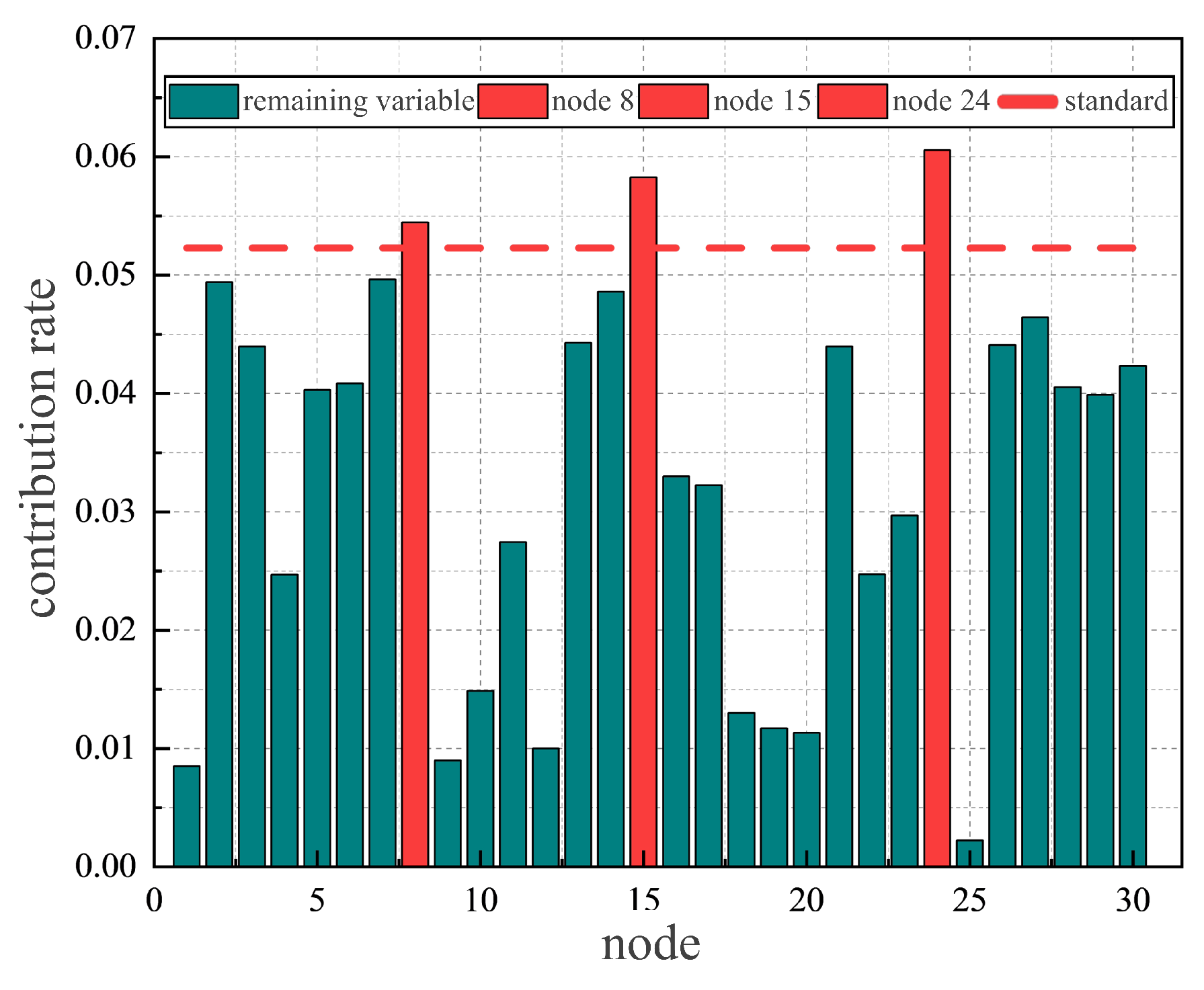
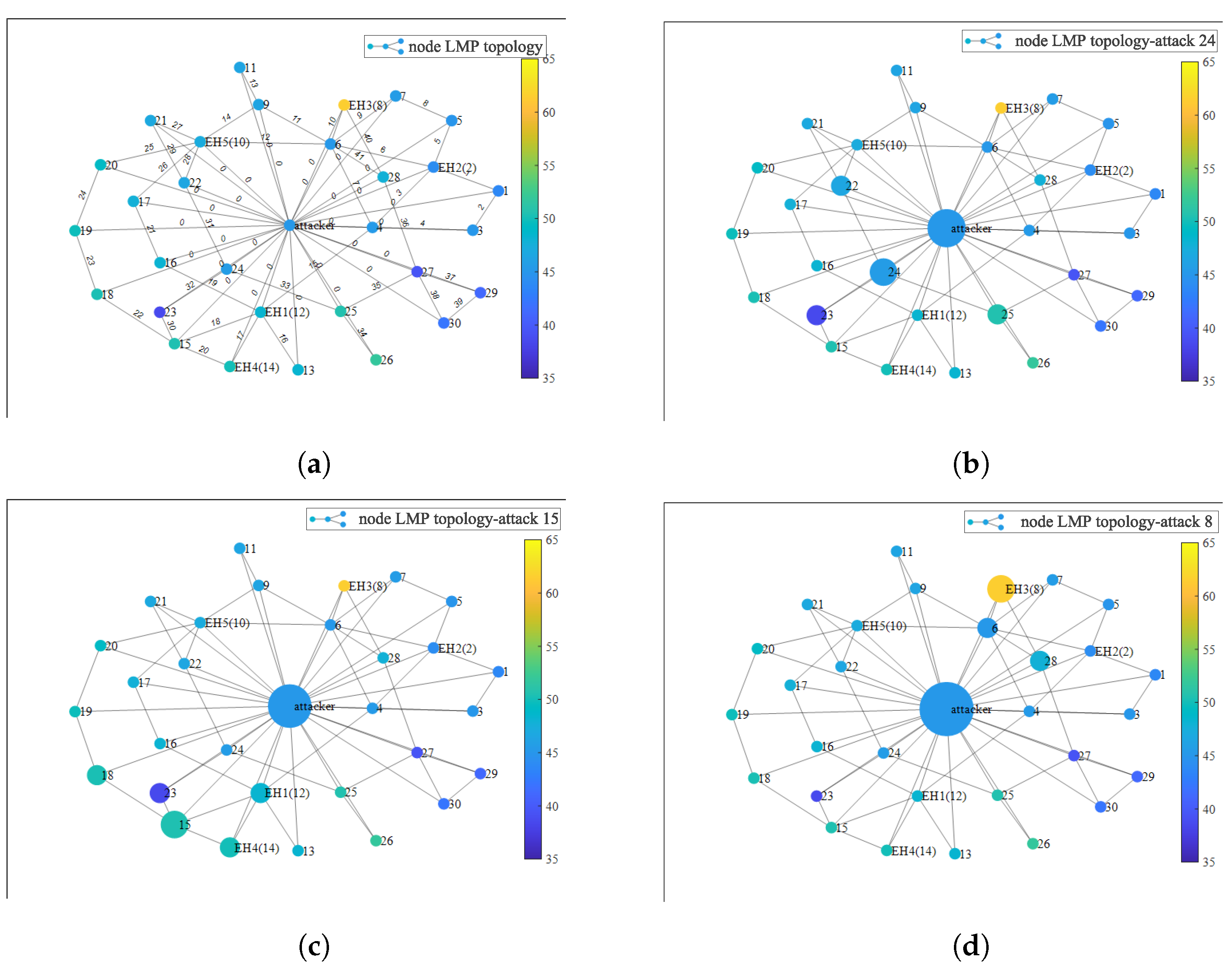
3.3. Optimal Attack Target Identification Method Based on MTE

Due to the high computational complexity of transfer entropy (TE), the calculation of a large amount of historical measurement data will increase the storage and computation burden [37]. To solve the above problems, we employ causal inference based on the Matrix Transfer Entropy (MTE) method, which can be used for two variables with linear or non-linear causal relationships. Compared with the traditional TE method, this method is more robust. The computational complexity of the MTE method is not high because it ignores the estimation of the probability density function of the variable. The calculation of the MTE primarily relies on the matrix entropy, edge entropy, and conditional entropy. The matrix entropy is obtained by taking the logarithm of the trace of the Gram matrix. Likewise, the edge entropy is obtained by taking the logarithm of the trace of the Hadamard product of two Gram matrices. Conditional entropy, on the other hand, is determined as the difference between the first two measures mentioned above. Similarly, we can define the MTE from X to Y:
M T E X Y = S 2 y i | y i ( k ) S 2 y i | y i ( k ) , x i ( k ) ,
where S 2 y i | y i ( k ) represents the second-order matrix entropy of the variable y; S 2 y i | y i ( k ) , x i ( k ) represents the edge ME between variable y and variable x; k is the implant dimension.
In the same way as determining the direction of the transfer entropy causality, the direction of causality between X and Y can also be well judged by the difference between the two TEs:
m t e Y X = M T E X Y M T E Y X ,
In order to better infer the relationship between the injection of the attack vector a and the revenue U of the VB, according to (50)–(52), for all buses π L M P and measurement data z, the revenue U can be expressed in the compound function form of (58):
U = h ( π L M P ( z m ( a ) ) ) ,
π L M P , N = f N z 1 , z 2 , , z m ,
z M ˜ = g M ˜ a 1 , a 2 , , a m ,
where U represents th eVB revenue; π L M P = [ π L M P , 1 , π L M P , 2 , , π L M P , Y ] T indicates the LMP on the bus. z M ˜ and a M ˜ are the measurements of the sensor and their corresponding attack vectors respectively. h · , U. f N · and g M ˜ · are vector functions.
The main objective of this paper is to reflect the degree of change in the attacker’s benefit when any sensor measurement value in the entire Transmission Network is changed by the injected attack vector:
Λ l i , j = U a ,
where Λ l i , j represents the degree of profitability to quantify the amount of increase/decrease in the profit and by manipulating the appropriate virtual bid nodes or lines in the TE market. According to the chain rule, (61) can be written as
Λ l i , j = U a = U π · π z · z a ,
In the RT power market, the DC state estimator is used. Then the measurement data z only include the active power P i injected by the node and the active power P i j of the line, that is, z = P i , P i j T . While P i and P i j can be expressed by the power transfer factor matrix G S F , in this case, it can be expressed by using the power of m group nodes and the branch power flow in the time period t m :
P 12 t 1 P 12 t 2 P 12 t 3 P 13 t 1 P 13 t 2 P 13 t m P i j t 1 P i j t 2 P i j t i j L × t m = G S F L × Y · P 1 t 1 P 1 t 2 P 1 t 3 P 2 t 1 P 2 t 2 P 2 t m P Y t 1 P Y t 2 P Y t i j Y × t m ,
According to the relationship analysis among the variables of the measurement data in (63), if the causal relationship between the injected power of nodes is inferred through the TME, the information entropy between nodes can be obtained, and then the causal relationship with the line power can be obtained.
Suppose that the attacker injects the attack vector a into the injected power P i ( P j ) of node i ( j ) , then the change in P i ( P j ) of node i ( j ) before and after the attack is Δ P i a c t ( Δ P j a c t ) , the change in P i j before and after the attack is Δ P i j a c t , the change in π i ( π j ) before and after the attack is Δ π i a c t ( Δ π j a c t ) , and the change in the corresponding revenue function U is Δ U . At this time, the expression relationships among the four are as follows:
Δ P i a c t = P i + a i P i Δ P j a c t = P j + a j P j Δ P i j a c t = G S F i j i Δ P i a c t + G S F i j j Δ P j a c t Δ π L M P , i a c t = G S F i j i · Δ μ i Δ U = Δ ξ · P d
It can be seen that the change in data corresponding to nodes can better reflect the causal relationships among nodes. The specific flow of the optimal attack target identification method based on the MTE is shown in Figure 4. First of all, a time series matrix is constructed for the obtained market data, and then the causal relationships among variables are inferred based on the MTE model, and the causal relationship table is constructed as a reference premise. Then, the causal evaluation index is constructed to select the optimal attack target.

4. Simulation Results

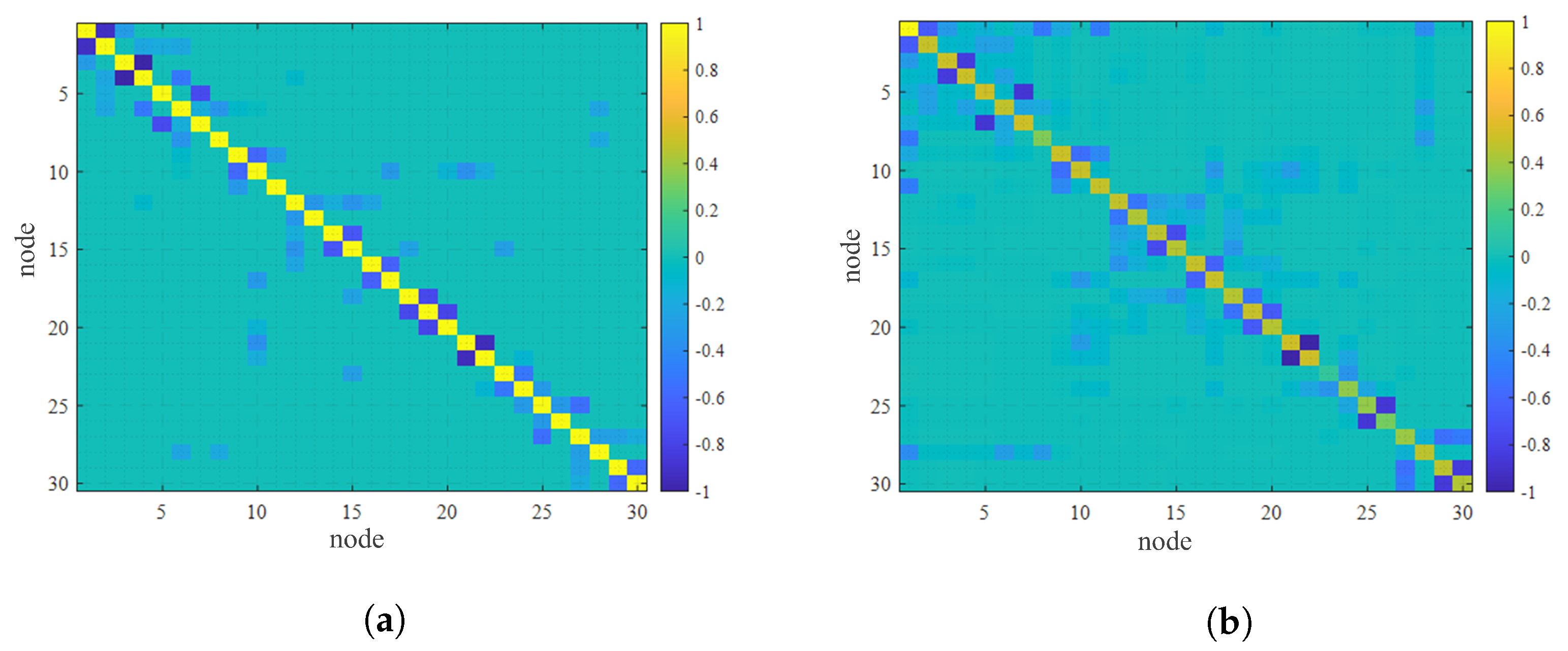
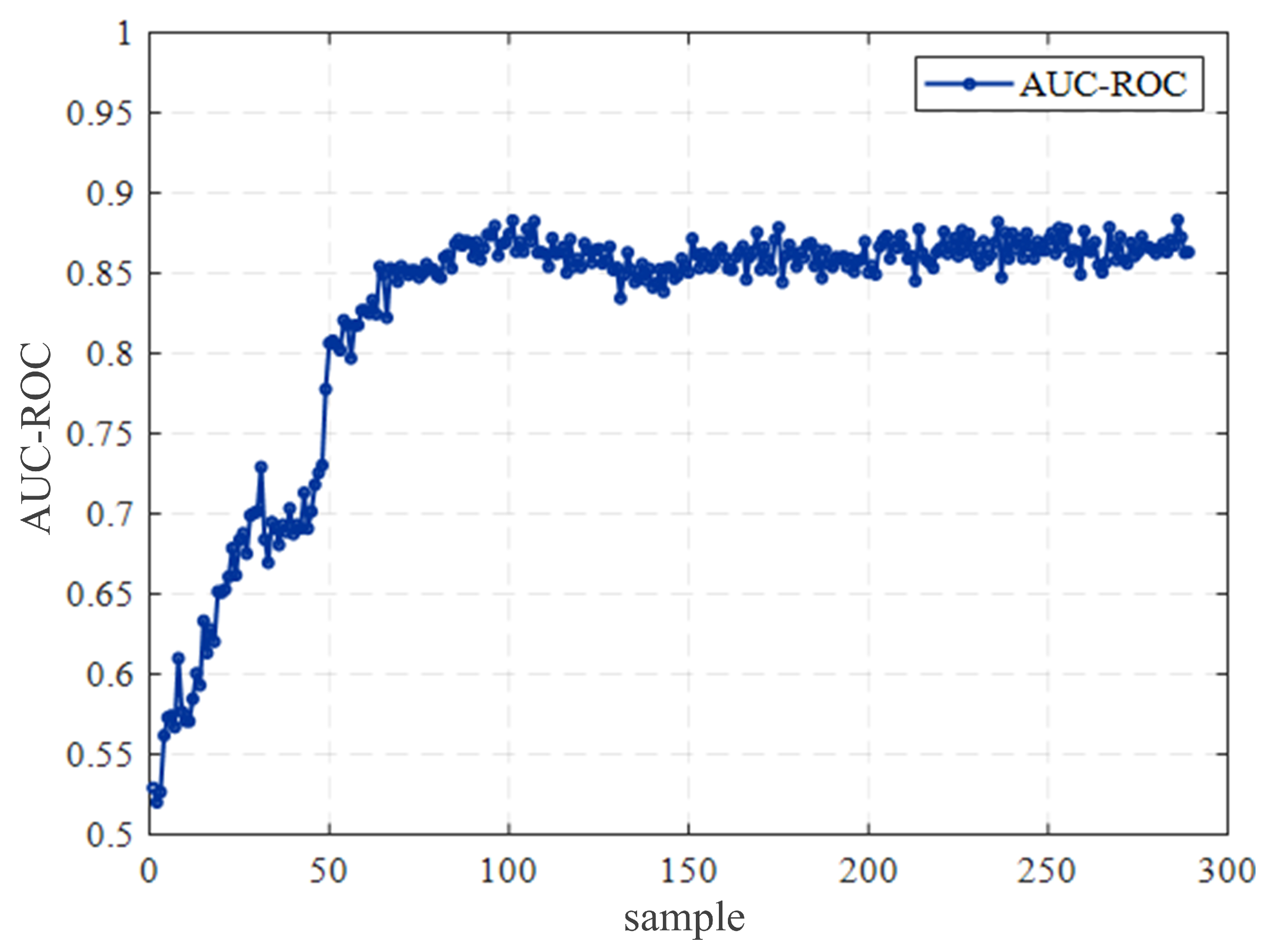
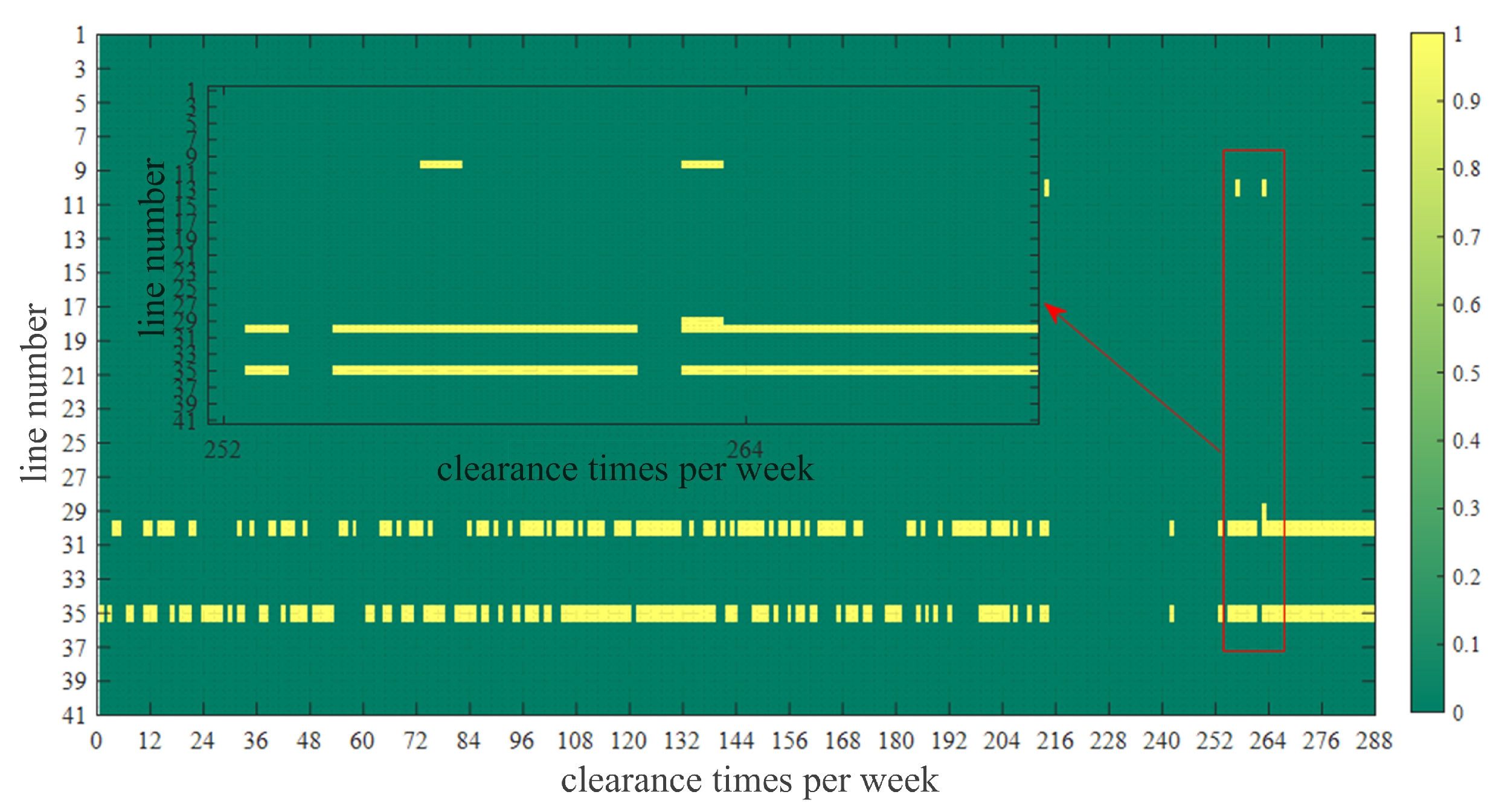
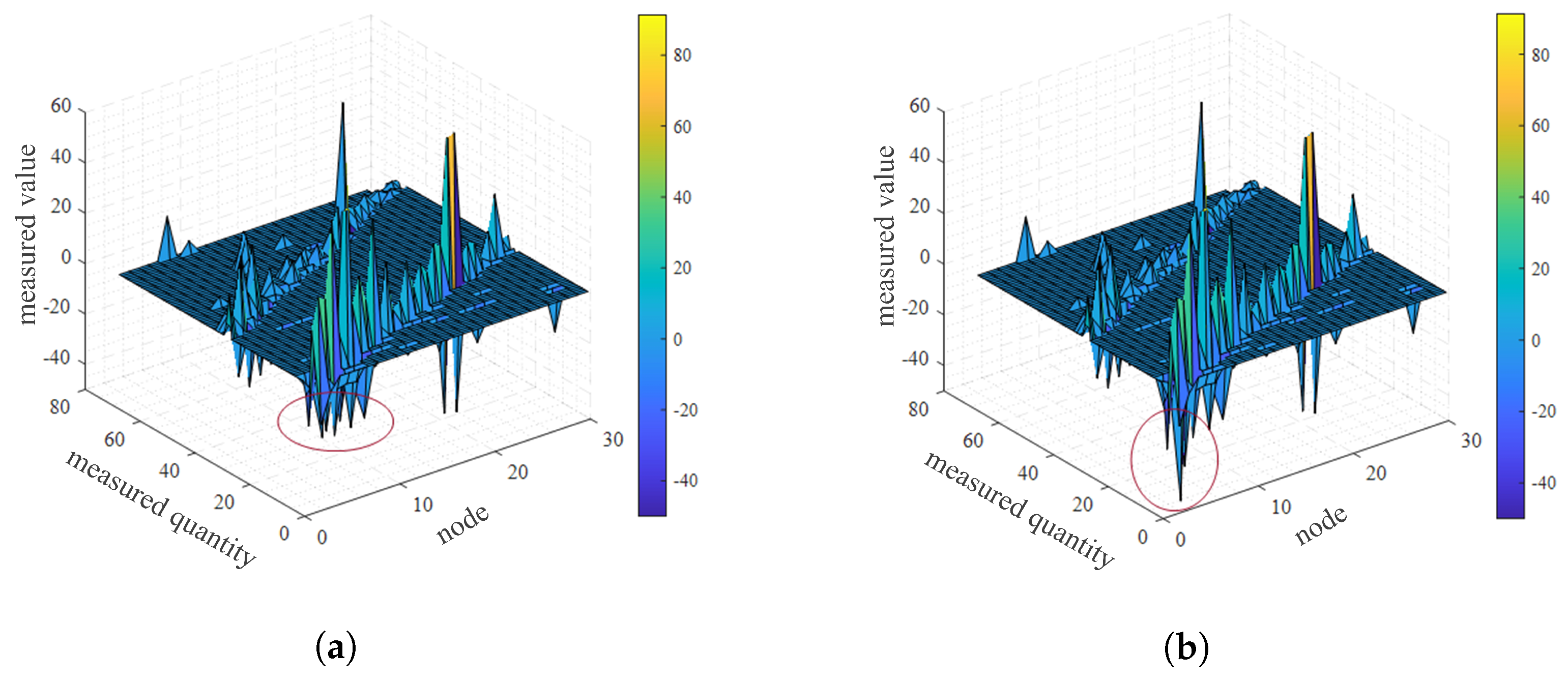
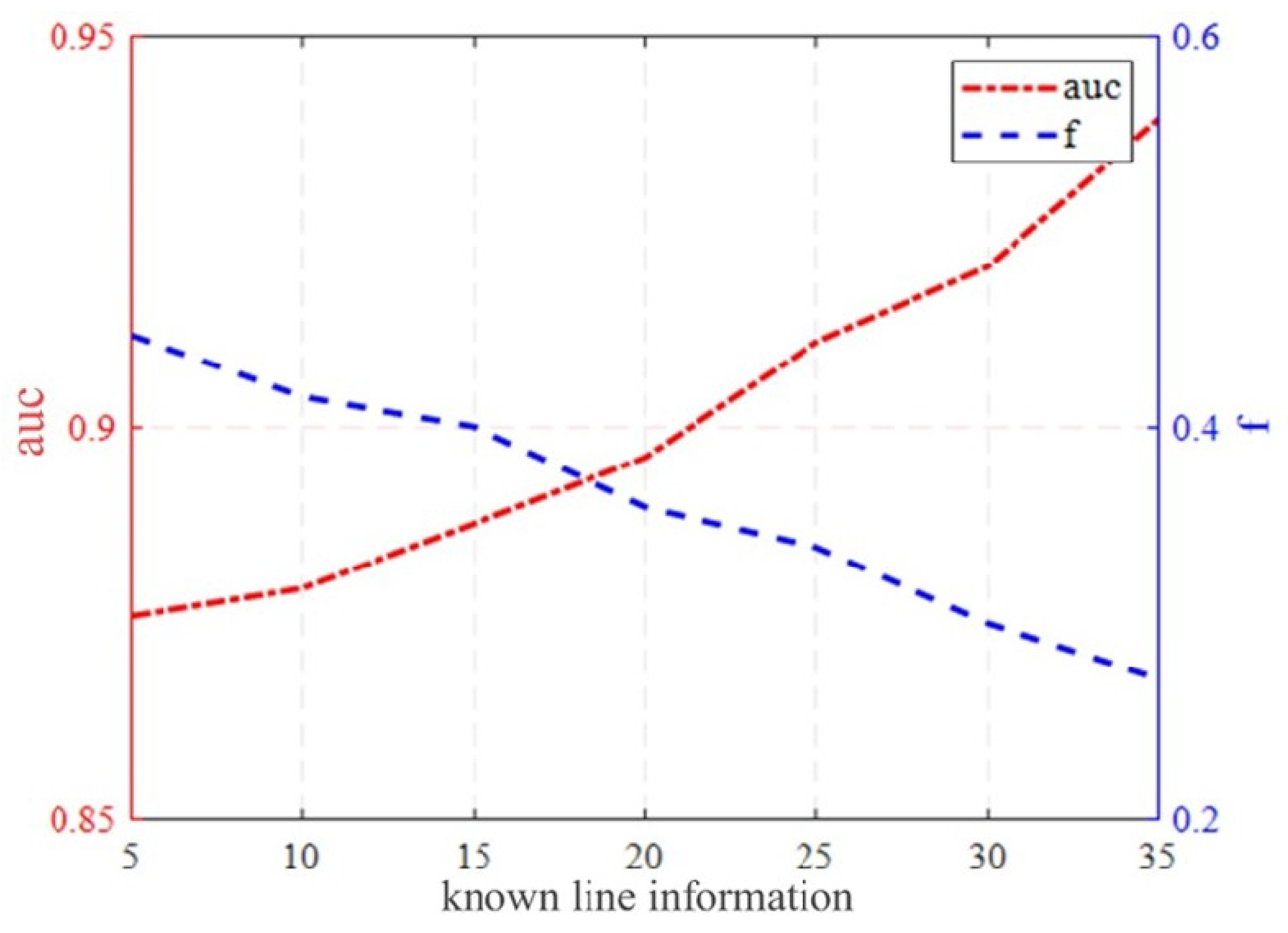
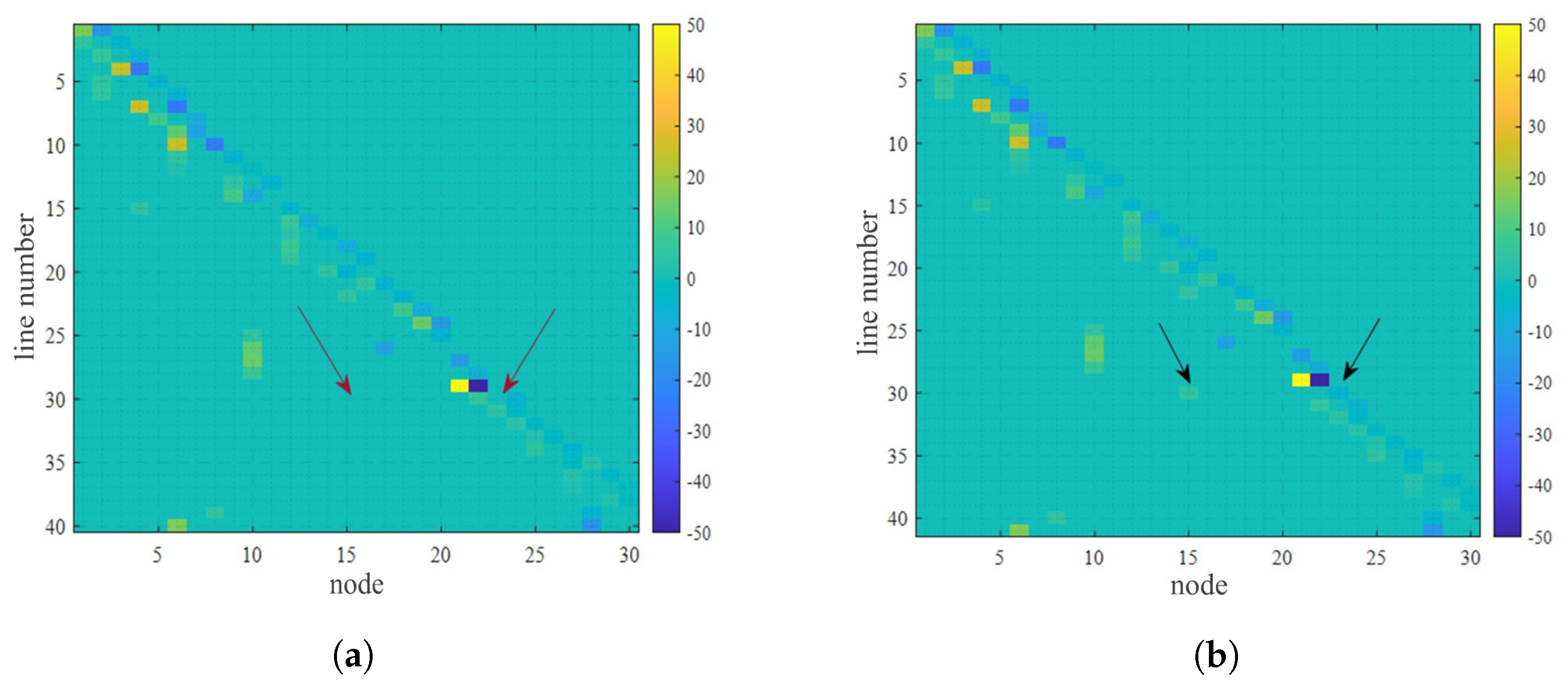
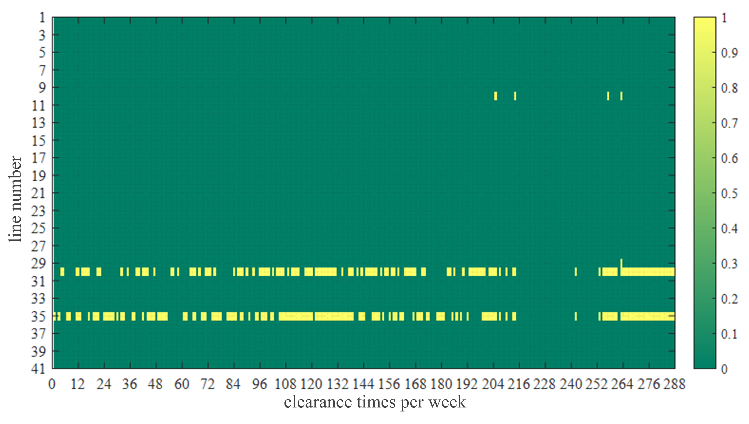
4.1. Performance Analysis of the System’s Topology Estimation

Firstly, we estimate the degree of damage done to the market test H ˜ 1 a c t ( L ˜ a c t ) in the IEEE 30-node system: in the case of D = , the estimated H ˜ 1 a c t and H ˜ a c t are compared with the corresponding real matrix, as shown in Figure 5 and Figure 6, respectively. As can be seen from the figure, although the estimated Jacobian matrix H ˜ a c t and the real matrix H have some similarities and differences in some values, the overall estimated effect is very good. The results show that FDI attacks only depend on the topology of the network, not on the concrete value of the matrix.
In order to analyze the accuracy of the estimated matrix more objectively, we analyze the estimated matrix according to the proposed performance index. Firstly, the AUC-ROC curve for the case of D = was calculated. It can be seen from Figure 7 that the AUC-ROC value is stable at about 0.86, which indicates that the estimation effect is good. However, to make the results more definitive, we plot the trend of accuracy in the loss market as the VB owns line information, as shown in Figure 8. With the increase in the known circuit information, the OC-ROC value gradually increases. At the highest value, it can reach about 0.94, while the F value gradually decreases. The lowest value it can reach is about 0.27. This shows that the estimation performance of H ˜ a c t improves with the increase in line information obtained by the VB.
Secondly, we propose an algorithm for restoring the topology online; that is, the current H ˜ a c t estimate can be updated immediately whenever the latest LMP is published. To prove that the proposed model can estimate the current topology, we conduct an additional case study to simulate the tracking of topological changes. As shown in Figure 9, Figure 9a is the K ˜ a c t estimated iteratively before the system’s topology changes, and Figure 9b is the K ˜ a c t estimated by the last iteration after the system’s topology changes. By comparing Figure 9a,b, it can be seen that, at line 30, the connecting nodes 15 and 23 are cut off, and the estimation model has a high level of accuracy for the change, which indicates that the topology can be estimated online in real time.
In addition, because the VB can obtain the market price data, the congestion in a certain segment of the market can be obtained by processing the congestion price. As shown in Figure 10, taking the market data from one week as an example, it can be known from the proposed strategy that congestion often occurs on lines 30 and 35 in many periods, and congestion occurs on line 10 in some periods, which provides great help for subsequent attacks.

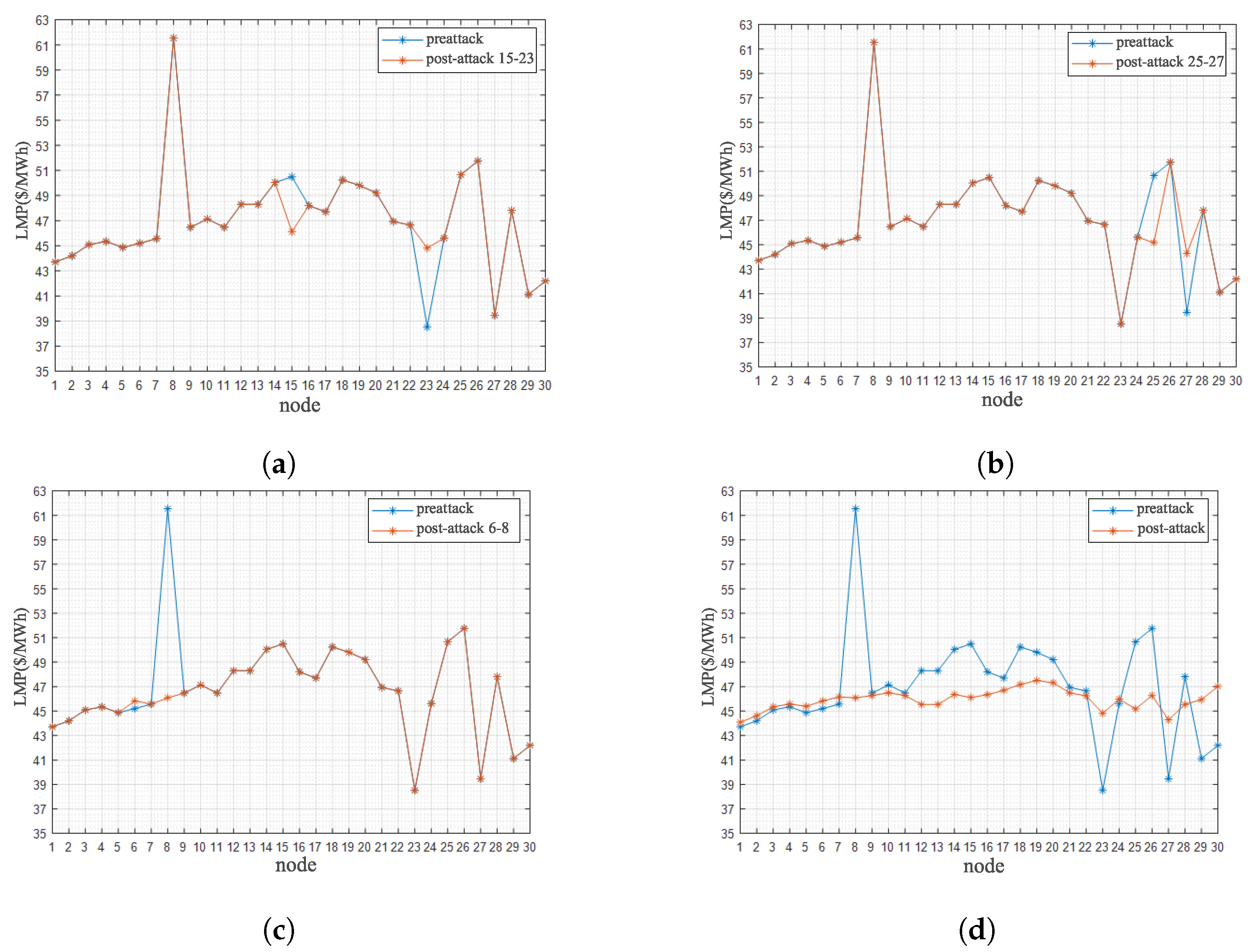
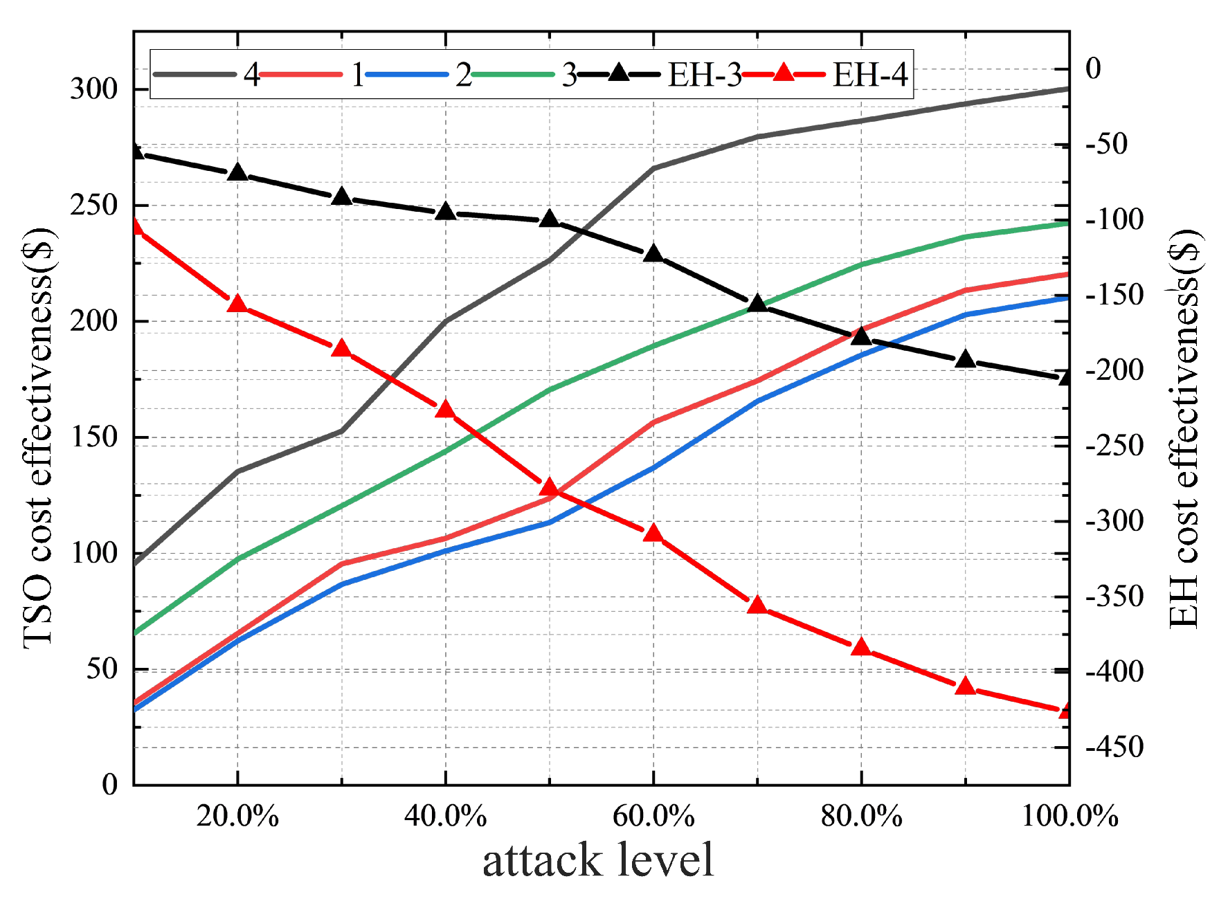
4.2. Economic Analysis under False Data Injection Attacks

Firstly, the transfer entropy between the LMP and VB objective function U is calculated based on the causality inference of the MTE. Then, on this basis, the contribution values of the LMPs of different nodes to the profit function are calculated, and the node variables that contribute more to the profit function at this moment are screened out according to the calculated screening standard value, and then the recognition result graph between variables based on the contribution rate of transfer entropy is obtained.
Figure 11 shows the contribution of each variable in a certain period and the contribution of the LMP of each node to the objective function U can be clearly seen. It is obvious that variables 8, 15, and 24 contribute more at this time and have high levels of impact on the generation of VB profits. At this point, the attacker gains the most, and the adverse impact on the energy market is greater.
In order to more clearly see the impact of the attacked section on other nodes, connected lines, and the attacker’s objective function, a heat map of the impact of the attacker on the price in the IEEE 30 bus network is drawn, as shown in Figure 12. It can be seen from Figure 12b that when an attack is launched on eight nodes (EH3), nodes 6 and 8 are the most affected. Figure 12c shows that the attack on 15 nodes has the greatest impact on nodes 14 (EH4), 12 (EH1), 18, and 23. Figure 12d shows that when an attack is launched against 24 nodes, nodes 22, 23, and 25 have the greatest impacts. After a comparison, the attacker in Figure 12b has the highest profit, followed by the result shown in Figure 12c, so the attacker can preferentially choose the attack mode, as shown in Figure 12b. According to the estimation method presented in Section 3.3, the congestion lines occur at lines 10, 30, and 35, among which line 30 is just connected to nodes 15 and 23, indicating that the two-stage attack can achieve a good target selection and attack effect.
The attacker first selects nodes 15 and 23 and line 30 as the attack set; second, it selects nodes 25 and 27 and line 35 as the attack set; and third, it selects nodes 8 (EH3) and 6 and line 10 as the attack set. The DA and RT virtual bidding (VB) information according to the four attack schemes is shown in Table 2.
Firstly, we combine the line congestion analyzed in Section 4.1 and select the 257th clearing price in Figure 13 for the attack. Then, according to the attack set obtained by the proposed method, the fourth one is selected as the attack set combination according to Table 2. The LMP before and after the attack of each node in Figure 14 can be obtained, and the profit of the VB can be calculated. Through the VB profit comparison under each scheme, it can be seen that the fourth attack set has the best effect and the biggest profit.
Finally, the effect of the above attack scheme on the income of TE market players is analyzed. Figure 15 compares the impacts of different attack schemes on the TSO cost and EH cost under different attack degrees. A higher attack degree means that the executed attack has a higher penetration level for congestion elimination. With the increase in the attack level under different attack schemes, the change in the TSO cost is constantly increasing. Option 4 is more cost-effective than other options. This is because scenario 4 causes the LMP of multiple nodes, resulting in reduced revenue from sales and increased flexibility costs.

5. Conclusions

The research focuses on developing a price-oriented TE market clearing model that emphasizes market security. The model takes into account coordinated transactions among the TSO, GMO, and EHs. To overcome the limitations of existing attacks, a two-stage attack strategy was proposed. In the first stage, a real-time topology estimation method driven by market data is devised to lay the groundwork for subsequent successful FDI attacks. In the second stage, the attacker’s role is determined based on the feasible attack modes within the TE market environment. Furthermore, an objective function for the attacker from a profit perspective was proposed. In addition, the authors introduced an optimal attack target identification method based on the MET to maximize the attacker’s profit while minimizing the risk. Lastly, an extensive simulation analysis was used to validate the effectiveness of the proposed attack strategy, which is essential for ensuring the security, stability, and effectiveness of the TE market.

Author Contributions

Validation, Z.S.; Writing—original draft, J.T.; Writing—review & editing, B.H., L.L., L.F. and G.J. All authors have read and agreed to the published version of the manuscript.

Funding

National Natural Science Foundation of China under grants (52377079); Liaoning Revitalization Talents Program under grant (XLYC2007181).

Data Availability Statement

The data presented in this study are available on request from the corresponding author.

Conflicts of Interest

Author Zewen Shi was employed by the Zhangjiakou Power Supply Company of Jibei Electric Power Company Limited. The remaining authors declare that the research was conducted in the absence of any commercial or financial relationships that could be construed as a potential conflict of interest.

References

  1. Favre-Perrod, P. A vision of future energy networks. In Proceedings of the 2005 IEEE Power Engineering Society Inaugural Conference and Exposition in Africa, Durban, South Africa, 11–15 July 2005; pp. 13–17. [Google Scholar]
  2. Esmalifalak, M.; Nguyen, H.; Zheng, R.; Xie, L.; Song, L.; Han, Z. A Stealthy Attack Against Electricity Market Using Independent Component Analysis. IEEE Syst. J. 2018, 12, 297–307. [Google Scholar] [CrossRef]
  3. Azizan Ruhi, N.; Dvijotham, K.; Chen, N.; Wierman, A. Opportunities for Price Manipulation by Aggregators in Electricity Markets. IEEE Trans. Smart Grid 2018, 9, 5687–5698. [Google Scholar] [CrossRef]
  4. Li, T.; Huang, R.; Chen, L.; Jensen, C.S.; Pedersen, T.B. Compression of Uncertain Trajectories in Road Networks. In Proceedings of the 46th International Conference on Very Large Data Bases, Online, 31 August–4 September 2020; pp. 1050–1063. [Google Scholar]
  5. Teng, F.; Zhang, Y.; Yang, T.; Li, T.; Xiao, Y.; Li, Y. Distributed Optimal Energy Management for We-Energy Considering Operation Security. IEEE Trans. Netw. Sci. Eng. 2023. [Google Scholar] [CrossRef]
  6. Li, Y.; Gao, D.W.; Gao, W.; Zhang, H.; Zhou, J. Double-Mode Energy Management for Multi-Energy System via Distributed Dynamic Event-Triggered Newton-Raphson Algorithm. IEEE Trans. Smart Grid 2020, 11, 5339–5356. [Google Scholar] [CrossRef]
  7. Li, Y.; Gao, D.W.; Gao, W.; Zhang, H.; Zhou, J. A Distributed Double-Newton Descent Algorithm for Cooperative Energy Management of Multiple Energy Bodies in Energy Internet. IEEE Trans. Ind. Inform. 2021, 17, 5993–6003. [Google Scholar] [CrossRef]
  8. Huang, B.; Li, Y.; Zhan, F.; Sun, Q.; Zhang, H. A Distributed Robust Economic Dispatch Strategy for Integrated Energy System Considering Cyber-Attacks. IEEE Trans. Ind. Inform. 2022, 18, 880–890. [Google Scholar] [CrossRef]
  9. Huang, B.; Liu, L.; Zhang, H.; Li, Y.; Sun, Q. Distributed Optimal Economic Dispatch for Microgrids Considering Communication Delays. IEEE Trans. Syst. Man Cybern. 2019, 49, 1634–1642. [Google Scholar] [CrossRef]
  10. Shekari, T.; Gholami, A.; Aminifar, F. Optimal energy management in multi-carrier microgrids: An MILP approach. J. Mod. Power Syst. Clean Energy 2019, 7, 876–886. [Google Scholar] [CrossRef]
  11. Liu, Z.; Huang, B.; Hu, X.; Du, P.; Sun, Q. Blockchain-Based Renewable Energy Trading Using Information Entropy Theory. IEEE Trans. Netw. Sci. Eng. 2023. [Google Scholar] [CrossRef]
  12. Liu, Z.; Xu, Y.; Zhang, C.; Elahi, H.; Zhou, X. A blockchain-based trustworthy collaborative power trading scheme for 5G-enabled social internet of vehicles. Digit. Commun. Netw. 2022, 8, 976–983. [Google Scholar] [CrossRef]
  13. Chen, Y.; Wei, W.; Liu, F.; Wu, Q.; Mei, S. Analyzing and validating the economic efficiency of managing a cluster of energy hubs in multi-carrier energy systems. Appl. Energy 2018, 230, 403–416. [Google Scholar] [CrossRef]
  14. Zhang, N.; Sun, Q.; Yang, L.; Li, Y. Event-Triggered Distributed Hybrid Control Scheme for the Integrated Energy System. IEEE Trans. Ind. Inform. 2022, 18, 835–846. [Google Scholar] [CrossRef]
  15. Yang, Z.; Hu, J.; Ai, X.; Wu, J.; Yang, G. Transactive Energy Supported Economic Operation for Multi-Energy Complementary Microgrids. IEEE Trans. Smart Grid 2021, 12, 4–17. [Google Scholar] [CrossRef]
  16. Najafi, A.; Falaghi, H.; Contreras, J.; Ramezani, M. A Stochastic Bilevel Model for the Energy Hub Manager Problem. IEEE Trans. Smart Grid 2017, 8, 2394–2404. [Google Scholar] [CrossRef]
  17. Sheikhi, A.; Rayati, M.; Bahrami, S.; Mohammad Ranjbar, A. Integrated Demand Side Management Game in Smart Energy Hubs. IEEE Trans. Smart Grid 2015, 6, 675–683. [Google Scholar] [CrossRef]
  18. Kamyab, F.; Bahrami, S. Efficient operation of energy hubs in time-of-use and dynamic pricing electricity markets. Energy 2016, 106, 343–355. [Google Scholar] [CrossRef]
  19. Cintuglu, M.H.; Martin, H.; Mohammed, O.A. Real-Time Implementation of Multiagent-Based Game Theory Reverse Auction Model for Microgrid Market Operation. IEEE Trans. Smart Grid 2015, 6, 1064–1072. [Google Scholar] [CrossRef]
  20. Azar, A.G.; Nazaripouya, H.; Khaki, B.; Chu, C.-C.; Gadh, R.; Jacobsen, R.H. A Non-Cooperative Framework for Coordinating a Neighborhood of Distributed Prosumers. IEEE Trans. Ind. Inform. 2019, 15, 2523–2534. [Google Scholar] [CrossRef]
  21. Luo, F.; Dong, Z.Y.; Liang, G.; Murata, J.; Xu, Z. A Distributed Electricity Trading System in Active Distribution Networks Based on Multi-Agent Coalition and Blockchain. IEEE Trans. Power Syst. 2019, 34, 4097–4108. [Google Scholar] [CrossRef]
  22. Papalexopoulos, A.; Beal, J.; Florek, J.S. Precise Mass-Market Energy Demand Management Through Stochastic Distributed Computing. IEEE Trans. Smart Grid 2013, 4, 2017–2027. [Google Scholar] [CrossRef]
  23. Li, R.; Wei, W.; Mei, S.; Hu, Q.; Wu, Q. Participation of an energy hub in electricity and heat distribution markets: An MPEC approach. IEEE Trans. Smart Grid 2019, 10, 3641–3653. [Google Scholar] [CrossRef]
  24. Mohamed, M.A.; Tajik, E.; Awwad, E.M.; El-Sherbeeny, A.M.; Elmeligy, M.A.; Ali, Z.M. A two-stage stochastic framework for effective management of multiple energy carriers. Energy 2020, 8, 117–170. [Google Scholar] [CrossRef]
  25. Xie, L.; Mo, Y.; Sinopoli, J.B. Integrity Data Attacks in Power Market Operations. IEEE Trans. Smart Grid 2011, 2, 659–666. [Google Scholar] [CrossRef]
  26. Deng, R.; Xiao, G.; Lu, R.; Liang, H.; Vasilakos, A.V. False Data Injection on State Estimation in Power Systems—Attacks, Impacts, and Defense: A Survey. IEEE Trans. Ind. Inform. 2017, 13, 411–423. [Google Scholar] [CrossRef]
  27. Zhang, Q.; Li, F.; Shi, Q.; Tomsovic, K.; Sun, J.; Ren, L. Profit-Oriented False Data Injection on Electricity Market: Reviews, Analyses, and Insights. IEEE Trans. Ind. Inform. 2021, 17, 5876–5886. [Google Scholar] [CrossRef]
  28. Kekatos, V.; Giannakis, G.B.; Baldick, R. Online Energy Price Matrix Factorization for Power Grid Topology Tracking. IEEE Trans. Smart Grid 2016, 7, 1239–1248. [Google Scholar] [CrossRef]
  29. Li, Y.; Zhang, H.; Liang, X.; Huang, B. Event-Triggered-Based Distributed Cooperative Energy Management for Multienergy Systems. IEEE Trans. Ind. Inform. 2019, 15, 2008–2022. [Google Scholar] [CrossRef]
  30. Rahman, M.A.; Venayagamoorthy, G.K. A Survey on the Effects of False Data Injection Attack on Energy Market. In Proceedings of the 2018 Clemson University Power Systems Conference (PSC), Charleston, SC, USA, 4–7 September 2018; pp. 1–6. [Google Scholar]
  31. Moslemi, R.; Mesbahi, A.; Mohammadpour Velni, J. Design of robust profitable false data injection attacks in multi-settlement electricity markets. IET Gener. Transm. Distrib. 2018, 12, 1263–1270. [Google Scholar]
  32. Choi, D.-H.; Xie, L. Sensitivity Analysis of Real-Time Locational Marginal Price to SCADA Sensor Data Corruption. IEEE Trans. Power Syst. 2014, 29, 1110–1120. [Google Scholar] [CrossRef]
  33. Choi, D.-H.; Xie, L. Impact of power system network topology errors on real-time locational marginal price. J. Mod. Power Syst. Clean Energy 2017, 5, 797–809. [Google Scholar] [CrossRef]
  34. Li, T.; Chen, L.; Jensen, C.S.; Pedersen, T.B.; Gao, Y.; Hu, J. Evolutionary Clustering of Moving Objects. In Proceedings of the IEEE 38th International Conference on Data Engineering Workshops (ICDEW), Kuala Lumpur, Malaysia, 9 May 2022; pp. 2399–2411. [Google Scholar]
  35. Mengis, M.R.; Tajer, A. Data Injection Attacks on Electricity Markets by Limited Adversaries: Worst-Case Robustness. IEEE Trans. Smart Grid 2018, 9, 5710–5720. [Google Scholar] [CrossRef]
  36. Tan, S.; Song, W.-Z.; Stewart, M.; Yang, J.; Tong, L. Online Data Integrity Attacks Against Real-Time Electrical Market in Smart Grid. IEEE Trans. Smart Grid 2018, 9, 313–322. [Google Scholar] [CrossRef]
  37. Yu, S.; Alesiani, F.; Yu, X.; Jenssen, R.; Principe, J.C. Measuring dependence with matrix-based entropy functional. Proc. AAAI Conf. Artif. Intell. 2021, 35, 12. [Google Scholar] [CrossRef]
Figure 1. The node’s local energy community structure.
Mathematics 11 04728 g001
Figure 2. The attacker’s role in the TE market. (a) The communication channel of the FDI attack. (b) Malicious users of FDI attacks.
Mathematics 11 04728 g002
Figure 3. The learning and execution phase of a data-driven FDI attack.
Mathematics 11 04728 g003
Figure 4. The node’s local energy community structure.
Mathematics 11 04728 g004
Figure 5. The node’s admittance matrix estimation: (a) real H 1 ; (b) estimated H ˜ 1 a c t .
Mathematics 11 04728 g005
Figure 6. Jacobian matrix estimation: (a) real H; (b) estimated H ˜ a c t .
Mathematics 11 04728 g006
Figure 7. AUC-ROC without line information.
Mathematics 11 04728 g007
Figure 8. AUC-ROC with line information.
Mathematics 11 04728 g008
Figure 9. Before and after the topology change: (a) before the topology change; (b) after the topology change.
Mathematics 11 04728 g009
Figure 10. Line congestion within a week.
Mathematics 11 04728 g010
Figure 11. The contribution of each node.
Mathematics 11 04728 g011
Figure 12. Causal graph between the variables before and after the attack. (a) Causal graph between the variables before the attack. (b) Causal graph between the variables after attacking eight nodes. (c) Causal graph between the variables after attacking 15 nodes. (d) Causal graph between the variables after attacking 24 nodes.
Mathematics 11 04728 g012
Figure 13. Line congestion for the 257th time.
Mathematics 11 04728 g013
Figure 14. LMP changes in the nodes before and after the attacks. (a) The LMP of nodes 15–23 before and after the attack. (b) The LMP of nodes 25–27 before and after the attack. (c) The LMP of nodes 6–8 before and after the attack. (d) The LMP of nodes before and after the attack.
Mathematics 11 04728 g014
Figure 15. Analysis of the effects of different attack schemes.
Mathematics 11 04728 g015
Table 1. Virtual bid trading scheme.
Virtual Bid NodeNode i (DA)Node j (DA)Node i (RT)Node j (RT)
Electricity Sold P d , M W - π j , L M P D A π i , L M P R T -
Electricity Purchase P d , M W π i , L M P D A -- π j , L M P R T
Table 2. Information for the attack schemes.
Attack SelectionVB1VB2Target LineAttacker Profit
Attack set 11523301003.67
Attack set 2252735966.084
Attack set 38 (EB3)6101544.17
Attack set 48 (EB3)2310/30/352111.31
Disclaimer/Publisher’s Note: The statements, opinions and data contained in all publications are solely those of the individual author(s) and contributor(s) and not of MDPI and/or the editor(s). MDPI and/or the editor(s) disclaim responsibility for any injury to people or property resulting from any ideas, methods, instructions or products referred to in the content.

