Article

Integrating a Pareto-Distributed Scale into the Mixed Logit Model: A Mathematical Concept

1
Department of Economics on Sustainability, Faculty of Economics, Dokkyo University, 1-1, Gakuen-cho, Soka-shi 340-0042, Saitama, Japan
2
Graduate School of Global Humanities and Social Sciences, Nagasaki University, 1-14, Bunkyo-machi, Nagasaki-shi 852-8521, Nagasaki, Japan
*
Author to whom correspondence should be addressed.
Mathematics 2023, 11(23), 4727; https://doi.org/10.3390/math11234727
Submission received: 31 October 2023 / Revised: 18 November 2023 / Accepted: 20 November 2023 / Published: 22 November 2023

Abstract

:
A generalized multinomial logit (G-MNL) model is proposed to alleviate the four challenges inherent to the conditional logit model, including (1) simultaneous unidentifiability, (2) the immediacy of decision-making, (3) the homogeneity of preferences in unobservable variables, and (4) the independence of irrelevant alternatives. However, the G-MNL model has some restrictions that are caused by the assumed logit scale of the lognormal distribution used in the G-MNL model. We propose a mixed logit with integrated Pareto-distributed scale (MIXL-iPS) model to address the restriction of the G-MNL model by introducing a logit scale in accordance with the Pareto distribution type I with an expected value of 1. We have clarified the mathematical properties and examined the distributional properties of the novel MIXL-iPS model. The results suggest that the MIXL-iPS model is a model in which the instability in the estimation of the G-MNL model is modified. Moreover, the apparent preference parameter was confirmed to have a skewed distribution in general in the MIXL-iPS model. In addition, we confirm that in the MIXL-iPS model, bounded rationality is reasonably well represented, as many individuals have below-average choice consistency.

1. Introduction

The conditional logit (CL) model is the gold standard in the social sciences’ axiomatic understanding of choice behavior. According to McFadden [1] and Yellot [2], only the CL model is compatible with all of the utility maximization requirements of microeconomics, the Choice Axiom [3], and the Law of Comparative Judgment [4]. The CL model is the basis not only for numerous case studies in policy evaluation and marketing but also for a quantal response equilibrium or a logit equilibrium model in experimental economics [5], which are expected to lead to an understanding of bounded rational human behavior [6]. The drift-diffusion model [7], which is the primary model used for response time analysis in cognitive psychology, also derives its most basic structure from the form of the CL model [8,9]. Even as descriptive response-time analysis models are being developed and case studies are accumulating in cognitive psychology, the need to consider CL extensions aligned with the tradition of axiomatic understanding in psychological research is being discussed [10]. Thus, the CL model is expected to continue to play a broad role in the social sciences in general.
Data collected through discrete choice experiments (DCEs) or choice-based conjoint analysis have played an essential role in the application and extension of the CL model [11,12,13]. DCE data were used to extend the CL model by accumulating empirical examples through the examination of a wide range of models, from closed-form to open-form and from continuous to discrete distributions regarding the probability distributions assumed for the preference parameters. DCEs have excellent characteristics in question design, data collection, and estimation. First, regarding question design, the use of DCEs can ensure statistical efficiency while avoiding multicollinearity among attribute variables within choice sets by using excellent experimental design methods [12]. Second, regarding data collection, the use of survey research data has the advantage of enabling various covariates to be obtained, making it easy to examine the validity of the application of the CL model and its extensions. In recent years, since Meißner and Decker [14], the number of examples of eye-tracking experiments, including among DCEs, has increased, and the use of more para data in the study of modeling has accelerated. Third, regarding estimation, in advanced methods such as simulated maximum likelihood estimation and hierarchical Bayes estimation [13], DCE data occupy a pivotal position in research aimed at more appropriate CL extensions.
The mixed logit (MIXL) model [15] was a central extension of the CL model. The MIXL model is also called the random parameter logit model [13]. The MIXL model is an open-form econometric discrete choice model that maintains the structure of the axiomatic understanding of the CL model while also having the flexible error structure of the conditional probit model [16]. The MIXL model can approximate any discrete choice model that is consistent only with random utility [17], and the number of applications continues to increase. The MIXL model is also at the center of the discussion in this paper.
From a review of previous studies on CL extensions, the authors identified four characteristics of the CL model that require resolution: (1) simultaneous unidentifiability: the CL model cannot be used to simultaneously identify true preferences and logit scale; (2) the immediacy of decision-making: the CL model cannot be used to account for the effects of sequential information sampling and processing; (3) the homogeneity of preferences in unobservable variables: the CL model is difficult to use for analyzing unobservable preference heterogeneity; and (4) the independence of irrelevant alternatives (IIA): the CL model cannot be used to account for the heterogeneous effects of additional alternatives. We note that, because multiple scale parameters appear in this paper, they are denoted as explicit model or distribution names, like logit scale. All of these characteristics stem from the assumption of independent and identical Gumbel error terms. Primarily, (1)–(4) are the crucial issues in the CL model. While (3) and (4) have been resolved in an econometric sense in the MIXL model, (1) is still being explored [18]. Moreover, when (1) is mitigated, (2) is also mitigated [9].
Fiebig et al. [19] developed a generalized multinomial logit (G-MNL) model, which was once regarded as an extended MIXL model that could also apparently resolve issues (1) and (2) [19,20]. However, Hess and Train [18] pointed out that it is the restricted form of the MIXL model. On the other hand, Ohdoko [21], one of the authors of this paper, conducted an empirical study of the G-MNL model using Japanese undergraduate survey data on a takeaway cup of fair trade coffee. The results suggest that the G-MNL model may be inferior to MIXL regarding model fit. The results of Ohdoko [21] are one of the motivations for the research in this paper.
Inspired by Adamska et al. [22], who examined the distribution of the product of the lognormal or normal distribution and the Pareto distribution, we propose the integration of a Pareto-distributed scale that can appropriately mitigate (1)–(4) of the CL issues and has behaviorally reasonable interpretability into the MIXL model. We refer to it as a mixed logit with integrated Pareto-distributed scale (MIXL-iPS). The basic structure of the MIXL-iPS model assumes a normal or lognormal distribution for the true preference parameter and a Pareto distribution type I [23] with expectation 1 for the logit scale. It has the property of being able to produce behaviorally reasonable results from a broad dataset. Rezapour and Ksaibati [24], who applied the G-MNL model to DCE data on front-seat passengers’ choice of seat belt usage, reported no need to introduce scale heterogeneity in their dataset. However, the conclusion may or may not change if the assumption of the distribution function of the logit scale changes.
The remainder of this paper is structured as follows. In Section 2, as a review of previous studies, we first confirm the derivation of the CL model and summarize its issues, and then, we present our research question. In Section 3, the MIXL model is discussed as an open-form model aimed at resolving issues (3) and (4) of the CL model, and we introduce the G-MNL model as the base model in this paper. In Section 4, we propose a basic MIXL-iPS model for a single-choice opportunity and perform numerical simulations of the parameter properties. Section 5 presents conclusions and future work. Some of the elementary mathematical derivations and analytical considerations performed in previous studies are also described in the discussion for clarity. In this paper, we present theoretical evidence of the ability of datasets to be used to validate the model properties of the MIXL-iPS model. One idea for future empirical research is the use of eye-tracking experiments.

2. The Conditional Logit Model

2.1. Derivations and Challenges

In this paper, a single choice opportunity is assumed, except when necessary. The notation common throughout the description is as follows: n n = 1 , 2 , , N denotes an individual, i i = 1 , 2 , , J is the chosen option, j j i , j = 1 , 2 , , J is the unchosen option, and k k = 1 , 2 , , K denotes the type of choice attribute. N denotes the sample size, J is the total number of choices in the choice set, and K is the total number of attributes in a choice set. When we use j * , i and j i are covered. Let the true preference parameter be α , the logit scale be φ , and their product, the apparent preference parameter β = α φ . As exogenous variables, the choice attributes and the covariates are denoted by x and z , respectively. The Dirac delta function is represented by δ for the probability density function f and the cumulative distribution function F , respectively. Although developed with DCE data in mind, our approach readily applies to other choice situations and should be read by the reader as appropriate.
In deriving the CL model, the additive random utility model (ARUM), which we also assume in this paper, is defined as follows [13]:
U i = V i + ε i
U i is the indirect utility of chosen alternative i . V i is an observable deterministic term, and ε i is an unobservable error term.
McFadden [1] derived CL compatible with utility maximization in microeconomics by formulating the conditional choice probability as follows (see also Appendix A):
P i = P r o b U i > U j , j i
= e x p V i / ξ j e x p V j / ξ
Here, we assume that j J , ε j ˜ i . i . d . G u m b e l 0 , ξ , where ξ denotes the Gumbel scale. The probability density function and cumulative distribution function of the Gumbel distribution evaluated at the zero-location parameter are as follows:
f ε = 1 ξ e x p ε ξ e x p e x p ε ξ ,
F x = e x p e x p ε ξ ,   ξ > 0
where E ε = 0 and V a r ε = ξ 2 π 2 / 6 , respectively. ξ ; in situations where the variance of the error term or the Gumbel error is substantial, P j * 1 / J while the choices become indiscriminate. ξ 0 ; as the variance of the Gumbel error disappears, the choice becomes deterministic. Thus, the properties of the choice change with the magnitude of the impact of unobservable variables.
On the other hand, Marsili [25], through an analogy with the distribution of canonical ensembles or the Gibbs–Boltzmann distribution in thermodynamics and statistical physics, formulated the expected information processing cost of the choice task or DCE choice set faced by the decision maker in maximizing the expected utility using Shannon entropy [26] as follows [27].
max P i E [ U i ] = i P i V i + ξ i P i ln P i ,   s . t .   i P i = 1
The same choice probability as that in the CL model is derived here (see also Appendix B). ξ ; in situations where the overall expected cost of information processing is exceptionally high, every alternative becomes indifferent because P j * 1 / J . ξ 0 ; when the overall expected cost of information processing is minimal, the choice is made deterministically. Thus, the Gumbel scale assumed for the CL model expresses the marginal utility for the overall expected information processing cost of the choice set encountered. Marsili [25] designated its cost as the control cost. In this paper, we refer to it as a choice behavior control cost.
Here, as was assumed in previous DCE studies, we assume linearity concerning the true preference parameter in the definite term of the indirect utility function, as in V j * = α x j * k . From U i > U j in Equation (2), that is, α x i k + ε i > α x j k + ε j . If we multiply both sides by the logit scale φ = 1 / ξ > 0 , we obtain:
φ α x i + φ ε i > φ α x j + φ ε j
In this case, φ ε j * = ε j * / ξ = ε j * * ˜ i . i . d . G u m b e l 0 , 1 . Therefore, if U i * = φ U i , then the redefined linear-in-parameter ARUM becomes:
U i * = V i * + ε i * = φ α x i + ε i * = β x i + ε i * ,   ε i * ˜ i . i . d . G u m b e l 0 , 1
Therefore, the logit scale φ is multiplied by all elements in the linear-in-parameter ARUM except the Gumbel error [18].
The logit scale φ expresses the choice consistency [28]. The conditional choice probability, based on the redefined linear-in-parameter ARUM, becomes:
P i = P r o b U i * > U j * , j i
= P r o b ε j * ε i * < V i * V j * , j i
= P r o b ε j * ε i * < φ α x i α x j , j i
where ε j * ε i * follows a logistic distribution and the support is , . Thus, ε j * ε i * < φ α x i α x j is probabilistically valid as the logit scale increases with φ ; the larger the logit scale is, the higher the probability of choosing according to one’s true preference. Conversely, as φ 0 , the probability of choosing according to one’s true preference is reduced; the alternatives become indifferent such that P j * 1 / J .
At this stage, we can point out two of the challenges of using the CL model: (1) the simultaneous unidentifiability and (2) the immediacy of the decision-making as seen from the redefined linear-in-parameter ARUM; the logit scale and true preference parameters are estimated inseparably in the form of multiplication. Therefore, at least one expected value must be normalized to 1 to identify both the logit scale and the true preference parameters. If one wants to examine the true preference on a single dataset with the CL formulation, one has no choice but to normalize the logit scale expectation to 1 [29]. Webb [9] also showed in mathematical neuroeconomics that the CL model does not include the effects of dynamic and sequential information sampling and processing that can occur within a single-choice opportunity. In particular, the intuitive implications for the immediacy of the decision-making can be organized as follows. The heterogeneity of the logit scale is the heterogeneity of overall and cognitive choice behavior control costs. Since the logit scale is closely related to cognitive information processing, modeling the logit scale as constant across individuals or choice occasions, as CL does, implies that cognitive information processing is the same for any person or any choice occasion. Usually, cognitive information processing in choice behavior should differ from person to person or from choice opportunity to opportunity. Treating this as a constant would not be so much different from assuming that everyone makes all choices instantly at any time. To include them, one must introduce unobserved heterogeneity for the logit scale, i.e., scale heterogeneity. In DCE studies, the logit scale has also been correlated with response time [30] and survey engagement [31], suggesting the influence of dynamic and sequential information sampling and processing. Therefore, these challenges require a solution on the logit scale.
Traditional DCE research has indicated two issues with the CL model: (3) the homogeneity of preferences in unobservable variables and (4) the IIA [13]. It is possible to include the CL model with socioeconomic characteristics or para data in the analysis. Such data are used to express the deterministic heterogeneity in the analysis cross terms, the product with alternative attributes, or the alternative specific constants (ASCs), which can introduce up to J 1 alternatives [12]. However, we cannot consider the heterogeneity in unobservable variables. The ratio of the choice probabilities of the different alternatives, i and j j i , is as follows:
P i / P j = e x p V * i / e x p V * j
Therefore, the choices i and j are independent of the deterministic terms of the indirect utility functions of the alternatives other than i and j . This does not allow for nonuniform changes in choice probabilities when additional alternatives are introduced.

2.2. Research Question

In this paper, the research goal is to mathematically construct a discrete choice model that can appropriately relax the assumptions of (1) simultaneous unidentifiability, (2) the immediacy of decision-making, (3) the homogeneity of preferences in unobservable variables, and (4) the IIA, which can be considered the main aspects of the CL problem. We focus on the formulation of scale heterogeneity by using the logit scale.
We also consider the use of specifically open-form models that represent unobserved heterogeneity to enable the application of models to broad datasets. For logit scale formulation when using the covariate z n , the heteroskedastic multinomial logit model [11] with φ = e x p ϑ z n is omitted due to its inability to represent unobserved heterogeneity. When we need to set the distribution of the true preference parameters in the simulation, we assume a normal distribution for nonprice-related attributes and a lognormal distribution for price-related choice attributes in DCE questions. We chose the normal and lognormal distributions for the distribution of apparent preference parameters in this paper because the former is the most used in empirical studies, and the latter was recommended by Daly et al. [32] as a possible way to estimate the finite moments of the marginal willingness to pay (MWTP) by making assumptions about price-related attributes. Daly et al. [32] recommended that the finite moments of MWTP can be estimated by making assumptions on the apparent preference parameters of price-related attributes as log-normally distributed.

3. The Mixed Logit and the Generalized Multinomial Logit Models

3.1. The Mixed Logit Model and Its Challenges

The MIXL model relaxes (3) the homogeneity of preferences in unobservable variables by introducing unobserved heterogeneity in the apparent preference parameters. Here, let ASC be β 0 , and let the apparent preference parameters of the choice attributes be β k k = 1 , , K . When the apparent preference parameter vector β = β 0 , β 1 , , β K follows a multivariate probability distribution, the unconditional choice probability is formulated as follows:
P n i = e x p V * n i j * e x p V * n j * f β n d β n
The f β n have been assumed to be normal, lognormal, gamma, uniform, triangular, and Johnson Sb distributions [13,33]. It has also been shown that f β n can partially set apparent preference parameters without standard deviation or covariance, and in the MIXL model, such parameters are called fixed parameters, while apparent preference parameters other than fixed parameters are called random parameters [13]). In this paper, we use the following formulation in linear-in-parameter ARUM.
V * = β 0 + β p r i c e x p r i c e e x p β p r i c e x p r i c e .
The first term represents the ASCs, the second reflects the attribute terms related to the nonprice ( p r i c e ), and the third reflects the attribute terms related to the price ( p r i c e ). β n = β 0 , β n , p r i c e , β n , p r i c e ˜ N o r m a l μ β n , Σ β n ; then, e x p β n , p r i c e follows a (multivariate) lognormal distribution, where μ β n is the vector of expected values, and Σ β n is the covariance matrix of β n .
With the choice probability formulation, the MIXL model econometrically relaxes (4) the IIA. The ratio of the choice probabilities is:
j i ,   P n i / P n j = e x p V * n i j * e x p V * n j * f β n d β n / e x p V * n j j * e x p V * n j * f β n d β n
Closed-form solutions generally do not exist. Therefore, the IIA is entirely relaxed because the ratio of choice probabilities depends on the definite terms of the indirect utility functions of the alternatives other than i and j .
The apparent preference parameter vector β n allows for the correlations between elements, and Σ β n may include nonzero off-diagonal elements. For estimation, a Cholesky decomposition is used as in Σ β = Γ Γ . Then,
β n = μ β n + Γ v n , v = v n 0 , v n 1 , v n 2 , , v n K ,   v n k v n ˜ i . i . d . N o r m a l 0 , 1
This allows apparent preference heterogeneity [11,13].
In some previous studies, the MIXL model with correlation was modified when the MIXL model includes nonzero off-diagonal elements of Σ β n . According to Hess and Train [18], the MIXL model is a formulation that already allows correlations; thus, there is no need to specify a MIXL with correlation. However, since many original empirical papers assumed 0 for the covariance parameter, to be cautious, they are separately described here as the MIXL model and the MIXL model with correlation. Hess and Train [18] discussed that the correlation expresses behavioral phenomena and scale heterogeneity, where behavioral phenomenon is an interaction effect between true choice attribute preferences. Mariel and Artabe [34] gave a mathematical interpretation and provided the following three conditions under which the apparent preference covariance parameter can be interpreted: All the apparent preference parameters should be positively estimated; the interpretation is based on the negatively signed covariances only; and covariances should not be interpreted quantitatively.
From the above observations, the challenges of the MIXL model can be presented. Indeed, the MIXL model mitigates (3) the homogeneity of preferences in unobservable variables and (4) the IIA. McFadden and Train [17] proved that the MIXL model can approximate all discrete choice models that are consistent only with a random utility model. Therefore, extensions of the CL model should be discussed with a focus on the MIXL model. However, the implicit control of the logit scale does not allow for a quantitative examination of scale heterogeneity, and the use of covariance parameters for preferences is limited. In behavioral welfare economics, Grüne-Yanoff [35] suggested that it is necessary to distinguish welfare-related preferences from those that are not based on some notion of deliberation error. Moreover, because heterogeneity was incorporated into the apparent preferences, it cannot be construed as the true heterogeneity of preferences. The estimated parameters can be interpreted either (1) as the product of overall and cognitive choice behavior control costs and true preferences, (2) as true preferences with the logit scale for all individual and choice opportunities specified to be normalized to 1, or (3) as the monetary value of the preference, removing the effect of the logit scale by producing an MWTP value. The MWTP is estimated by dividing the apparent preference parameters for non-price-related attributes by the price-related parameters [11,12,13].

3.2. The Generalized Multinomial Logit Model and Its Challenges

Following the challenges of the MIXL model described in the previous section, the G-MNL model represents an attempt to explicitly alleviate (1) simultaneous unidentifiability. According to Webb [9], incidentally, (2) is also mitigating. The contribution of the G-MNL model is that the logit scale was given a distribution, and the observable individual characteristics were expressed as covariates to be incorporated into the mean and the unobservable portion as an error term [11]. Thus, unlike the MIXL model, the signs of the covariance parameters for all preference parameters are interpretable. β can be decomposed as follows [11].
β n = φ n α n + γ + 1 γ φ n Γ ˜ v ˜ n ,
φ n = exp μ φ n + τ w n ,   w n ˜ i . i . d . N o r m a l 0 , 1 ,   E φ n = 1 ,
α n ˜ N o r m a l μ α , Σ α , Σ α = Γ ˜ Γ ˜ ,
v n k v ˜ n = v 1 , v 2 , , v K ˜ i . i . d . N o r m a l 0 , 1 ,
γ 0 , 1
where μ φ n is the logit scale location parameter, τ is the lognormal scale, and φ n follows a lognormal distribution. Here, covariate z n effects on φ n can be included: In general, φ n = exp μ φ n + ϑ z n + τ w n . The section on covariates in Equation (13) was omitted in this paper to simplify the discussion. γ is a probability weight to define the following two types of G-MNL models in one equation:
G - M N L   t y p e   I : β n = φ n α n + Γ ˜ v ˜ n , γ = 1
G - M N L   t y p e   I I : β = φ n α n + φ n Γ ˜ v ˜ n , γ = 0
γ = exp γ * / 1 + exp γ * can be set to ensure the condition 0 < γ < 1 . Fiebig et al. [19] treated ASCs as fixed parameters in their empirical demonstrations, eliminating unobserved heterogeneity in the ASCs, although they incorporated random effects due to the panel structure of their DCE datasets. They also choose not to multiply the ASCs by the logit scale.
Since issue (1) of simultaneous unidentifiability cannot be completely mitigated due to the identification problem, in the estimation of the G-MNL model, n , E φ n = 1 . We note that in the G-MNL framework, the true preference parameter is always multiplied by the expected value of the logit scale. Therefore, we must inseparably treat the true preference parameter and the expected marginal utility value for the choice behavior control cost. From here, we can say that the logit scale in the G-MNL model is a mean-normalized relative logit scale. The implication is the degree to which each individual makes consistent choices relative to the average. From this perspective, in this paper, quantitative scale heterogeneity expressed by the logit scale in the G-MNL model is referred to as the relative consistency index.
At this stage, an issue with the G-MNL model can be identified. To reiterate the discussion regarding the redefinition of the linear-in-parameter ARUM in Section 2, the logit scale is multiplied by all factors in the linear-in-parameter ARUM aside from the Gumbel error [18]. Therefore, the G-MNL model type I is an unnatural extension of the CL model since the G-MNL model type I accounts for heterogeneity that is not explained by true choice attribute preferences in a way that is not multiplied by the logit scale, and the ASC is a fixed parameter, i.e., there is no unobserved heterogeneity in the ASC.
According to Hess and Train [18], the G-MNL model of Fiebig et al. [19] restricts the MIXL model. However, the G-MNL model type II can potentially improve the MIXL model because the MIXL model makes the probability distribution assumption only on the product of the true preference parameter and the logit scale parameter, eliminating the possibility that it may not be. Based on the G-MNL model type II, it is possible to relax the assumption of the MIXL model by assuming a tractable probability distribution for the logit scale. Therefore, our research focuses on the G-MNL model type II and examines the validity of a formulation that multiplies the ASCs by the logit scale; we treat all true preference parameters, including the ASCs, as random parameters.
In G-MNL estimation, a truncated normal distribution is used for w n [19,20]. The lack of a reasonable behavioral explanation for the truncated normal distribution suggests a technical issue in estimation stability. Therefore, we assume a normal distribution for the true preference defined in general G-MNL application studies and examine the product or multiplicative convolution of random variables with the logit scale according to a lognormal distribution with an expected value of 1. When we suppose that the true preference parameter is assumed to be lognormally distributed for price-related choice attributes, the apparent preference parameter is also lognormally distributed. Therefore, we omitted this case.
The apparent preference parameter is the multiplicative convolution of the logit scale and the true preference, where these are two continuous random variables that are statistically independent. Subscripts are omitted hereafter except when necessary. The probability density function can be expressed as follows, according to Rohatgi and Saleh [36].
f β β = 1 φ f φ φ f α β φ d φ
φ ˜ L o g n o r m a l μ φ , τ 2 ; then, the probability density function is defined as:
f φ φ = 1 2 π τ φ e x p l n φ μ φ 2 2 τ 2 ,   0 < φ <
The expected value is:
E φ = e x p μ φ + τ 2 2 .
The G-MNL assumption is E φ = 1 . Thus:
μ φ = τ 2 2 < 0 .
For the true preference parameter, α ˜ N o r m a l μ α , σ α 2 , the probability density function is:
f α α = 1 2 π σ α exp α μ α 2 2 σ α 2 , < α < .
By incorporating Equation (17) into (16) with (20), we obtain:
f β β = 1 2 π σ α τ 0 1 φ 2 e x p l n φ + τ 2 / 2 2 2 τ 2 β φ μ α 2 2 σ α 2 d φ .
No further closed-form solutions can be obtained. Thus, we performed simulations in R 4.2.1 [37] for illustration along with a simple algorithm diagram in Appendix C. In this paper, we use an elementary numerical simulation because the correlation of choice attribute variables and their true preference parameters can be complicated when multiple choice attributes are considered. Since the correlation of choice attribute variables can at least be set to zero in DCE data through an experimental design that preserves orthogonality, we consider it sufficient to examine the true preference parameters and logit scale parameters for a single choice attribute in this paper, which is mainly intended for use in DCE data. It is essential to examine what happens when multiple-choice attributes are considered, including misspecification, which is an issue to be addressed in the future.
In the numerical simulations, with emphasis on visibility in the illustrations, numerical examples were selected concerning empirical DCE studies. Before providing the numerical examples, we refer to Hess and Rose [38], who doubt the G-MNL model when using DCE data on route choice. First, they estimated by using the G-MNL model with correlation, assuming a bivariate normal distribution for the true preference parameter vector. The mean and standard deviation of the true preference parameters for travel time and travel cost were estimated as ( μ α ^ , σ α ^ ) = ( 0.1558 , 0.1991 ) , ( 0.4205 , 0.1412 ) . The standard deviation of the logit scale with the expected value of 1 is τ ^ = 2.0843 The estimated standard deviations of the logit scale with an expected value of 1 were obtained. Next, assuming a bivariate lognormal distribution for the true preference parameter vector, they obtained ( μ α ^ , σ α ^ ) = ( 1.7353 , 1.9004 ) , ( 0.9238 , 1.5296 ) for the travel time and travel cost, respectively, and τ ^ = 0.1169 for the logit scale. For visibility and simplicity, absolute values were taken for the parameters under the assumption of a normal distribution and for the standard deviation of the logit scale of an expected value of 1, while the travel time was omitted. The same simulation results were obtained by using the travel time parameter.
When conducting the numerical simulation, the R package distrSim [39] was used to run the simulations. In the simulations, given that the G-MNL estimation uses a truncated normal distribution to limit the variance of the logit scale, we decided to investigate the impact of τ in the G-MNL model. We also decided to include simulation results by using the estimate of τ in Hess and Rose [38] to ensure realism. For illustrative purposes, we set a relatively wide range of values in the defined region of τ around the mean estimated value of Hess and Rose [38] when the logit scale depends on lognormal distribution. The robustness of the results at the analytical limit values was elaborated in Appendix D.
The simulation results are shown in Figure 1. As τ 0 (from Figure 1c to Figure 1a), the apparent preference parameter distribution converges to the normal distribution set for the true preference parameter. On the other hand, as τ (from Figure 1d to Figure 1f), the distribution loses its significance after converging to a point in the parameter domain of 0 through a distribution with high kurtosis. Because of mathematical properties of the assumption of logit scale as lognormally distributed in Appendix D, these properties hold for general continuous probability distributions with moments, rather than only when the true preference parameter is normally or lognormally distributed.
This brings us to another issue of the G-MNL model. As the variance of the logit scale decreases, the apparent preference parameter distribution comes to match the true preference parameter, which is a reasonable property. On the other hand, as the variance of the logit scale increases, the apparent preference parameter loses its meaning through distribution with a high kurtosis. This phenomenon results from the assumption of the lognormal distribution as set to the logit scale. Of course, it is possible that a situation of enormous variance on the logit scale does not occur in the actual data and that the use of a truncated normal distribution is reasonable. Assuming a lognormal distribution for the logit scale is also a reasonable interpretation since it corresponds to modeling in which more people have less consistent choices than in the average. In comparison, there are slightly fewer people faced with extremely inconsistent choices. However, the arbitrariness of the use of the lognormal distribution in the logit scale cannot be denied. There is also a question as to whether the possibility of higher kurtosis is a natural approximation. Thus, we can consider the possibility of applying other distributions to the logit scale.

4. Proposed Mixed Logit with Integrated Pareto-Distributed Scale Model

In this paper, we propose the MIXL-iPS model, the application of which can alleviate the issues described in the previous section. The apparent preference parameter of the MIXL-iPS model is defined as follows:
β n = φ n α n + φ n Γ v n ,
v = v n 0 , v n 1 , v n 2 , , v n K ,
v n k v n ˜ i . i . d . N o r m a l 0 , 1 ,
φ n ˜ P a r e t o κ , 1 / 1 κ , E φ n = 1 ,
1 / 2 < κ < 1
where κ is the Pareto scale of Pareto distribution type I with shape parameter 1 / 1 κ . The MIXL-iPS model is based on the G-MNL model type II, and the ASCs are also treated as random parameters multiplied by the logit scale. As described below, the assumption of a probability distribution for the logit scale ensures reasonable constraints both statistically and behaviorally.
As discussed in our assessment of the G-MNL model, we consider the multiplicative convolution of a mutually independent Pareto distribution type I and some continuous distribution. Let ζ be the shape parameter and φ ˜ P a r e t o κ , ζ , and let the probability density function and cumulative distribution function be [23]:
f φ φ = ζ κ ζ φ ζ + 1 = ζ κ φ / κ ζ + 1   i f   κ φ ,   0 < ζ 0   i f   0 φ < κ ,   0 < ζ ,  
F φ φ = 1 κ φ ζ   i f   κ φ ,   0 < ζ 0   i f   0 φ < κ ,   0 < ζ
The expected value and variance are:
E φ = ζ κ ζ 1 ζ > 1 ,
V a r φ = ζ κ 2 ζ 1 2 ζ 2 ζ > 2
Here, we normalized the expected value to 1 to obtain the MIXL-iPS model.
E φ = ζ κ ζ 1 = 1 .
In other words,
κ = ζ 1 ζ = 1 1 ζ ,   ζ = 1 1 κ
Therefore, to make sense of the variance, ζ > 2 , the constraint of κ becomes 1 / 2 < κ < 1 . The following sigmoid function can be used to ensure κ 1 / 2 , 1 :
κ = 1 1 + exp exp κ * ,   κ * , .
The constraints that 1 / 2 < κ < 1 of the MIXL-iPS model are highly behaviorally explainable. First, when ζ , κ 1 , and f φ φ δ φ 1 (see Appendix E for details). If we denote the probability density functions of α and β as f α α and f β β , respectively, then:
l i m ζ , κ 1 f β β = l i m ζ , κ 1 1 φ f φ φ f α β φ d φ
= l i m ζ , κ 1 1 φ ζ κ ζ φ ζ + 1 f α β φ d φ
= 0 δ φ 1 1 φ f α β φ d φ
= 1 1 f α β 1 ,
= f α β
Thus, the apparent preference parameter distribution of the MIXL-iPS model converges to the true preference parameter distribution. In other words, once the unobserved heterogeneity of the logit scale is lost, the distribution of the apparent preference parameter distribution always matches that of the true preference parameter. This property holds for general continuous probability distributions with moments, rather than only when the true preference parameter is normally or lognormally distributed. Moreover, because φ is a relative consistency index, it implicitly ensures that the range of the substantive logit scale will be 0 , rather than κ , ) .
In general, there is no closed-form solution for the probability density function of the product of the Pareto distribution type I and the normal or lognormal distribution. Therefore, numerical simulations were also performed here for illustrative purposes along with a simple algorithm diagram in Appendix C. The numerical example is based on Hess and Rose [38] and the G-MNL model as described in the previous section. For illustrative purposes, we set a relatively wide range of values in the defined region of κ when the logit scale depends on Pareto distribution type I. The robustness of the results at the analytical limit values was elaborated in Appendix E. The results corresponding to the assumption of a normal distribution for the true preference parameters are shown in Figure 2, and those corresponding to the assumption of a lognormal distribution are shown in Figure 3. In general, the result of multiplicative convolution is a skewed distribution. However, because Pareto distribution type I has the property of converging to Dirac’s delta function, the apparent preference parameter distribution converges to the true preference parameter distribution as the Pareto scale approaches 1. In other words, the apparent preference, which incorporates both true preference and scale heterogeneity with an expected value of 1, generally becomes a skewed distribution in the MIXL-iPS model framework. As the variance of the logit scale loses its significance, the true and apparent preference parameters converge. Finally, as a qualitative impression, judging from the graphs and compared with the results displayed in Figure 1, which were obtained from the G-MNL model, the kurtosis is not overly high in the results of multiple convolutions displayed in Figure 2 and Figure 3.
Finally, as the most extreme case, we examined how well the MIXL-iPS model can represent choice inconsistency. The cumulative distribution function of the Pareto distribution with expectation fixed at one becomes:
F φ φ = 1 κ φ 1 1 κ
When F φ φ is evaluated, the values up to E φ = 1 , then,
F φ 1 = 1 κ 1 1 1 κ = 1 κ 1 1 κ
Since 1 / 2 < κ < 1 ,
lim κ 1 2 1 κ 1 1 κ = 0.7500 ,   lim κ 1 1 κ 1 1 κ = 1.0000
Thus, the share that is below the expected value is between 0.7500 and 1.0000 . Thus, the MIXL-iPS model is an appropriate formulation of bounded rationality because many people are less consistent than in the average, and this is a model in which the share increases rapidly toward those who make extremely inconsistent choices.

5. Conclusions

In this paper, we proposed the MIXL-iPS model, which can be used to alleviate several significant issues inherent to the CL model, and we examine its parameter distribution properties. First, we summarized four issues inherent to the CL model: (1) simultaneous unidentifiability, (2) the immediacy of decision-making, (3) the homogeneity of preferences in unobservable variables, and (4) the IIA. Second, we discussed the limitations of the MIXL and G-MNL models. The former implicitly controls for the heterogeneity of the logit scale, which limits the use of covariance parameters and suggests that care must be taken in interpreting the estimated apparent preference parameters. For the latter, the assumption of a lognormal distribution for the logit scale suggests that the kurtosis of the distribution of the apparent preference parameters can be high when the variance is significant and that the estimation of the apparent preference parameters can fail when the variance is even more significant. Therefore, we constructed the MIXL-iPS model to address these issues. Third, we constructed a basic MIXL-iPS model that represents the situation with only one choice opportunity to resolve the restrictions of the MIXL and G-MNL models and to alleviate challenges (1) to (4) of the CL model. The basic MIXL-iPS model expresses the diversity of the relative consistency index for the choice set by introducing a logit scale according to the Pareto distribution type I with an expected value of 1 while also expressing the preference heterogeneity by assuming a normal or lognormal distribution for the true preference parameters. Numerical simulations confirm that the apparent preference parameters are generally skewed and become consistent with the true preference parameters as the variance implications of the logit scale disappear. Moreover, the kurtosis of the apparent preference parameter is not overly high in the MIXL-iPS model.
When estimating MIXL-iPS, the simulated maximum likelihood method developed by Train [13] for estimating MIXL and used by Fiebig et al. [19] for estimating G-MNL is promising. In addition to relatively small survey data, it was used to estimate MIXL on extensive consumer scanner data, as in Ankamah-Yeboah et al. [40], so we can expect it to be valid for a wide range of datasets. According to Fiebig et al. [19], in the estimating procedure of the simulated maximum likelihood method, the simulated choice probability takes the following form:
P i = 1 S s = 1 S e x p φ s α + φ s Γ v s x i j * e x p φ s α + φ s Γ v s x j *
where s s = 1 , 2 , , S denotes the number of pseudorandom variables drawn from v k s v s ˜ i . i . d . L o g n o r m a l 0 , 1 for price-related attributes, v k s v s ˜ i . i . d . N o r m a l 0 , 1 , for nonprice-related attributes, and for the logit scale, φ s ˜ P a r e t o κ s , 1 / 1 κ s where 1 / 2 < κ s < 1 .
It is necessary to empirically confirm the validity of the basic MIXL-iPS model and to compare it with the G-MNL model type II, which was modified to multiply the ASCs by the logit scale, and with the MIXL model, which considered the multiplicative distribution of true preference and the logit scale parameters assumed to be normal or lognormal. This is because there is no justification in behavioral theory for adopting a Pareto distribution on the logit scale a priori.
Then, it becomes necessary to consider how to resolve two relevant challenges, which require experimental eye-tracking data along with DCE questions. First, because there can be multiple-choice opportunities in various situations, the history of past choices can affect the current choice opportunity. In DCE studies, the possibility of a background contrast effect or a contextual effect between choice opportunities or choice sets was noted [41]. Studies considering the effects of multiple-choice opportunities on the logit scale have indicated the possibility of a learning and fatigue effect [42]. However, we usually construct the likelihood function when estimating CL as follows [12].
L i k e l i h o o d = q = 1 Q j * = 1 J P j * q D j * q
where D j * q is a dummy variable that takes the value 1 when the choice is made and 0 otherwise; q q = 1 , 2 , , Q is the choice opportunity, and Q is the total number of choice sets in the DCE. Thus, the CL model assumes local independence where multiple-choice responses from the same individual are statistically independent given the latent parameter values. If compatibility with microeconomics is to be maintained, the true preference parameter distribution must be treated as fixed across choice opportunities, and time-series correlations cannot be established. Therefore, a promising model is one that allows the logit scales involved in the information processing costs of the overall choice set to be correlated across choice opportunities. The validity of this formulation can be confirmed by examining the correlation of logit scales used in each choice opportunity with the response time.
Second, we should try to consistently formulate the rational inattention ARUM [43,44]. The assumption that individuals know their true preferences eliminates the partial information processing strategy of examining the preferences of alternatives. Matějka and McKay [43] added the partial information processing strategy term to the linear-in-parameter ARUM under the assumption of rational inattention. This term represents the partial information cost for reducing the uncertainty of the utility of alternatives. Fosgerau et al. [44] called it the rational inattention ARUM.
In the rational inattention ARUM, the utility of alternative i becomes U i = V i + ln P i 0 + ε i , where P i 0 denotes the expected value of the choice probability of alternative i . Therefore, the utility of the alternative, V i , may be obtained by sufficient cognitive information processing, but inattention reduces the utility by an amount equal to the information cost ln P i 0 . This information cost can correspond to either epistemic or intrinsic value, which in the context of the free energy principle is the value of uncertainty in the utility of the alternative [45]. Thus, the rational inattention ARUM can be compatible with neuroscientific free energy minimization. The information processing strategy term can be used to express context effects within a choice set, and the CL model is a case where this term is assumed to be zero. Thus, the CL model and the extensions assume complete certainty of preferences. If we want to mitigate the assumption, for example, the appropriateness of using the gaze dwelling time as used by Grebitus et al. [46] can be verified by adding the partial information processing preference term for each attribute in each alternative to the deterministic term used in the ARUM. All the above is a subject for future research.

Author Contributions

T.O.: Conceptualization; Formal analysis; Methodology; Visualization; Writing—Original Draft, Review and Editing. S.K.: Funding acquisition; Project administration; Validation; Writing—Original Draft, Review and Editing. All authors have read and agreed to the published version of the manuscript.

Funding

This work was supported by JSPS KAKENHI Grant Number 19K12446 and the Science and Technology Research Partnership for Sustainable Development (SATREPS) in collaboration between the Japanese Science and Technology Agency (JST, JPMJSA2101) and the Japanese International Cooperation Agency (JICA). No separate funding was specifically used for this work. The funding source had no involvement in the study design, the analysis and interpretation, the writing of the report, or the decision to submit the article for publication.

Data Availability Statement

We have shared an R source code example on the Open Science Framework repository (https://osf.io/kygxq?view_only=d119ce571d9f4e328eaf53ef8adb9de5, accessed on 19 November 2023).

Acknowledgments

The authors thank the editors and four anonymous referees for their constructive comments and suggestions to improve the quality of an earlier version of the manuscript. Takahiro Tsuge of the Graduate School of Sophia University and Naoki Shiota of Dokkyo University gave us beneficial advice on the history of CL research and on microeconomic theory, respectively.

Conflicts of Interest

The authors declare no conflict of interest.

Appendix A. Simple Derivation of CL in Train [13]

Assuming the ARUM, the choice probability i J :
P i = P r o b U i > U j ,   j i  
= P r o b V i + ε i > V j + ε j ,   j i  
= P r o b ε j ε i < V i V j ,   j i  
where ε j ˜ i . i . d . G u m b e l 0 , ξ and introducing the indicator function I x = I X x , we have P i = E I ε . Thus, we have:
P i = I ε j ε i < V i V j ,   j i   f ε d ε
= ε i + V i V j I ε j < ε i + V i V j ,   j i   f ε d ε
= P i | ε i · f ε i d ε i
= f ε i j i E I ε j < ε i + V i V j ,   j i   d ε i
= f ε i j i F ε i + V i V j d ε i
= 1 ξ e x p ε i ξ e x p e x p ε i ξ j i e x p e x p ε i + V i V j ξ d ε i
= 1 ξ e x p ε i ξ j * e x p e x p ε i + V i V j * ξ d ε i
= 1 ξ e x p ε i ξ e x p j * e x p ε i + V i V j * ξ d ε i
= 1 ξ e x p ε i ξ e x p e x p ε i ξ j * e x p V i V j * ξ d ε i
= 0 e x p η j * e x p V i V j * ξ d η
= 0 d d η e x p η j * e x p V i V j * ξ j * e x p V i V j * ξ d η
= 1 j * e x p V i V j * ξ
= e x p V i ξ j * e x p V j * ξ
Thus, we obtain the CL model. We note that η = e x p ε i / ξ .

Appendix B. Simple Derivation of CL in Marsili [25]

Let us consider a decision-maker who balances the expected utility of the ARUM with the expected value of the information content or Shannon entropy of the choice set [27].
max P i E [ U i ] = i P i V i + ξ i P i ln P i , s . t . i P i = 1 , ξ > 0 .
L P i , ω = i P i V i + ξ i P i ln P i ω i P i 1
where ω is the Lagrange multiplier or marginal utility for the controlled choice probability. Regarding the ξ i P i ln P i . We note that this derivation procedure is based on the same idea of derivation of the softmax [47].
First, let us assume that L / P i = 0 ; then:
V i ξ 1 + ln P i ω = 0 ,
ln P i = V i ω ξ 1 , P i = e x p V i ξ e x p ω ξ 1 .
Next, from L / ω = 0 ,
i P i = 1 .
Thus, we have:
i P i = 1 = e x p ω ξ 1 i e x p V i ξ ,
e x p ω ξ 1 = 1 / i e x p V i ξ
Thus, we obtain CL as follows:
P i = e x p V i ξ j * e x p V j * ξ
We note that there is no uncertainty regarding the V j * s, and the functional form resembles the softmax with temperature [48].

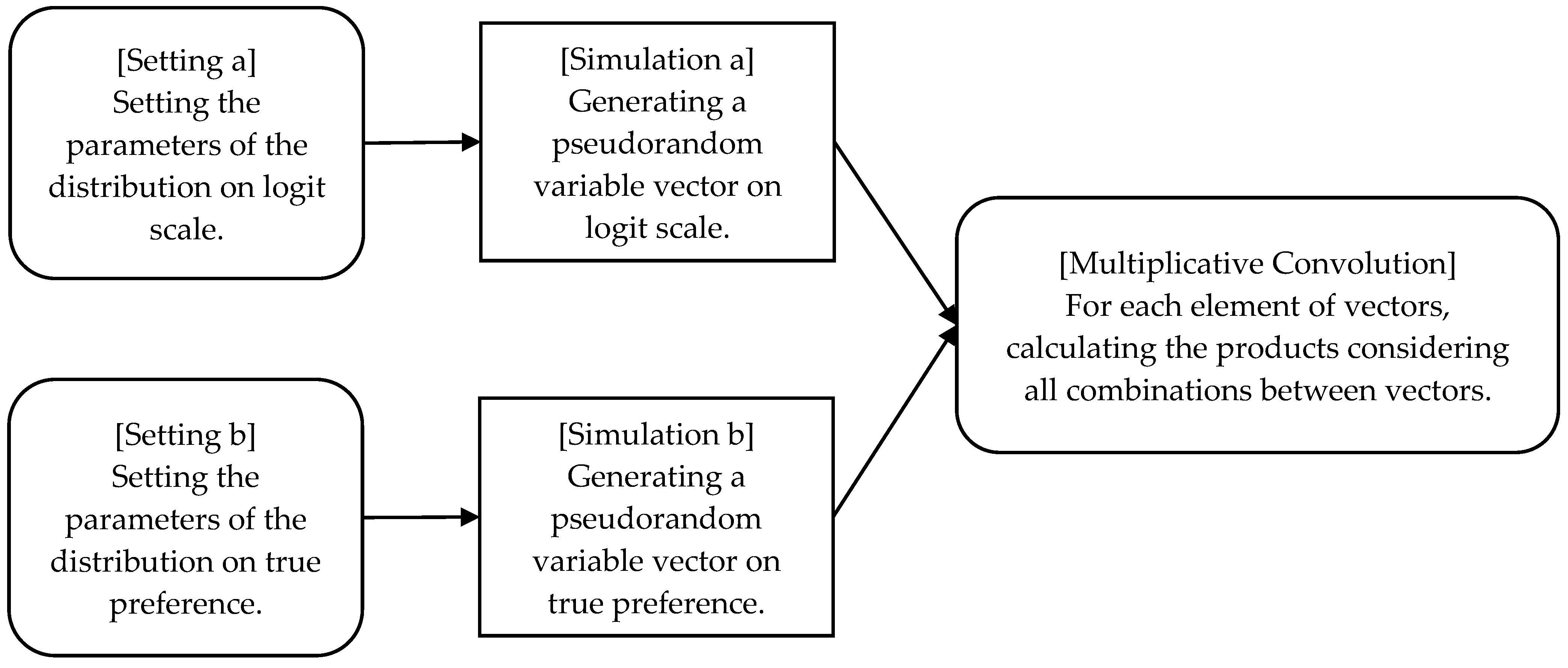
Appendix C. Simple Algorithm Diagram of the Simulations in This Paper

Figure A1. Simple Algorithm Diagram of the Simulations in this Paper.
Mathematics 11 04727 g0a1

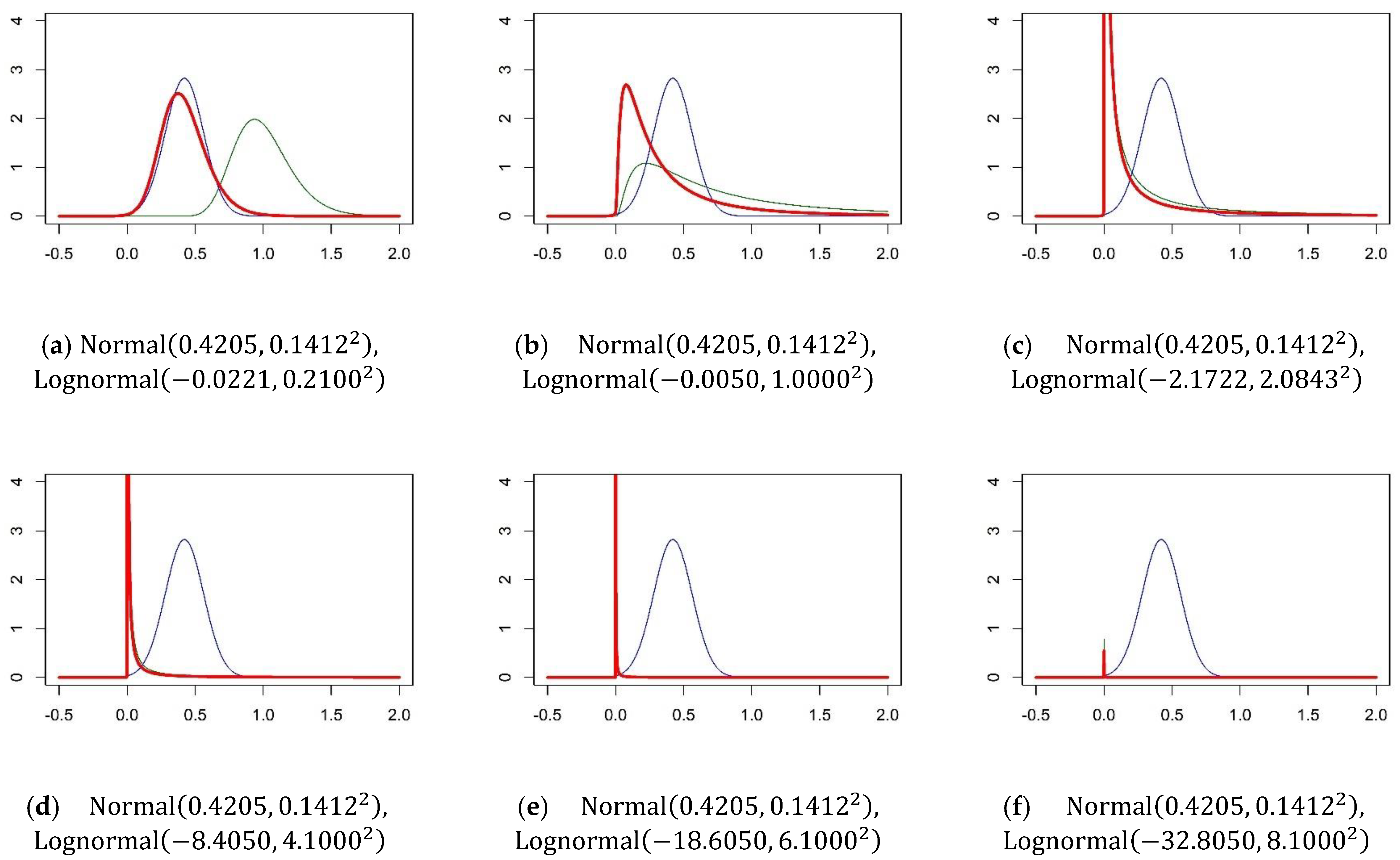
Appendix D. Properties of the Lognormal Distribution of the Logit Scale in the G-MNL Model

Now, r 1 ˜ N o r m a l a 1 , b 1 2 and r 2 ˜ N o r m a l a 2 , b 2 2 are statistically independent. Then, e x p r 1 ˜ L o g n o r m a l a 1 , b 1 2 , and e x p r 2 ˜ L o g n o r m a l a 2 , b 2 2 , respectively. The product of the two is e x p r 1 e x p r 2 = e x p r 1 + r 2 . From the reproducibility of the normal distribution, r 1 + r 2 ˜ N o r m a l a 1 + a 2 , b 1 2 + b 2 2 . Therefore, e x p r 1 + r 2 ˜ L o g n o r m a l a 1 + a 2 , b 1 2 + b 2 2 . Thus, when the logit scale and true preference parameters both follow a lognormal distribution in the G-MNL model, the product of the two, the apparent preference, also follows a lognormal distribution.
In the G-MNL model, φ ˜ L o g n o r m a l μ φ , τ , 0 < φ < , let r ˜ N o r m a l μ r , σ r 2 , < r < , and 0 < φ = e x p r < ; then:
lim τ 0 1 2 π τ φ e x p ln φ μ φ 2 2 τ 2 = 1 φ lim τ 0 1 2 π τ e x p r μ φ 2 2 τ 2
= δ r μ φ φ
= δ ln φ μ φ φ .
E φ = 1 , then, μ φ = τ 2 / 2 . The probability density function according to the apparent preference parameters can be obtained from Rohatgi and Saleh [36]. As τ 0 , μ φ 0 , and:
l i m τ 0 f β β = l i m τ 0 1 φ f φ φ f α β φ d φ
= l i m τ 0 1 φ δ ln φ μ φ φ f α β φ d φ
= l i m τ 0 δ ln φ μ φ 1 φ 2 f α β φ d φ
= l i m τ 0 δ φ e x p μ φ 1 φ 2 f α β φ d φ
= 1 1 2 f α β 1
= f α β .
Thus, it matches the probability distribution according to the true preference parameters. Additionally, when τ , from l’Hôpital’s rule, it follows that:
lim τ 1 2 π τ φ e x p ln φ μ φ 2 2 τ 2 = 1 φ lim τ 1 2 π τ e x p ln φ + τ 2 / 2 2 2 τ 2
= 1 φ 1 2 π l i m τ τ exp l i m τ 2 τ ln φ + τ 2 / 2 4 τ
= 1 φ 1 2 π l i m τ τ exp l i m τ ln φ + τ 2 / 2 2
= 1 2 π φ · 0 · 0 = 0 .

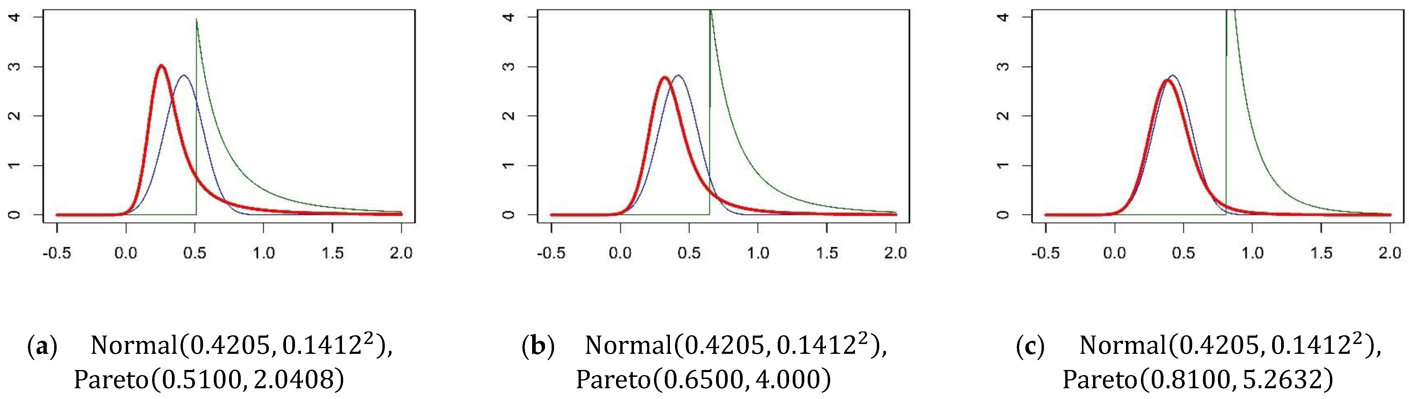
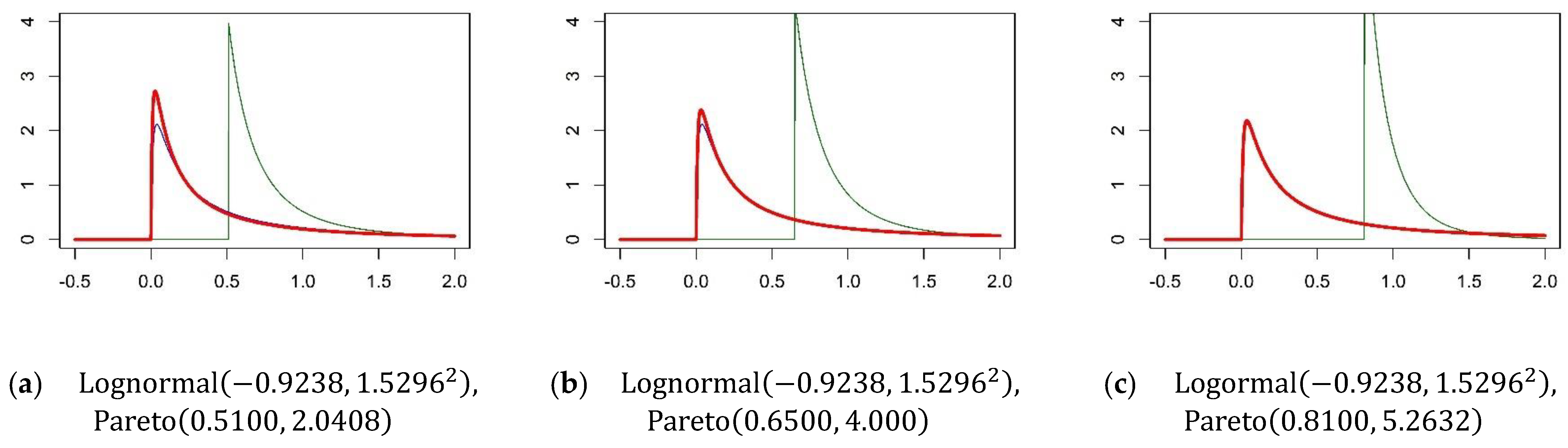
Appendix E. Properties of Type I Pareto Distribution of Logit Scale in the MIXL-iPS Model

Here, we consider the case where the logit scale follows the Pareto distribution type I, i.e., φ ˜ P a r e t o κ , ζ . Let us suppose κ < φ . As ζ , ζ κ , and φ / κ ζ + 1 . Then, from l’Hôpital’s rule, the probability density function is:
lim ζ , κ < φ f φ φ = lim ζ , κ < φ ζ κ lim ζ , κ < φ φ / κ ζ + 1 = lim ζ , κ < φ κ lim ζ , κ < φ ζ φ / κ ζ = 0 .
Additionally, let us suppose κ = φ . Then:
lim ζ , κ = φ f φ φ = lim ζ , κ = φ ζ κ = .
Therefore,
lim ζ f φ φ = δ φ κ .
Then, from the constraint of expected value 1, we can see that:
V a r φ = ζ κ 2 ζ 1 2 ζ 2
= ζ κ ζ 1 · κ ζ 1 ζ 2
= κ ζ 1 ζ 2
= κ 1 1 κ 1 1 1 κ 2
= κ 1 κ 2 1 1 + κ 1 2 + 2 κ
= κ 1 κ 2 κ 1 + 2 κ
= 1 κ 2 1 + 2 κ .
Let us consider the following, where ξ is the Gumbel scale of the Gumbel distribution G u m b e l 0 , ξ . When φ = 1 / ξ follows a Pareto distribution P a r e t o κ ,   ζ , ξ follows a power-function distribution. The probability density function and cumulative distribution function become [49]:
f ξ ξ = ζ κ ζ ξ ,   F ξ ξ = κ ξ ζ   0 ξ 1 κ ,   0 < ζ
Let us suppose E φ = 1 ; then, from the fact that 1 / 2 < κ < 1 , the MIXL-iPS model has a Gumbel scale of at most 0 ξ < 2 , and for the Gumbel error variance of ARUM before the redefinition, it assumes a reasonable range of possible values of at most 0 ξ 2 π 2 / 6 < 4 π 2 / 6 2.094 . We note that E ξ = 1 ; thus, the Gumbel scale here should be considered relatively.

References

  1. McFadden, D. Conditional logit analysis of qualitative choice behaviour. In Frontiers in Econometrics; Zarembka, P., Ed.; Academic Press: Berkwlly, CA, USA, 1974; pp. 105–142. [Google Scholar]
  2. Yellott, J.I. The relationship between Luce’s choice axiom, Thurstone’s theory of comparative judgment, and the double exponential distribution. J. Math. Psychol. 1977, 15, 109–144. [Google Scholar] [CrossRef]
  3. Luce, R.D. Individual Choice Behavior: A Theoretical Analysis; Wiley: New York, NY, USA, 1959. [Google Scholar]
  4. Thurstone, L.L. A law of comparative judgment. Psychol. Rev. 1927, 34, 273–286. [Google Scholar] [CrossRef]
  5. McKelvey, R.D.; Palfrey, T.R. Quantal response equilibria for normal form games. Games Econ. Behav. 1995, 10, 6–38. [Google Scholar] [CrossRef]
  6. Simon, H.A. Administrative Behavior: A Study of Decision-Making Processes in Administrative Organization; Macmillan Publishers: New York, NY, USA, 1947. [Google Scholar]
  7. Ratcliff, R. A theory of memory retrieval. Psychol. Rev. 1978, 85, 59–108. [Google Scholar] [CrossRef]
  8. Bogacz, R.; Brown, E.; Moehlis, J.; Holmes, P.; Cohen, J.D. The physics of optimal decision making: A formal analysis of models of performance in two-alternative forced-choice tasks. Psychol. Rev. 2006, 113, 700–765. [Google Scholar] [CrossRef]
  9. Webb, R. The (neural) dynamics of stochastic choice. Manag. Sci. 2019, 65, 230–255. [Google Scholar] [CrossRef]
  10. Davis-Stober, C.P.; Brown, N.; Park, S.; Regenwetter, M. Recasting a biologically motivated computational model within a Fechnerian and random utility framework. J. Math. Psychol. 2017, 77, 156–164. [Google Scholar] [CrossRef]
  11. Hensher, D.; Rose, J.; Greene, W. Applied Choice Analysis; Cambridge University Press: Cambridge, UK, 2015. [Google Scholar]
  12. Louviere, J.J.; Hensher, D.A.; Swait, J.D. Stated Choice Methods: Analysis and Applications; Cambridge University Press: Cambridge, UK, 2000. [Google Scholar]
  13. Train, K. Discrete Choice Methods with Simulation; Cambridge University Press: Cambridge, UK, 2009. [Google Scholar]
  14. Meißner, M.; Decker, R. Eye-tracking information processing in choice-based conjoint analysis. Int. J. Mark. Res. 2010, 52, 593–612. [Google Scholar] [CrossRef]
  15. Revelt, D.; Train, K. Mixed logit with repeated choices: Households’ choices of appliance efficiency level. Rev. Econ. Stat. 1998, 80, 647–657. [Google Scholar] [CrossRef]
  16. Hausman, J.A.; Wise, D.A. A conditional probit model for qualitative choice: Discrete decisions recognizing interdependence and heterogeneous preferences. Econometrica 1978, 46, 403–426. [Google Scholar] [CrossRef]
  17. McFadden, D.; Train, K. Mixed MNL models for discrete response. J. Appl. Econom. 2000, 15, 447–470. [Google Scholar] [CrossRef]
  18. Hess, S.; Train, K. Correlation and scale in mixed logit models. J. Choice Model. 2017, 23, 1–8. [Google Scholar] [CrossRef]
  19. Fiebig, D.G.; Keane, M.P.; Louviere, J.; Wasi, N. The generalized multinomial logit model: Accounting for scale and coefficient heterogeneity. Mark. Sci. 2010, 29, 393–421. [Google Scholar] [CrossRef]
  20. Greene, W.H.; Hensher, D.A. Does scale heterogeneity across individuals matter? An empirical assessment of alternative logit models. Transportation 2010, 37, 413–428. [Google Scholar] [CrossRef]
  21. Ohdoko, T. Preliminary examination of generalized multinomial logit subclasses on choice experiments: Japanese undergraduate survey data on a takeaway cup of fair trade coffee. J. Inform. 2015, 6, 14–36, (with Japanese title and abstract). [Google Scholar]
  22. Adamska, J.; Bielak, Ł.; Janczura, J.; Wyłomańska, A. From multi-to univariate: A product random variable with an application to electricity market transactions: Pareto and student’s t-distribution Case. Mathematics 2022, 10, 3371. [Google Scholar] [CrossRef]
  23. Arnold, B.C. Pareto Distributions; Routledge: New York, NY, USA, 2015. [Google Scholar]
  24. Rezapour, M.; Ksaibati, K. Accommodating taste and scale heterogeneity for front-seat passenger’ choice of seat belt usage. Mathematics 2021, 9, 460. [Google Scholar] [CrossRef]
  25. Marsili, M. On the multinomial logit model. Phys. A Stat. Mech. Appl. 1999, 269, 9–15. [Google Scholar] [CrossRef]
  26. Cover, T.M.; Thomas, J.A. Elements of Information Theory; John Wiley & Sons, Inc.: Hoboken, NJ, USA, 2006. [Google Scholar]
  27. Wang, H.; Yan, X.Y.; Wu, J. Free utility model for explaining the social gravity law. J. Stat. Mech. Theory Exp. 2021, 2021, 033418. [Google Scholar] [CrossRef]
  28. Brown, T.C.; Kingsley, D.; Peterson, G.L.; Flores, N.E.; Clarke, A.; Birjulin, A. Reliability of individual valuations of public and private goods: Choice consistency, response time, and preference refinement. J. Public Econ. 2008, 92, 1595–1606. [Google Scholar] [CrossRef]
  29. Swait, J.; Louviere, J. The role of the scale parameter in the estimation and comparison of multinomial logit models. J. Mark. Res. 1993, 30, 305–314. [Google Scholar] [CrossRef]
  30. Uggeldahl, K.; Jacobsen, C.; Lundhede, T.H.; Olsen, S.B. Choice certainty in discrete choice experiments: Will eye tracking provide useful measures? J. Choice Model. 2016, 20, 35–48. [Google Scholar] [CrossRef]
  31. Hess, S.; Stathopoulos, A. Linking response quality to survey engagement: A combined random scale and latent variable approach. J. Choice Model. 2013, 7, 1–12. [Google Scholar] [CrossRef]
  32. Daly, A.; Hess, S.; Train, K. Assuring finite moments for willingness to pay in random coefficient models. Transportation 2012, 39, 19–31. [Google Scholar] [CrossRef]
  33. Hess, S.; Palma, D. Apollo: A flexible, powerful and customisable freeware package for choice model estimation and application. J. Choice Model. 2019, 32, 100170. [Google Scholar] [CrossRef]
  34. Mariel, P.; Artabe, A. Interpreting correlated random parameters in choice experiments. J. Environ. Econ. Manag. 2020, 103, 102363. [Google Scholar] [CrossRef]
  35. Grüne-Yanoff, T. What preferences for behavioral welfare economics? J. Econ. Methodol. 2022, 29, 153–165. [Google Scholar] [CrossRef]
  36. Rohatgi, V.K.; Saleh, A.M.E. An Introduction to Probability and Statistics; John Wiley & Sons: Hoboken, NJ, USA, 2015. [Google Scholar]
  37. R Core Team. R: A Language and Environment for Statistical Computing; R Foundation for Statistical Computing: Vienna, Austria, 2022. [Google Scholar]
  38. Hess, S.; Rose, J.M. Can scale and coefficient heterogeneity be separated in random coefficients models? Transportation 2012, 39, 1225–1239. [Google Scholar] [CrossRef]
  39. Ruckdeschel, P.; Kohl, M. General purpose convolution algorithm in S4 classes by means of FFT. J. Stat. Softw. 2014, 59, 1–25. [Google Scholar] [CrossRef]
  40. Ankamah-Yeboah, I.; Asche, F.; Bronnmann, J.; Nielsen, M.; Nielsen, R. Consumer preference heterogeneity and preference segmentation: The case of ecolabeled salmon in Danish retail sales. Mar. Resour. Econ. 2020, 35, 159–176. [Google Scholar] [CrossRef]
  41. Haaijer, R.; Wedel, M.; Vriens, M.; Wansbeek, T. Utility covariances and context effects in conjoint MNP models. Mark. Sci. 1998, 17, 236–252. [Google Scholar] [CrossRef]
  42. DeShazo, J.R.; Fermo, G. Designing choice sets for stated preference methods: The effects of complexity on choice consistency. J. Environ. Econ. Manag. 2002, 44, 123–143. [Google Scholar] [CrossRef]
  43. Matějka, F.; McKay, A. Rational inattention to discrete choices: A new foundation for the multinomial logit model. Am. Econ. Rev. 2015, 105, 272–298. [Google Scholar] [CrossRef]
  44. Fosgerau, M.; Melo, E.; de Palma, A.; Shum, M. Discrete choice and rational inattention: A general equivalence result. Int. Econ. Rev. 2020, 61, 1569–1589. [Google Scholar] [CrossRef]
  45. Friston, K.; Rigoli, F.; Ognibene, D.; Mathys, C.; Fitzgerald, T.; Pezzulo, G. Active inference and epistemic value. Cogn. Neurosci. 2015, 6, 187–214. [Google Scholar] [CrossRef]
  46. Grebitus, C.; Jutta, R.; Carolin, C.S. Visual attention and choice: A behavioral economics perspective on food decisions. J. Agric. Food Ind. Organ. 2015, 13, 73–81. [Google Scholar] [CrossRef]
  47. Bishop, C.M.; Nasrabadi, N.M. Pattern Recognition and Machine Learning; Springer: New York, NY, USA, 2006. [Google Scholar]
  48. Hinton, G.; Vinyals, O.; Dean, J. Distilling the knowledge in a neural network. arXiv 2015, arXiv:1503.02531. [Google Scholar] [CrossRef]
  49. Dallas, A.C. Characterizing the pareto and power distributions. Ann. Inst. Stat. Math. 1976, 28, 491–497. [Google Scholar] [CrossRef]
Figure 1. Multiplicative convolution of normal and lognormal distributions in the G-MNL model type II. Note: The blue line is the normal distribution; the green line is the lognormal distribution with expectation 1; and the red line is the multiplicative convolution of the two distributions. The absolute values of the estimated mean and standard deviation parameters of the travel cost per Hess and Rose [38] were used for the normal distribution. We looked at the effect of the standard deviation of the lognormal distribution of the logit scale around the estimate of Hess and Rose [38]. Panel (c) represents the result by using the variance estimate on the logit scale used in Hess and Rose [38].
Mathematics 11 04727 g001
Figure 2. Multiplicative convolution of the MIXL-iPS model’s normal distribution and Pareto distribution type I. Note: The blue line is the normal distribution; the green line is the Pareto distribution type I with expectation 1; the red line is the multiplicative convolution of the two distributions; the absolute values of the estimated mean and standard deviation parameters of the travel cost as taken from Hess and Rose [38] were used for the normal distribution.
Mathematics 11 04727 g002
Figure 3. Multiplicative convolution of the lognormal and Pareto distribution type I of the MIXL-iPS model. Note: The blue line is the lognormal distribution; the green line is the Pareto distribution type I with expectation 1; the red line is the multiplicative convolution of the two distributions. Estimates of the mean and standard deviation parameters of travel cost as taken from Hess and Rose [38] were used for the lognormal distribution.
Mathematics 11 04727 g003
Disclaimer/Publisher’s Note: The statements, opinions and data contained in all publications are solely those of the individual author(s) and contributor(s) and not of MDPI and/or the editor(s). MDPI and/or the editor(s) disclaim responsibility for any injury to people or property resulting from any ideas, methods, instructions or products referred to in the content.

