Article

A Data-Driven Convolutional Neural Network Approach for Power Quality Disturbance Signal Classification (DeepPQDS-FKTNet)

by
Fahman Saeed
1,*,
Sultan Aldera
1,
Mohammad Alkhatib
1,
Abdullrahman A. Al-Shamma’a
2 and
Hassan M. Hussein Farh
2
1
Computer Science Department, College of Computer and Information Sciences, Imam Mohammad Ibn Saud Islamic University (IMSIU), Riyadh 11432, Saudi Arabia
2
Electrical Engineering Department, College of Engineering, Imam Mohammad Ibn Saud Islamic University (IMSIU), Riyadh 11432, Saudi Arabia
*
Author to whom correspondence should be addressed.
Mathematics 2023, 11(23), 4726; https://doi.org/10.3390/math11234726
Submission received: 5 November 2023 / Revised: 17 November 2023 / Accepted: 20 November 2023 / Published: 22 November 2023
(This article belongs to the Special Issue AI Algorithm Design and Application)

Abstract

:
Power quality disturbance (PQD) signal classification is crucial for the real-time monitoring of modern power grids, assuring safe and reliable operation and user safety. Traditional power quality disturbance signal classification approaches are sensitive to noise, feature selection, etc. This study introduces a novel approach utilizing a data-driven convolutional neural network (CNN) to improve the effectiveness of power quality disturbance signal classification. Deep learning has been successfully used in various fields of recognition, yielding promising outcomes. Deep learning is often characterized as a complex system, with its filters and layers being determined through empirical investigations. A deep learning model was developed for the purpose of classifying PQDs, with the aim of narrowing down the search for unidentified PQDs to a specific problem domain. This approach demonstrates a high level of efficiency in accelerating the process of recognizing PQDs among a vast database of PQDs. In order to automatically identify the number of filters and the number of layers in the model in a PQD dataset, the proposed model uses pyramidal clustering, the Fukunaga–Koontz transform, and the ratio of the between-class scatter to the within-class scatter. The suggested model was assessed using the synthetic dataset generated, with and without the presence of noise. The proposed models outperformed both well-known pre-trained models and state-of-the-art PQD classification techniques in terms of classification accuracy.

1. Introduction

Power quality (PQ) means the state of the energy being consumed. The term “Power Quality” (PQ) refers to the properties of electricity at a specific location in an electrical system compared with a standard set of values. Power quality disturbances (PQDs) are, thus, detectable by electrical power providers and consumers as variations in these characteristics from the reference parameters. As a result, PQDs are measured and graded in terms of both voltage and current quality. These disruptions may be caused by a number of factors: Power outages can occur as a result of natural causes such as lightning strikes, severe weather, or earthquakes [1]. Disturbances to power quality can also be caused by human activity, such as when machinery fails, switches are activated, or the grid is overloaded [2]. Power quality issues might arise due to the progressive degradation of power equipment as it ages. One common form of power interruption is sags, which are characterized by voltage decreases. These occurrences can be attributed to several factors such as lightning strikes and mechanical failures. Voltage surges, also known as voltage swells, are seen. These swells are further influenced by the actions of switching and the grid’s overload. A complete cessation of electrical power can occur as a result of three distinct disruptions, which can be attributed to either natural calamities or the malfunctioning of machinery. The illumination inside the designated area experiences an abrupt and intermittent fluctuation. Flicker is a phenomenon that arises due to the presence of sagging, swelling, and harmonics. The harmonics of a power signal consist of multiples of the fundamental frequency. Harmonics can arise as a consequence of electronic equipment and various other causes [3].
It is possible for electronic equipment to be damaged by fluctuations in the power supply. Disruptions in power quality can erase information stored on computers and other electronic devices. Problems with the power supply could result in brownouts or complete blackouts, disrupting service. There are a variety of countermeasures available. Your electronics can be safeguarded by using surge protectors, filters, and an uninterruptible power supply (UPS) [4]. According to data gathered in the USA, it is estimated that customers are responsible for approximately 70% of PQ interruptions, while network operators are to blame for the other 30% [5]. Every country has its own unique PQ challenges. In both European and American countries, harmonics accounts for less than a fifth of all PQ issues, while it accounts for approximately a quarter of all PQ issues in the United States [5]. As a result, not every PQ problem can be solved with a single formula. There must be a more detailed and precise estimate of the price. Therefore, PQ monitoring systems for detecting and classifying PQDs are crucial in the smart grid paradigm. The time and location of voltage and current fluctuations can be gleaned from the detection phase, while the classification phase aids in the identification of disturbances and their causes [6].
Several approaches to the problems of PQD detection and classification in online and real-time systems have been developed. Handcraft methods for feature extraction review are presented in [7,8]; different artificial intelligence (AI) methods for categorizing PQ events are discussed in [9]; and deep learning algorithms and transformers can detect and categorize power quality issues. High-accuracy classification has been achieved with the use of deep recurrent neural network (DRNN) classifiers such as bidirectional long short-term memory (BiLSTM) architectures [10]. Robust feature extraction from power measurement data can also be achieved with the use of transformers, such as the univariate temporal convolutional denoising autoencoder (UTCN-DAE) [11]. Fault prediction in power distribution networks has also made use of machine learning approaches, such as linear and non-linear classifiers [12]. Power quality disturbance identification has also been improved with a hybrid detection method that combines wavelet transform and a convolutional neural network (CNN) [13]. S-transform- and LeNet-5-based power quality disturbance categorization is proposed in [14]. The suggested algorithm can accurately categorize single disturbance signals with varying signal-to-noise ratios and composite disturbance signals made of single disturbance signals. It also has strong noise immunity. The LeNet-5 input form distinguishes this method from others. The disturbance signal’s gray picture is input via traditional means.
The suggested technique in [15] is compared with many current methods for the classification of PQDs from two types of data sources. Datasets from the IEEE Work Group P1159.3 and P1159.2 comprise seven types of individual power quality disturbances and eleven types of combined disturbances, and the findings show that the new method can more accurately classify both single and combined PQDs. In the research in [16], an adaptive neuro-fuzzy algorithm based on the discrete packet wavelet transform and the Kalman filter is proposed for detecting and categorizing power quality events in distributed generation systems (DGs). The suggested method outperforms state-of-the-art classification techniques in terms of classification accuracy, convergence time, and error prediction. This technique outperformed both a fuzzy logic adaptive system based on the discrete wavelet transform and an artificial neural network based on the Fourier transform when constructed and evaluated in MATLAB. They used artificially produced power quality indications using MATLAB, including voltage sag, voltage swell, flicker, and harmonics, to assess the effectiveness of their system and obtained an accuracy of 98%. Figure 1 delineates an expansive flowchart categorizing power quality issues into distinct classifications, encompassing transients, long- and short-duration voltage variations, voltage imbalance, waveform distortions, flicker, and their repercussions on end-user devices. Each category includes specific issues such as sags, swells, harmonics, and noise, which are further explained.
As they now stand, deep learning models are a mystery. There is no hard and fast rule for selecting which layers and filters to utilize; rather, they are determined experimentally. We applied these data in a novel approach to develop an adaptable deep learning model motivated by the PQD dataset. we derived the layer filters using the Fukunaga–Koontz transform (FKT) [18]. To control the depth of the CNN model, we computed the ratio between the trace between scatter matrix Sb and within scatter matrix Sw. The DeepFKTNet model [19] was developed for fingerprint classification. DeepFKTNet extracts LGDBP [20] features from fingerprints and then clusters them using the K-medoids [21] clustering algorithm. It uses the eigenvectors as filters for the CNN layers. Its architecture works with 2D fingerprints, whereas our PQD data are 1D.
The proposed PQD CNN classification system was evaluated against the state-of-the-art PQD classification schemes utilizing the synthetic dataset generated based on IEEE Std-1159-2009. Our technique makes the following significant contributions:
  • An intelligent computer method for classifying PQDs has been developed.
  • A constructive method is proposed for automatically constructing a data-driven CNN model with a custom-designed architecture by utilizing clustering, FKT, and the ratio of the traces of the between-class scatter matrix and the within-class scatter matrix to extract discriminative information from the 1D PQD dataset.
  • The obtained results reveal that the proposed PQDs classification scheme is quick, accurate, and performs well.
This paper is organized as follows: Section 1 contains the introduction, Section 2 contains the proposed method, Section 3 contains the experimental results, and Section 4 contains the conclusion.

2. Proposed Method

2.1. Adaptive CNN Model

The search for the optimal model configuration for a given application is a challenging optimization issue because of the large parameter space that must be explored. A convolutional (CONV) layer is the backbone of any convolutional neural network (CNN) model. The CONV layer uses a predetermined number of filters to perform convolution operations on the input signal, thereby extracting discriminative features. For a CNN model to derive a feature hierarchy, the CONV layers must be layered. Among the most difficult hyperparameters to tune for a given application are the number of CONV layers and the number of filters in each layer. Model performance is highly sensitive to the initialization of learnable parameters when using iterative optimization approaches like the Adam optimizer. Adaptive model design can be determined with relative ease by utilizing the discriminative content of PQDs. To begin, we cluster each type of PQD in the dataset to find suitable examples from which to construct a CNN model. Each CONV layer’s breadth (number of filters) and depth (number of CONV layers) are set with the information that identifies the main trends and patterns and differentiates chosen PQDs. The overall design procedure is depicted in Figure 2.
We offer a straightforward approach to adaptively determining the optimal model configuration by exploiting the discriminative content of PQDs. To begin, we choose exemplary PQDs to serve as our pointers while we develop our CNN model. Data-dependent initialization of CONV layer filters is performed using the discriminative information in these PQDs to establish the model’s width (the number of filters in each CONV layer) and depth (the number of CONV layers). An overview of the design process is shown in Figure 2. To select the representative PQDs, we use clustering. To select the number of filters in a CONV layer, we use the Fukunaga–Koontz transform (FKT) [18], which makes use of class-discriminative information, and we use the ratio of the between-class scatter matrix Sb to the within-class scatter matrix Sw to select the suitable depth (i.e., the number of CONV layers) of the CNN model. In order to reduce the amount of trainable parameters and prevent overfitting, global pooling layers are implemented. This fits very well with the CONV architecture since it ensures uniformity in feature maps and classes [22] and feeds its results straight into SoftMax layers. In the sections that follow, we will discuss the specifics of the design process, and Figure 2 provides a high-level view.

2.1.1. Selection of Representative PQDs

In order to adaptively specify the CONV layers and the depth of the CNN model, we choose the representative PQDs. In step 2 of Algorithm 1, we carry this out by identifying the most representative PQDs of each class by clustering the training set. K-medoids [21] is used for clustering to determine the representative PQDs since it is appropriate for finding the representative subset of the training set, and it picks the instances as cluster centers. The PQDs that are located in the centers of the clusters are selected for this purpose. Using silhouette analysis [23], the K-medoids algorithm’s number of clusters for each class is given.
Algorithm 1: Design of the main DeepPQDS-FKTNet architecture
Input: The set PS = (PS1, PS2, …, PSC), where c is the number of classes and PSi = (PQDj, j = 1, 2, 3, , ni) is the set of PQD signals of the ith class.
Output: The main DeepPQDS-FKTNet architecture.
Step 1:
Initialize DeepPQDS-FKTNet with the input layer and set w = 3, h = 1, d = 1, and m (the number of filters) = 0 for the first layer and PTR (previous TR) = 0.
Step 2:
For i = 1, 2, 3, …, C: c is the number of classes.
  • Compute Z i = ( a j i = R P Q D j ) where R P Q D j is the representative PQDs (centers of clusters) extracted using the K-medoid clustering algorithm from PS.
Step 3:
For i = 1, 2, 3,…, C
  Ai = ∅
  For each a j i Z i
  • Divide the PQD signal into patches of size w × 1 with stride 1: P 1 i , P 2 i , ,   P m i i from a j i .
  • Apply K-medoid clustering and return the representative patches R P i = ( P 1 i , P 2 i , ,   P c e i i ) , s u c h   t h a t   c e i   i s   t h e   n u m b e r   o f   c l u s t e r   c e n t e r s   o f   t h e   i t h   r e p r e s e n t a t i v e
  • Combine the representative patches R P i
                        P = ( P 1 1 , P 2 2 , , P m n n ) , s u c h   t h a t   P 1 I     R l : l   i s   t h e   l e n g t h   o f   P Q D and append to Ai.
Step 4:
Using A = [A1, A2, …, AC], compute
  • Between-class scatter matrix S b = i = 1 C ( 1 n i A i J i 1 n A J ) ( 1 n i A i J i 1 n A J ) T , where J i is an n i × n i matrix with all ones.
  • Within-class scatter matrices S w = i = 1 C ( A i 1 n i A i J i ) ( A i 1 n i A i J i ) T .
Step 5:
Diagonalize the sum ∑ = Sb + Sw i.e., = Q D Q T and transform the scatter matrices using the transform matrix P = Q D 1 2 , i.e.,   S b ^ = P T S b P , S w ^ = P T S w P .
Step 6:
Compute eigenvectors u k , k = 1,2 , , D of S b ^ such that S b ^ u = λ u .
Step 7:
For each eigenvector u k , k = 1,2 , , D
  • Compute Y = Y 1 , Y 2 , , Y C , where Y i = ( u k a j i , j = 1,2 , , n i ) .
  • Compute the between scatter matrix SPQDb and within scatter matrix SPQDw from Y .
  • Compute the trace ratio γ k = T r a c e ( S P Q D b ) T r a c e ( S P Q D w ) .
Step 8:
Select L filters u l , k = 1,2 , , L corresponding to γ k > 0 (as shown in Figure 3 for layer 1).
Step 9:
Add the CONV block to DeepPQDS-FKTNet with filters u l , k = 1,2 , , L . Update m = m + 1.
Step 10:
If m = 1 or 2, add a max pool layer with a pooling operation of size 2 × 1 and stride 2 to DeepPQDS-FKTNet.
Step 11:
Compute Z = ( Z 1 ,   Z 2 ,   ,   Z C ) , where Z i = ( a j i = DeepPQDS-FKTNet(RPQDj), for each R P Q D j P Q D i )
Step 12:
Using Z = ( Z 1 ,   Z 2 ,   ,   Z C ) ,
  • Compute the ratio T R = T r a c e ( S b ) T r a c e ( S w ) ,   where S b and S w are the between-class and within-class scatter matrices of the activations Z .
  • If P T R   T R ,     s e t   P T R = T R , d = L, and go to Step 3; otherwise, stop.
Figure 3. Selection of best filters for layer 1 of DeepPQDS-FKTNet model for synthetic PQD dataset.
Mathematics 11 04726 g003

2.1.2. Design of the Main DeepPQDS-FKTNet Architecture

State-of-the-art CNN models typically have set, extremely intricate topologies that are not derived from the data. Instead, we establish a data-dependent framework for DeepPQDS-FKTNet. Its fundamental structure is determined by how many CONV layers the model needs and how many filters should be used in each of those layers. An iterative technique is developed to answer these questions. It calculates the number of filters in a CONV layer, adds that layer iteratively to the model, and stops when some condition is met. The number of filters in a CONV layer and how they are initially set are both determined by the discriminative information included in PQDs. Algorithm 1 provides the specifics. In the next paragraphs, we provide an explanation of the algorithm and its rationale.
Initially, the set of PQD: PS = (PS1, PS2, , PSC), is used to determine the number of filters in the first CONV layer and initialize them. Unlike the filter size of the first CONV layer in state-of-the-art CNN models like ResNet [24], DenseNet [25], and Inception [26], we fixed the filter size of the first layer to 3 × 1. Using a filter of size 3 is usually best for 1D PQD data. This captures less input data but produces less output data. This simplifies model training. After extracting the representative PQDs in step 2, we specify the discriminated patches of the current layer by choosing the patches P 1 i , P 2 i , ,   P m i i of size 3 × 1 from each PQD and then cluster them using the procedure in step 3 and select the patches in the clusters’ centers to form the covariance matrix in the fourth step of the method. The 1D representative patches from each PQD, where P = ( P 1 1 , P 2 2 , ,   P m n n ) , s u c h   t h a t   P 1 I     R d , are combined in such a way that FKT makes use of the distinct features of the patches in the set P to eliminate overlapping elements and count the number of occurrences of each filter type. In stages 2–3 of the Algorithm 1, we pick patches from the representative PQDs with a size of w × 1, and recast the problem of selecting the filters (uk, k = 1, 2, … N) as finding the optimal projection direction vectors, ul, l = 1, 2, … d, by addressing the optimization problem below:
U * = a r g max U t r ( U T S b U ) t r ( U T S w U ) ,  
where the scatter matrices across classes (Sb) and within classes (Sw) (as computed in step 7 of the Algorithm 1) are revealed with a discriminant function of Fukunaga and Koontz (FKT) [18]. The optimal projection direction vectors u i are the eigenvectors of S b ^ , i.e.,
S b ^ u = λ u  
where S b ^ = P T S b P , P = Q D 1 / 2 , and Q and D are computed by diagonalizing the total S b + S w , i.e., S b + S w = Q D Q T (steps 5–6 of the Algorithm 1). Suitable and optimal vectors are given using Equation (2) to maximize t r ( U T S b U ) and minimize t r U T S w U . This method can handle very high-dimensional data since, unlike LDA, the inversion of Sw is not required. Furthermore, the orthogonal best-possible vectors are sought after using this method. This method is appropriate for our architecture since the representative patch vectors, R P i , associated with the intermediate CONV layers have a high dimension, and we need filters that are decoupled and capture discriminating, not repeated, features.
The problem of selecting the number of filters in the convolutional layer is to select the eigenvectors u k ,   k = 1, 2, … K so that the ratio γ k = T r a c e ( S P Q D b ) T r a c e ( S P Q D w ) attains the maximum value. Herein, the between-class scatter matrix SPQDb and within-class matrix SPQDw are computed for each u k by projecting all activations a j i in the space spanned by u k (steps 7–8 of the Algorithm 1). This ensures the selection of the filters that extract discriminative features (15 filters, as shown in Figure 3). After selecting u l ,   k = 1, 2, … L, the CONV block with L filters u l , l = 1 , 2 , , L initialized with u l is introduced into DeepPQDS-FKTNet. Then, a pooling layer is added if needed (steps 9–10 of the Algorithm 1).
Using the current architecture of DeepPQDS-FKTNet, the set of activations Z = ( Z 1 ,   Z 2 ,   ,   Z C ) of PS = (PS1, PS2, …, PSC) is computed. These activations are used to determine whether to add more layers to the net. This is decided by calculating the trace ratio T R = T r a c e ( S b ) T r a c e ( S w ) , where S b and S w are the between-class and within-class scatter matrices of the activations Z . If the current TR is higher than the pre-current TR (PTR), then the current block of layers contributed to the network’s discriminative structure. This metric guarantees that DeepPQDS-FKTNet’s output features exhibit low intra-class dispersion and high inter-class variation. To add another CONV block, steps 3–8 are repeated with Z. To improve computational efficiency, pooling layers are placed after the first and second CONV blocks to lower the size of feature maps. Each layer can have a different set of filters due to the PQDs being used to determine the number of kernels.
It is important to keep in mind that the eigenvector u l used to determine the kernels of a CONV layer has the maximum   γ k and captures most of the variability in input PQD signals without redundancy in the form of independent features.
The complexity of a CNN model is heavily dependent on its depth (the number of layers) and the number of kernels (the number of kernels for each layer). Steps 7–8 of Algorithm 1 determine the best kernels that ensure the preservation of maximum energy of the input data and initialize these kernels to be suitable to the PQD domain. The selected kernels extract the features from PQDs so that the variability in the structures in the PQD domain is maximally preserved. As we delve deeper into the network, it becomes increasingly critical that the features be discriminative, i.e., have high inter-class variance and low intra-class scatter. This is ensured using the trace ratio T R = T r a c e ( S b ) T r a c e ( S w ) in step 12, where the larger the value of the trace ratio, the larger the inter-class variance and the smaller the intra-class scatter [27]. Step 12 in Algorithm 1 allows us to add CONV layers as long as TR is increasing and determines the data-dependent depth of DeepPQDS-FKTNet.

2.2. Problem Formulation

As shown in Table 1, the PQDs are categorized into nine distinct PQDs: normal, sag, swell, interruption, flicker, sag with harmonics, swell with harmonics, interruption with harmonics, and flicker with harmonics. Identifying the type of a PQD is considered a multiclass classification problem. Let there be K PQDs generated. These PQDs are categorized into C classes. Let P Q = ( P Q i j | 1   i K ,   ) , where P Q i j represents the ith PQD of the jth class c and c = (1, 2, …, C), where C is the number of distinct PQDs classes. predicting the type of Power Quality Disturbance (PQD), denoted as P Q i j to develop a function ψ that maps from the PQD space to a set of categories C. This involves taking a specific PQD, P Q i j , from the set PQ and assigning it a category label c from C, expressed as ( P Q i j   ,   θ) = c. In this expression, θ represents the parameters of the function. Herein, we use a convolutional neural network (CNN) model to craft the function ψ (which, in this case, represents the model’s weights and biases, and the model is constructed adaptively). Figure 2 depicts the design process, and the rest of this section provides further information.
The activation of the final convolutional block is represented by a tensor with dimensions h × 1 × L. This tensor is then passed as input to fully connected (FC) layers. However, due to the large number of parameters involved in these FC layers, there is a risk of overfitting. In order to decrease the number of parameters and spatial dimensions in the final convolutional block activation, it is common practice to input it into global average pooling (GAP) and global max-pooling (GMP) layers [29]. The GAP method calculates the average of all the h values, while the GMP method considers the contributions of the neurons with the largest response. In the fully connected (FC) layer, the number of neurons is h × 1 × L, but it is decreased to 1 × 1 × L when either GMP or GAP is used exclusively. The output of the GMP and GAP layers are concatenated in order to address the limitations of each layer. This concatenated output is then passed to the fully connected (FC) layer, which is subsequently followed by a SoftMax layer.

2.3. Fine Tuning the Model

The absence of a common database that may serve as a benchmark is currently a major barrier to the direct comparison of PQD classification systems [28]. There are various datasets that only display sag events or are datasets that only contain transient events. As stated in the listed related work, the available datasets are non-standard and vary in terms of the types of disturbances, sample sizes, [1 − α(u(t − t1) − u(t − t2))] labels applied to the data, and access techniques. Therefore, we tested our algorithm using open-source software that can generate synthetic power quality disruptions and was created just for comparing PQD classification techniques. The default duration of the generated signals was ten cycles, and the sampling rate for all signals was 3.2 kHz. The nominal frequency was adjusted to 50 Hz. The graphical user interface (GUI) was built using MATLAB 2016b, which was also used to generate the underlying code [28]. The 9 different forms of PQDs (normal, sag, swell, interruption, flicker, sag with harmonics, swell with harmonics, interruption with harmonics, and flicker with harmonics) were generated as presented in Table 1.
The synthetic dataset generator created two datasets. The first dataset had no noise, while the second featured random additive noise. White Gaussian noise has a 20–50 dB signal-to-noise ratio. The dataset comprises 18,000 signals with and without noise, each subset having 1000, wherein 90% of the dataset is used for training, while 10% is used for testing.
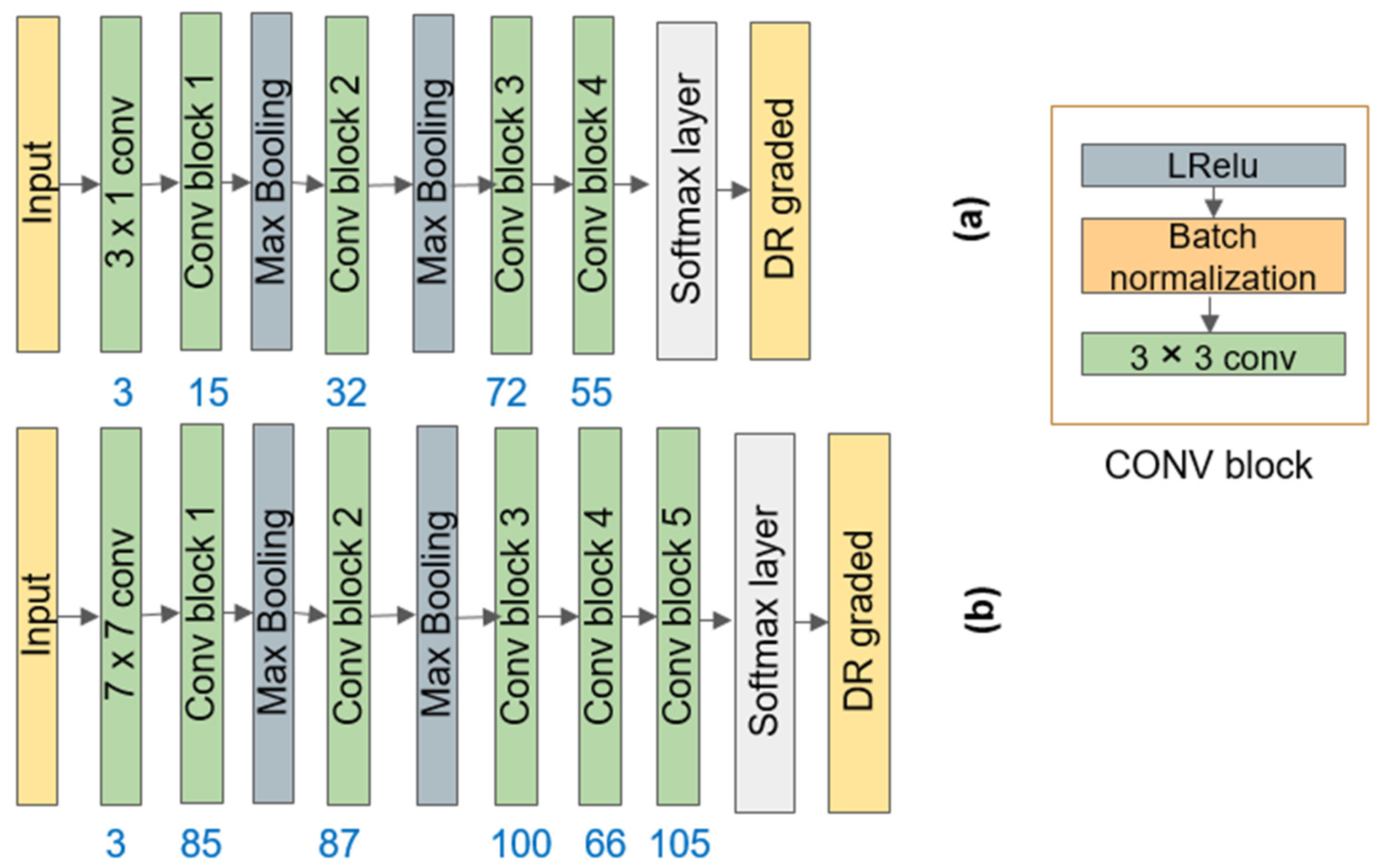
The performance of the DeepPQDS-FKTNet model was assessed by employing the synthetic dataset challenge, both with and without the presence of noise. The most representative PQD data from the training set were selected using the K-medoids algorithm. Subsequently, the adaptive DeepPQDS-FKTNet architecture was constructed using Algorithm 1. In order to establish the optimal parameters for the DeepPQDS-FKTNet model, the utilization of the hyperparameter optimization software framework Optuna was employed [30]. The DeepPQDS-FKTNet architecture obtained via the application of Algorithm 1 comprised 5 convolutional blocks without noise (Figure 4a) with number of filters (3, 15, 32, 72, and 55 filters for layers 1, 2,3, 4, and 5 consecutively) for the synthetic dataset. For the noisy dataset, the architecture consisted of 6 convolutional blocks with the maximum number of filters in each layer (3, 85, 87, 100, 66, and 105 filters for layers 1, 2,3, 4,5, and 6 consecutively), as the presence of noise introduces more complex patterns into the data (Figure 4b). The determination of the number of filters for each convolutional block and the depth of the model for the synthetic PQD dataset was accomplished via the utilization of Algorithm 1. The Optuna optimization algorithm was employed to fine-tune the hyperparameters in our study. Four different optimizers, namely, SGD, Adam, Adagrad, and RMSprop, were evaluated. The learning rate was varied within the range of 1 × 10⁻⁵ to 1 × 10⁻¹. Additionally, the patch size was explored using values of 8, 16, 24, and 48. Different activation functions, including Relu6, Sigmoid, Relu, and LRelu were also considered. Finally, the dropout rate was adjusted between 0.25 and 0.75. Following the completion of a training process spanning 10 epochs, the optimal hyperparameters for the dataset were documented and are presented in Table 2.

Evaluation Procedure

The synthetic PQD dataset both with and without noise consisting of 9 classes, as depicted in Table 1, was utilized for evaluation purposes. Each dataset was partitioned into two distinct sets, with 80% of the data allocated for training purposes and the remaining 20% reserved for testing. In order to assess performance, we employed four widely utilized metrics: accuracy (ACC), sensitivity, specificity, and Kappa [31,32,33,34]. The overall averages of the metrics were computed. The metrics [35,36] used to evaluate the proposed system were:
A C C = T P + T N T P + F P + T N + F N
S e n s i t i v i t y = T P T P + F N
S p e c i f i c i t y = T N T N + F P
K a p p a = P 0 P e 1 P e
where TP, TN, FP, and FN are the numbers of true positives, true negatives, false positives, and false negatives consecutively, and P0 and Pe are calculated from the confusion matrix (the details are given in [37]). In order to calculate the true positives (TPs), true negatives (TNs), false positives (FPs), and false negatives (FNs), a sequential approach was employed, where one class was designated as the positive class, while the remaining classes were considered negative. Subsequently, the sensitivity and specificity measures were computed. Ultimately, the mean sensitivity and specificity were determined by computing the average values of sensitivity and specificity across all classes. The reported results included the mean sensitivity and specificity.

3. Experimental Results

In this section, we present the experimental results of the DeepPQDS-FKTNet models designed for the generated datasets with and without noise.

Discussion

The present study focused on the issue of PQD classification and introduced an innovative approach for constructing a customized DeepPQDS-FKTNet model based on the specific dataset under consideration. The selection of the number of layers and filters for each layer was not arbitrary; rather, it was based on the optimal representative PQDs identified via the utilization of the K-medoids clustering algorithm in the PQD datasets. The DeepPQDS-FKTNet models produced in this study exhibit a shallower architecture compared with the current state-of-the-art models. Despite their reduced depth, these models demonstrate robustness and are characterized by a relatively limited number of learnable parameters. Furthermore, their design renders them ideal for PQD classification tasks. The results from applying the DeepPQDS-FKTNet models to the synthetic PQD dataset (shown in Table 3) show that these models outperform those that have already been pre-trained (GoogleNet and ResNet50) when fed the same synthetic PQDs, both with and without noise. In order to accommodate 1D PQD data with an input size of 1 × 1000 and nine classes, various adjustments were implemented to the GoogleNet and ResNet50 models. The input layers of both models were modified to accommodate one-dimensional data, as opposed to their original configuration for processing two-dimensional images. The 2D convolutional layers were substituted with 1D counterparts. The inception modules in GoogLeNet were modified from their initial design, which involved using numerous concurrent branches with distinct 2D kernel sizes, to instead utilize 1D operations. In a similar vein, the residual blocks in ResNet50 were altered to use 1D convolutions instead of 2D convolutions, while also making necessary modifications to the skip connections to ensure compatibility in terms of dimensions. When all was carried out, both architectures were fine-tuned using the synthetic PQD datasets to produce outputs for a total of the nine classes. The architectural configuration of a DeepPQDS-FKTNet model was derived directly from the dataset, with its design being influenced by the inherent structures present within the data. DeepPQDS-FKTNet models, despite being extremely compact, provide superior classification capabilities. In addition, the proposed method avoids the overfitting problem by employing a modest set of trainable parameters, as shown in Table 3. Both the DeepPQDS-FKTNet-5 and DeepPQDS-FKTNet-6 models outperform the fin-tuned customized pre-trained models (GoogleNet and ResNet50), with the former requiring fewer giga of FLOPs and the latter fewer mega of parameters. In cases where the number of trainable parameters greatly exceeds the number of training examples, it becomes impossible to mitigate the problem of overfitting. The utilization of training and validation sets for the design and refinement of the DeepPQDS-FKTNet model, followed by its evaluation in a separate test set, guarantees the mitigation of overfitting issues.
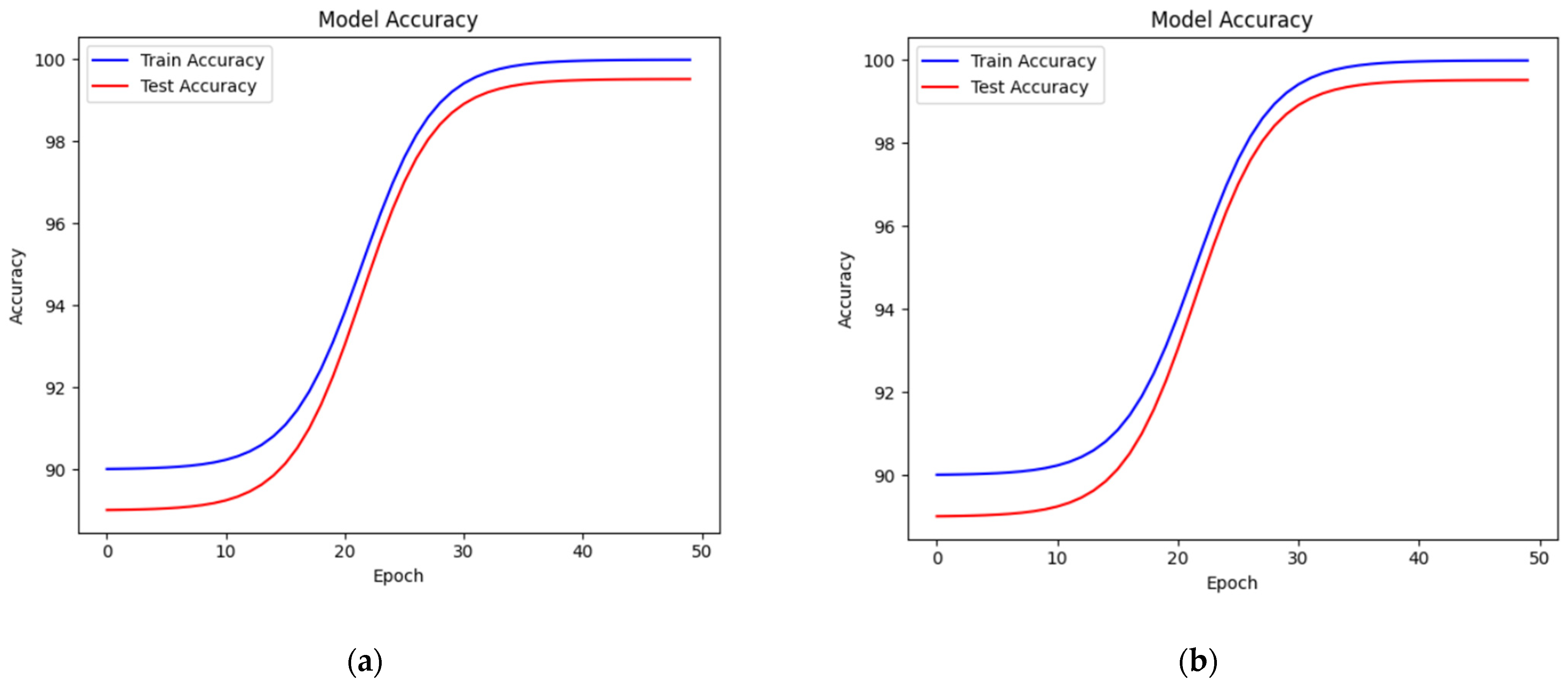
By examining the accuracy of the model in both the training and testing datasets, with and without noise, as shown in Figure 5a,b, it can be concluded that the model does not exhibit overfitting. The confusion matrix presented in Figure 6a demonstrates a remarkably consistent accuracy rate of 99.5% for all nine classes: normal, sag, swell, interruption, flicker, sag with harmonics, swell with harmonics, interruption with harmonics, and flicker with harmonics with a noiseless dataset. Each class exhibits only one incidence of misclassification, distributed among many categories, indicating that the classifier does not display a bias toward any given class, and its errors are not focused on particular misinterpretations. Overall, the classifier demonstrates a robust and balanced performance across all the classes. Despite the presence of noise in the dataset in Figure 6b, the classifier consistently maintains a high level of accuracy for all classes, with most classes obtaining a true positive rate of approximately 98.5%. Significantly, the misclassifications exhibit a slightly greater range, indicating the impact of noise. The interruption with harmonics class has a wider variety of misclassifications in comparison with the noiseless dataset. In general, despite the presence of noise, the classifier consistently demonstrates remarkable performance. However, certain classes such as interruption with harmonics and flicker with harmonics seem to be more vulnerable to errors caused by noise.
To obtain a more thorough evaluation of the efficacy of the proposed methodology, it was juxtaposed with recently proposed state-of-the-art methodologies. Table 4 displays the outcomes of the comparative analysis, particularly when subjected to significant levels of disruptive noise interference. The approaches discussed above exhibited notable degrees of precision. Nevertheless, it is important to acknowledge that the existing techniques have a very restricted range of categories related to PQ disturbance signals in contrast with the comprehensive model we have proposed. The DeepPQDS-FKTNet model achieved competitive performance in relation to the current leading approaches. The improved performance of DeepPQDS-FKTNet can be attributed to its bespoke design, which takes into consideration the intrinsic discriminative structures of PQDs. In contrast, other methods are manually constructed and do not rely on data-dependent approaches. The DeepPQDS-FKTNet-6 model has a commendable level of performance, with an accuracy rate of 98.5%. The utilization of an auto-deep-learning-based strategy, in conjunction with its capacity to effectively function in the presence of elevated levels of noise, renders it a resilient methodology. Although there may exist alternative approaches with marginally superior accuracy, it is noteworthy that DeepPQDS-FKTNet-6 exhibits a commendable performance. This is particularly impressive given the inherent difficulties associated with constructing an automated model derived from data including shallow architecture and high performance.

4. Conclusions

An automated technique was developed to generate a personalized deep learning model for PQD categorization. The FKT strategy was employed in order to construct a CNN model that was specifically designed for the target PQD dataset, taking into consideration the substantial number of parameters and random initialization often associated with CNN models. This approach was chosen to ensure the development of a cost-effective and efficient model with enhanced speed. To commence, the initial step involved the selection of the most representative PQD data through the utilization of the K-medoids clustering algorithm. Subsequently, Algorithm 1 was employed to choose appropriate kernels for the purpose of initializing the layers of the model. This facilitates the capture of more discriminative structures within the PQD dataset and allows for control over the depth of the model. The DeepPQDS-FKTNet model that was obtained exhibits a data-centric nature, characterized by a unique architectural design specifically tailored for the dataset. The DeepPQDS-FKTNet model demonstrates a comparable performance to state-of-the-art approaches in the PQD dataset while exhibiting a simpler complexity and parameter count. In subsequent research, we intend to augment DeepPQDS-FKTNet and tailor and incorporate our method into the transformer architecture in order to tackle the issue of energy forecasting while considering power quality disturbances (PQDs).

Author Contributions

Conceptualization, F.S. and S.A.; data curation, F.S., M.A., A.A.A.-S. and H.M.H.F.; formal analysis, F.S., S.A. and M.A.; funding acquisition and methodology, F.S. and A.A.A.-S.; project administration, H.M.H.F. and S.A.; resources, F.S. and S.A.; coding, F.S.; supervision, A.A.A.-S. and H.M.H.F.; validation, F.S.; visualization, F.S.; writing—original draft, F.S., All authors have read and agreed to the published version of the manuscript.

Funding

This work was supported and funded by the Deanship of Scientific Research at Imam Mohammad Ibn Saud Islamic University (IMSIU) (grant number IMSIU-RG23094).

Data Availability Statement

The data utilized to evaluate our algorithm was generated using open-source software specifically designed for generating synthetic power quality disruptions. It was created specifically for the purpose of evaluating different strategies for classifying power quality disturbances (PQD). The generated signals had a default duration of ten cycles, and the sampling rate for all signals was 3.2 kHz. The frequency was set to 50 Hz. The MATLAB 2016b software was utilized to construct the graphical user interface (GUI) and produce the corresponding code [28].

Conflicts of Interest

The authors declare no conflict of interest.

References

  1. Wang, C.; Ju, P.; Wu, F.; Pan, X.; Wang, Z. A systematic review on power system resilience from the perspective of generation, network, and load. Renew. Sustain. Energy Rev. 2022, 167, 112567. [Google Scholar] [CrossRef]
  2. Afonso, J.L.; Tanta, M.; Pinto, J.G.O.; Monteiro, L.F.C.; Machado, L.; Sousa, T.J.C.; Monteiro, V. A Review on Power Electronics Technologies for Power Quality Improvement. Energies 2021, 14, 8585. [Google Scholar] [CrossRef]
  3. Alam, M.R.; Bai, F.; Yan, R.; Saha, T.K. Classification and visualization of power quality disturbance-events using space vector ellipse in complex plane. IEEE Trans. Power Deliv. 2020, 36, 1380–1389. [Google Scholar] [CrossRef]
  4. Vazquez, S.; Zafra, E.; Aguilera, R.P.; Geyer, T.; Leon, J.I.; Franquelo, L.G. Prediction model with harmonic load current components for FCS-MPC of an uninterruptible power supply. IEEE Trans. Power Electron. 2021, 37, 322–331. [Google Scholar] [CrossRef]
  5. Sharma, A.; Rajpurohit, B.S.; Singh, S.N. A review on economics of power quality: Impact, assessment and mitigation. Renew. Sustain. Energy Rev. 2018, 88, 363–372. [Google Scholar] [CrossRef]
  6. Khaleel, M.; Abulifa, S.A.; Abulifa, A.A. Artificial Intelligent Techniques for Identifying the Cause of Disturbances in the Power Grid. Brill. Res. Artif. Intell. 2023, 3, 19–31. [Google Scholar] [CrossRef]
  7. Caicedo, J.E.; Agudelo-Martínez, D.; Rivas-Trujillo, E.; Meyer, J. A systematic review of real-time detection and classification of power quality disturbances. Prot. Control Mod. Power Syst. 2023, 8, 3. [Google Scholar] [CrossRef]
  8. Chawda, G.S.; Shaik, A.G.; Shaik, M.; Padmanaban, S.; Holm-Nielsen, J.B.; Mahela, O.P.; Kaliannan, P. Comprehensive Review on Detection and Classification of Power Quality Disturbances in Utility Grid with Renewable Energy Penetration. IEEE Access 2020, 8, 146807–146830. [Google Scholar] [CrossRef]
  9. Mishra, M.; Nayak, J.; Naik, B.; Abraham, A. Deep learning in electrical utility industry: A comprehensive review of a decade of research. Eng. Appl. Artif. Intell. 2020, 96, 104000. [Google Scholar] [CrossRef]
  10. Gunawan, T.S.; Husodo, B.Y.; Ihsanto, E.; Ramli, K. Power Quality Disturbance Classification Using Deep BiLSTM Architectures with Exponentially Decayed Number of Nodes in the Hidden Layers. In Recent Trends in Mechatronics Towards Industry 4.0: Selected Articles from iM3F 2020, Malaysia; Springer: Berlin/Heidelberg, Germany, 2022. [Google Scholar]
  11. Li, Z.; Liu, H.; Zhao, J.; Bi, T.; Yang, Q. A Power System Disturbance Classification Method Robust to PMU Data Quality Issues. IEEE Trans. Ind. Inform. 2021, 18, 130–142. [Google Scholar] [CrossRef]
  12. Eikeland, O.F.; Holmstrand, I.S.; Bakkejord, S.; Chiesa, M.; Bianchi, F.M. Detecting and Interpreting Faults in Vulnerable Power Grids with Machine Learning. IEEE Access 2021, 9, 150686–150699. [Google Scholar] [CrossRef]
  13. Hong, W.; Liu, Z.; Wu, X. Power quality disturbance recognition based on wavelet transform and convolutional neural network. In Proceedings of the 2021 IEEE International Conference on Artificial Intelligence and Computer Applications (ICAICA), Dalian, China, 28–30 June 2021; IEEE: Piscataway, NJ, USA, 2021. [Google Scholar]
  14. Li, J.; Liu, H.; Wang, D.; Bi, T. Classification of Power Quality Disturbance Based on S-Transform and Convolution Neural Network. Front. Energy Res. 2021, 9, 708131. [Google Scholar] [CrossRef]
  15. Zhang, Y.; Zhou, X. Classification of power quality disturbances using visual attention mechanism and feed-forward neural network. Measurement 2022, 188, 110390. [Google Scholar] [CrossRef]
  16. Reddy, K.R. Power quality classification of disturbances using discrete wavelet packet transform (DWPT) with adaptive neuro-fuzzy system. Turk. J. Comput. Math. Educ. TURCOMAT 2021, 12, 4892–4903. [Google Scholar]
  17. IEEE 1159-2009; IEEE Recommended Practice for Monitoring Electric Power Quality. IEEE: New York, NY, USA, 2009.
  18. Huo, X. A Statistical analysis of Fukunaga–Koontz transform. IEEE Signal Process. Lett. 2004, 11, 123–126. [Google Scholar] [CrossRef]
  19. Saeed, F.; Hussain, M.; Aboalsamh, H.A. Automatic Fingerprint Classification Using Deep Learning Technology (DeepFKTNet). Mathematics 2022, 10, 1285. [Google Scholar] [CrossRef]
  20. Saeed, F.; Hussain, M.; Aboalsamh, H.A. Method for Fingerprint Classification. U.S. Patent 9530042, 13 June 2016. [Google Scholar]
  21. Zhang, Q.; Couloigner, I. A new and efficient k-medoid algorithm for spatial clustering. In Proceedings of the International Conference on Computational Science and Its Applications, Singapore, 9–12 May 2005; Springer: Berlin/Heidelberg, Germany, 2005. [Google Scholar]
  22. Lin, M.; Chen, Q.; Yan, S. Network in network. arXiv 2013, arXiv:1312.4400. [Google Scholar]
  23. Rousseeuw, P.J. Silhouettes: A graphical aid to the interpretation and validation of cluster analysis. J. Comput. Appl. Math. 1987, 20, 53–65. [Google Scholar] [CrossRef]
  24. He, K.; Zhang, X.; Ren, S.; Sun, J. Deep residual learning for image recognition. In Proceedings of the IEEE Conference on Computer Vision and Pattern Recognition, Las Vegas, NV, USA, 27–30 June 2016. [Google Scholar]
  25. Huang, G.; Liu, Z.; Van Der Maaten, L.; Weinberger, K.Q. Densely connected convolutional networks. CVPR 2017. arXiv 2016, arXiv:1608.06993. [Google Scholar]
  26. Szegedy, C.; Liu, W.; Jia, Y.; Sermanet, P.; Reed, S.; Anguelov, D.; Erhan, D.; Vanhoucke, V.; Rabinovich, A. Going deeper with convolutions. In Proceedings of the IEEE Conference on Computer Vision and Pattern Recognition, Boston, MA, USA, 7–12 June 2015. [Google Scholar]
  27. Mika, S.; Ratsch, G.; Weston, J.; Scholkopf, B.; Mullers, K.R. Fisher discriminant analysis with kernels. In Neural Networks for Signal Processing IX: Proceedings of the 1999 IEEE Signal Processing Society Workshop (Cat. No. 98th8468); IEEE: Piscataway, NJ, USA, 1999. [Google Scholar]
  28. Machlev, R.; Chachkes, A.; Belikov, J.; Beck, Y.; Levron, Y. Open source dataset generator for power quality disturbances with deep-learning reference classifiers. Electr. Power Syst. Res. 2021, 195, 107152. [Google Scholar] [CrossRef]
  29. Cook, A. Global Average Pooling Layers for Object Localization. 2017. Available online: https://alexisbcook.github.io/2017/globalaverage-poolinglayers-for-object-localization/ (accessed on 19 August 2019).
  30. Akiba, T.; Sano, S.; Yanase, T.; Ohta, T.; Koyama, M. Optuna: A next-generation hyperparameter optimization framework. In Proceedings of the 25th ACM SIGKDD International Conference on Knowledge Discovery & Data Mining, Anchorage, AK, USA, 4–8 August 2019. [Google Scholar]
  31. Gao, Z.; Li, J.; Guo, J.; Chen, Y.; Yi, Z.; Zhong, J. Diagnosis of Diabetic Retinopathy Using Deep Neural Networks. IEEE Access 2018, 7, 3360–3370. [Google Scholar] [CrossRef]
  32. Quellec, G.; Charrière, K.; Boudi, Y.; Cochener, B.; Lamard, M. Deep image mining for diabetic retinopathy screening. Med. Image Anal. 2017, 39, 178–193. [Google Scholar] [CrossRef] [PubMed]
  33. Chowdhury, A.R.; Chatterjee, T.; Banerjee, S. A Random Forest classifier-based approach in the detection of abnormalities in the retina. Med. Biol. Eng. Comput. 2019, 57, 193–203. [Google Scholar] [CrossRef] [PubMed]
  34. Zhang, W.; Zhong, J.; Yang, S.; Gao, Z.; Hu, J.; Chen, Y.; Yi, Z. Automated identification and grading system of diabetic retinopathy using deep neural networks. Knowl. Based Syst. 2019, 175, 12–25. [Google Scholar] [CrossRef]
  35. Haghighi, S.; Jasemi, M.; Hessabi, S.; Zolanvari, A. PyCM: Multiclass confusion matrix library in Python. J. Open Source Softw. 2018, 3, 729. [Google Scholar] [CrossRef]
  36. Powers, D.M. Evaluation: From precision, recall and F-measure to ROC, informedness, markedness and correlation. arXiv 2011, arXiv:2010.16061. [Google Scholar]
  37. Fleiss, J.L.; Cohen, J.; Everitt, B.S. Large sample standard errors of kappa and weighted kappa. Psychol. Bull. 1969, 72, 323. [Google Scholar] [CrossRef]
  38. Li, J.; Teng, Z.; Tang, Q.; Song, J. Detection and classification of power quality disturbances using double resolution S-transform and DAG-SVMs. IEEE Trans. Instrum. Meas. 2016, 65, 2302–2312. [Google Scholar] [CrossRef]
  39. Qiu, W.; Tang, Q.; Liu, J.; Yao, W. An automatic identification framework for complex power quality disturbances based on multifusion convolutional neural network. IEEE Trans. Ind. Inform. 2019, 16, 3233–3241. [Google Scholar] [CrossRef]
  40. Liu, M.; Chen, Y.; Zhang, Z.; Deng, S. Classification of Power Quality Disturbance Using Segmented and Modified S-Transform and DCNN-MSVM Hybrid Model. IEEE Access 2023, 11, 890–899. [Google Scholar] [CrossRef]
  41. Mozaffari, M.; Doshi, K.; Yilmaz, Y. Real-Time Detection and Classification of Power Quality Disturbances. Sensors 2022, 22, 7958. [Google Scholar] [CrossRef] [PubMed]
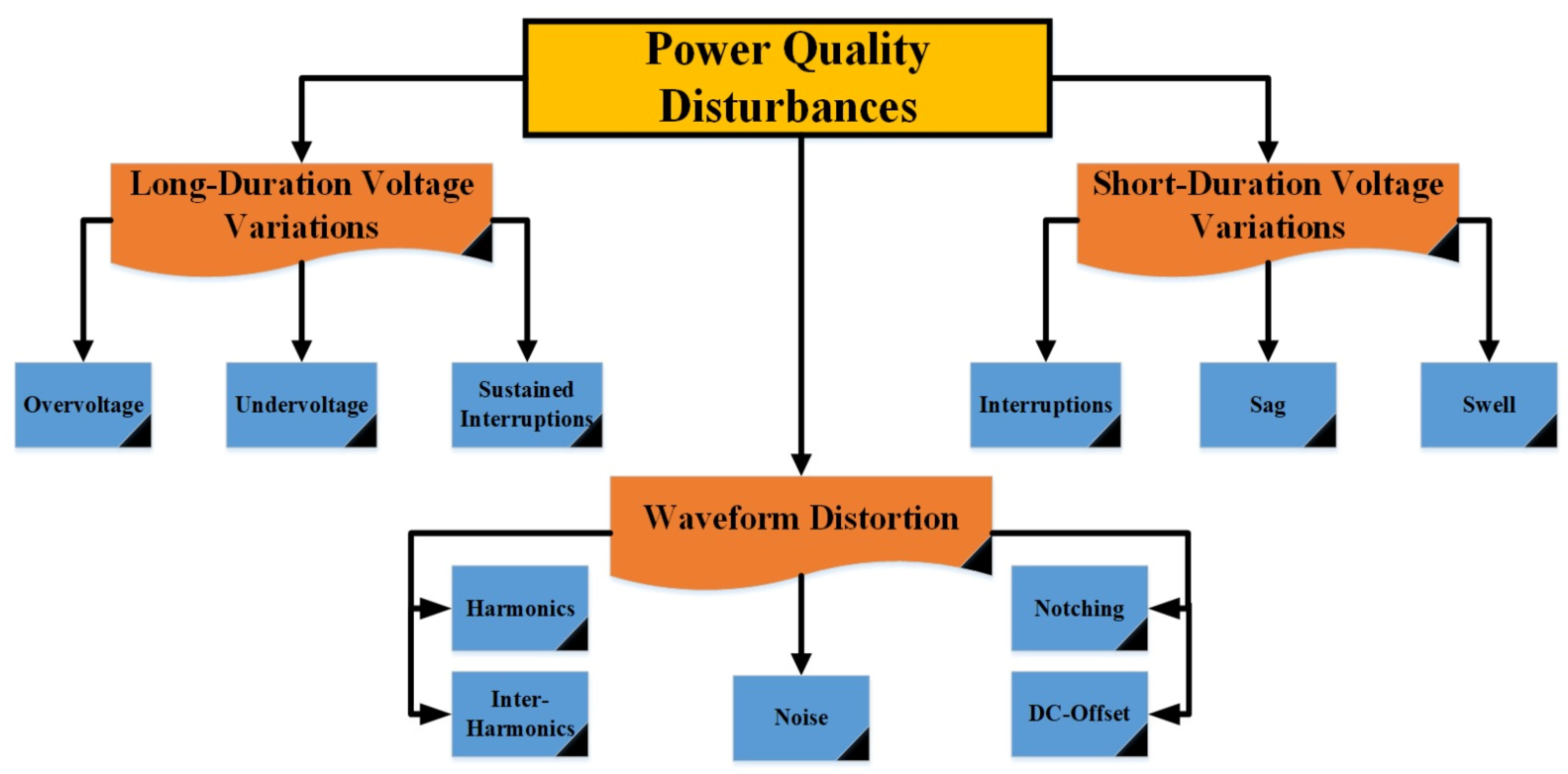
Figure 1. Power quality disturbance classification according to IEEE-1159 standard [17].
Mathematics 11 04726 g001
Figure 2. Design procedure of DeepPQDS-FKTNet; (a) The core architecture of DeepPQDS-FKTNet, and (b) global pooling and softmax layers are added to the model.
Mathematics 11 04726 g002
Figure 4. (a) FKTNET architecture for a noiseless synthetic dataset and (b) FKTNET architecture for a noisy synthetic dataset.
Mathematics 11 04726 g004
Figure 5. Train and test ACC for DeepPQDS-FKTNet model for (a) noiseless and (b) noisy synthetic PQDs.
Mathematics 11 04726 g005
Figure 6. Test confusion matrix for DeepPQDS-FKTNet model for (a) noiseless and (b) noisy synthetic PQDs.
Mathematics 11 04726 g006
Table 1. PQD mathematical models used by the synthetic generator: 9 types [28].
DisturbanceCharacteristics EquationParameters
1 Normal[1 ± α(u(t − t1) − u(t − t2))] sin(ωt)α < 0.4, T ≤ (t2 − t1) ≤ 9T
2 Sag[1 − α(u(t − t1) − u(t − t2))] sin(ωt)0.1 ≤ α < 0.9, T ≤ (t2 − t1) ≤ 9T
3 Swell[1 + α(u(t − t1) − u(t − t2))] sin(ωt)0.1 ≤ α ≤ 0.8, T ≤ (t2 − t1) ≤ 9T
4 Interruption[1 − α(u(t − t1) − u(t − t2))] sin(ωt)0.9 ≤ α ≤ 1, T ≤ (t2 − t1) ≤ 9T
5 Flicker[1 + αf sin(βωt)] sin(ωt)0.1 ≤ αf < 0.2, 5 ≤ β < 20 Hz
6 Sag with harmonics[1 − α(u(t − t1) − u(t − t2))] ×
1 sin(ωt) + α3 sin(3ωt) + α5 sin(5ωt) + α7 sin(7ωt)]
0.1 ≤ α ≤ 0.9, T ≤ (t2 − t1) ≤ 9T,
0.05 α 3 , α 5 , α 7 0.15 ,   α i 2 = 1
7 Swell with harmonics[1 + α(u(t − t1) − u(t − t2))] ×
1 sin(ωt) + α3 sin(3ωt) + α5 sin(5ωt) + α7 sin(7ωt)]
0.1 ≤ α ≤ 0.8, T ≤ (t2 − t1) ≤ 9T,
0.05 α 3 , α 5 , α 7 0.15 ,   α i 2 = 1
8 Interruption with harmonics[1 − α(u(t − t1) − u(t − t2))] ×
1 sin(ωt) + α3 sin(3ωt) + α5 sin(5ωt) + α7 sin(7ωt)]
0.9 ≤ α ≤ 1, T ≤ (t2 − t1) ≤ 9T,
0.05 α 3 , α 5 , α 7 0.15 ,   α i 2 = 1
9 Flicker with harmonics[1 + αf sin(βωt)] ×
1 sin(ωt) + α3 sin(3ωt) + α5 sin(5ωt) + α7 sin(7ωt)]
0.1 ≤ αf < 0.2, 5 ≤ β < 20,
0.05 α 3 , α 5 , α 7 0.15 ,   α i 2 = 1
Table 2. The optimized hyperparameters using Optuna algorithm.
DatasetActivation FunctionLearning RatePatch’s SizeOptimizerDropout
Synthetic dataset without noiseRelu60.0018RMSprop0.25
Synthetic dataset with noiseRelu60.00028RMSprop0.35
Table 3. Comparison between DeepPQDS-FKTNet models and the fine-tuned customized pre-trained models for noisy and noiseless synthetic PQDs. G, M, and K stand for giga, mega, and kilo.
DatasetModel# FLOPs# ParametersACC %SE %SP %Kappa %
NoiselessGoogleNet1.44 G7.3 M94.492.4196.6191.12
ResNet500.089 G0.64 M95.2392.8797.1290.82
DeepPQDS-FKTNet-50.003 G55.4 K99.5194.3898.1893.13
NoisyGoogleNet1.44 G7.3 M93.191.594.9991.12
ResNet500.089 G0.64 M94.1291.3895.3790.82
DeepPQDS-FKTNet-60.0035 G55.9 K98.593.9899.2892.43
Table 4. Comparison between DeepPQDS-FKTNet-6 and state-of-the-art methods.
PaperMethodNoise (dB)Number of PQDsACC (%)
Cai et al., 2019 [38] DRST + DAG + SVM20997.77
Qiu et al., 2019 [39]Multifusion convolutional neural network (MFCNN)-2499.26
Liu et al., 2023 [40]SMST + DCNN + MSVM202198.86
Mozaffari et al., 2022 [41]Vector-ODIT20
30

5
98.38
100
DeepPQDS-FKTNet-6FKTNet model (six layers and one softmax layer)50998.5
Disclaimer/Publisher’s Note: The statements, opinions and data contained in all publications are solely those of the individual author(s) and contributor(s) and not of MDPI and/or the editor(s). MDPI and/or the editor(s) disclaim responsibility for any injury to people or property resulting from any ideas, methods, instructions or products referred to in the content.