
Intelligent Classification and Diagnosis of Diabetes and Impaired Glucose Tolerance Using Deep Neural Networks


Abstract
:1. Introduction
- Serial data classification is performed using deep neural networks.
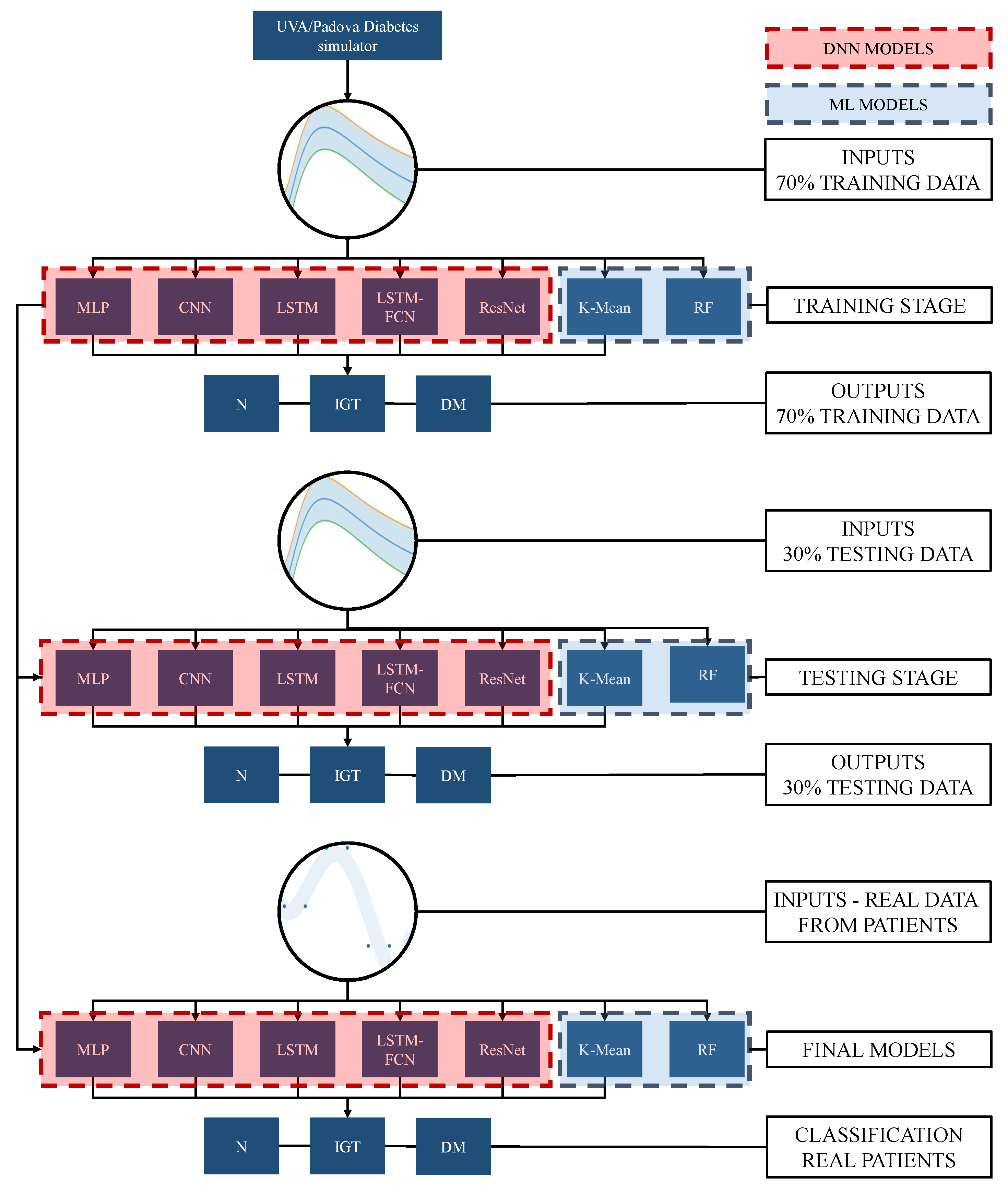
- Data from healthy patients, as well as patients with impaired glucose tolerance and with diabetes mellitus were generated by means of Dalla Man and UVA/Padova mathematical models.
- The classification performance of the proposed deep neural networks is compared.
- The neural classifiers are validated with serial data from real patients.
2. Methodology
3. Deep Neuronal Network for Time Series Classification
3.1. Time Series Classification
3.2. Deep Neural Networks
3.3. Multilayer Perceptron Neural Networks
3.4. Convolutional Neural Network
3.5. Long Short-Term Memory Recurrent Neural Network
3.6. LSTM Fully Convolutional Networks
3.7. Residual Deep Networks
4. Machine Learning Models
4.1. Random Forest
4.2. K-Means
5. Oral Glucose Tolerance Test
- OGTT recognizes altered postprandial metabolism, making it a method capable of detecting diabetes more efficiently than plasma glucose concentration and overnight fasting (FPG).
- An altered fasting blood glucose (IFG) has a normal 2hPG established by OGTT.
- FPG does not provide relevant metabolic information.
6. Simulated Data Acquisition
7. Real Data Description
8. Results
9. Conclusions
Author Contributions
Funding
Data Availability Statement
Acknowledgments
Conflicts of Interest
Appendix A
Appendix A.1. Real Patients Data
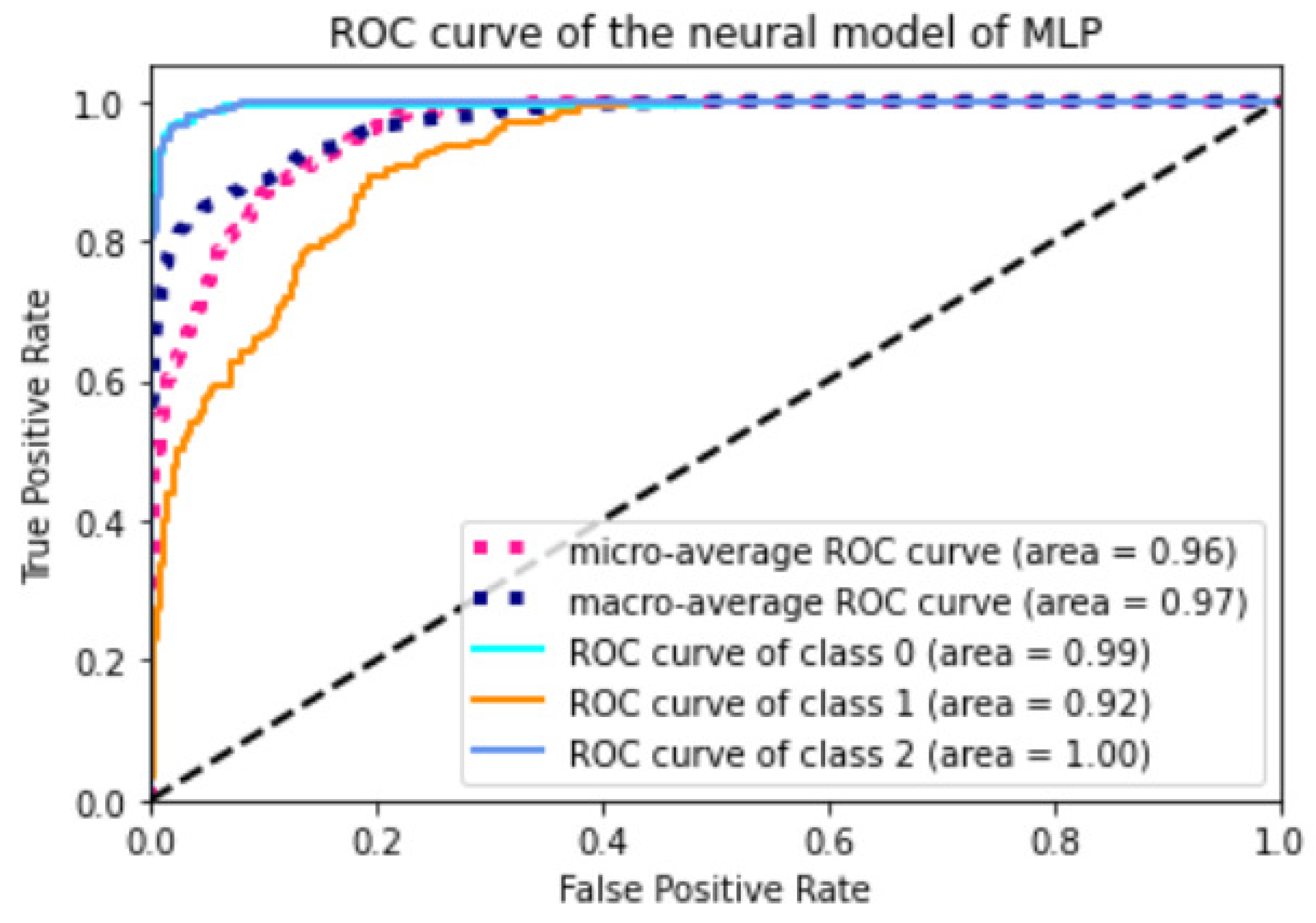
Appendix A.2. Models ROC Curves


References
- Stuart, P.J.; Crooks, S.; Porton, M. An interventional program for diagnostic testing in the emergency department. Med. J. Aust. 2002, 177, 131–134. [Google Scholar] [CrossRef] [PubMed]
- Pölsterl, S.; Conjeti, S.; Navab, N.; Katouzian, A. Survival analysis for high-dimensional, heterogeneous medical data: Exploring feature extraction as an alternative to feature selection. Artif. Intell. Med. 2016, 72, 1–11. [Google Scholar] [CrossRef] [PubMed]
- Kumar, D.; Jain, N.; Khurana, A.; Mittal, S.; Satapathy, S.C.; Senkerik, R.; Hemanth, J.D. Automatic detection of white blood cancer from bone marrow microscopic images using convolutional neural networks. IEEE Access 2020, 8, 142521–142531. [Google Scholar] [CrossRef]
- Javeed, A.; Zhou, S.; Yongjian, L.; Qasim, I.; Noor, A.; Nour, R. An intelligent learning system based on random search algorithm and optimized random forest model for improved heart disease detection. IEEE Access 2019, 7, 180235–180243. [Google Scholar] [CrossRef]
- Kulkarni, N.N.; Bairagi, V.K. Extracting salient features for EEG-based diagnosis of Alzheimer’s disease using support vector machine classifier. IETE J. Res. 2017, 63, 11–22. [Google Scholar] [CrossRef]
- Kumari, V.A.; Chitra, R. Classification of diabetes disease using support vector machine. Int. J. Eng. Res. Appl. 2013, 3, 1797–1801. [Google Scholar]
- Uchida, T.; Kanamori, T.; Teramoto, T.; Nonaka, Y.; Tanaka, H.; Nakamura, S.; Murayama, N. Identifying Glucose Metabolism Status in Nondiabetic Japanese Adults Using Machine Learning Model with Simple Questionnaire. Comput. Math. Methods Med. 2022, 2022, 1026121. [Google Scholar] [CrossRef] [PubMed]
- Sejnowski, T.J.; Rosenberg, C.R. Parallel networks that learn to pronounce English text. Complex Syst. 1987, 1, 145–168. [Google Scholar]
- Zaremba, W.; Sutskever, I.; Vinyals, O. Recurrent neural network regularization. arXiv 2014, arXiv:1409.2329. [Google Scholar]
- Verner, A.; Mukherjee, S. An LSTM-Based Method for Detection and Classification of Sensor Anomalies. In Proceedings of the 2020 5th International Conference on Machine Learning Technologies, Beijing, China, 19–21 June 2020; pp. 39–45. [Google Scholar]
- Lee, X.Y.; Kumar, A.; Vidyaratne, L.; Rao, A.R.; Farahat, A.; Gupta, C. An ensemble of convolution-based methods for fault detection using vibration signals. arXiv 2023, arXiv:2305.05532. [Google Scholar]
- Oh, S.L.; Hagiwara, Y.; Raghavendra, U.; Yuvaraj, R.; Arunkumar, N.; Murugappan, M.; Acharya, U.R. A deep learning approach for Parkinson’s disease diagnosis from EEG signals. Neural Comput. Appl. 2020, 32, 10927–10933. [Google Scholar] [CrossRef]
- Maragatham, G.; Devi, S. LSTM model for prediction of heart failure in big data. J. Med Syst. 2019, 43, 111. [Google Scholar] [CrossRef] [PubMed]
- Sheng, B.; Chen, X.; Li, T.; Ma, T.; Yang, Y.; Bi, L.; Zhang, X. An overview of artificial intelligence in diabetic retinopathy and other ocular diseases. Front. Public Health 2022, 10, 971943. [Google Scholar] [CrossRef] [PubMed]
- Nomura, A.; Noguchi, M.; Kometani, M.; Furukawa, K.; Yoneda, T. Artificial intelligence in current diabetes management and prediction. Curr. Diabetes Rep. 2021, 21, 61. [Google Scholar] [CrossRef]
- Contreras, I.; Vehi, J. Artificial intelligence for diabetes management and decision support: Literature review. J. Med. Internet Res. 2018, 20, e10775. [Google Scholar] [CrossRef] [PubMed]
- Chaki, J.; Ganesh, S.T.; Cidham, S.; Theertan, S.A. Machine learning and artificial intelligence based Diabetes Mellitus detection and self-management: A systematic review. J. King Saud. Univ.-Comput. Inf. Sci. 2022, 34, 3204–3225. [Google Scholar] [CrossRef]
- Association, A.D. Classification and diagnosis of diabetes: Standards of Medical Care in Diabetes—2020. Diabetes Care 2020, 43, S14–S31. [Google Scholar] [CrossRef] [PubMed]
- Nathan, D.M.; Group, D.R. The diabetes control and complications trial/epidemiology of diabetes interventions and complications study at 30 years: Overview. Diabetes Care 2014, 37, 9–16. [Google Scholar] [CrossRef]
- Punthakee, Z.; Goldenberg, R.; Katz, P. Definition, classification and diagnosis of diabetes, prediabetes and metabolic syndrome. Can. J. Diabetes 2018, 42, S10–S15. [Google Scholar] [CrossRef]
- Association, A.D. Guide to Diagnosis and Classification of Diabetes Mellitus and Other Categories of Glucose Intolerance. Diabetes Care 1997, 20, S21. [Google Scholar] [CrossRef]
- Bello-Chavolla, O.Y.; Rojas-Martinez, R.; Aguilar-Salinas, C.A.; Hernández-Avila, M. Epidemiology of diabetes mellitus in Mexico. Nutr. Rev. 2017, 75, 4–12. [Google Scholar] [CrossRef] [PubMed]
- Martínez Basila, A.; Maldonado Hernández, J.; López Alarcón, M. Métodos diagnósticos de la resistencia a la insulina en la población pediátrica. Boletín Méd. Hosp. Infant. México 2011, 68, 397–404. [Google Scholar]
- Jia, F.; Lei, Y.; Lin, J.; Zhou, X.; Lu, N. Deep neural networks: A promising tool for fault characteristic mining and intelligent diagnosis of rotating machinery with massive data. Mech. Syst. Signal Process. 2016, 72, 303–315. [Google Scholar] [CrossRef]
- Ogunmolu, O.; Gu, X.; Jiang, S.; Gans, N. Nonlinear systems identification using deep dynamic neural networks. arXiv 2016, arXiv:1610.01439. [Google Scholar]
- Loh, H.W.; Ooi, C.P.; Palmer, E.; Barua, P.D.; Dogan, S.; Tuncer, T.; Baygin, M.; Acharya, U.R. GaborPDNet: Gabor transformation and deep neural network for Parkinson’s disease detection using EEG signals. Electronics 2021, 10, 1740. [Google Scholar] [CrossRef]
- Zhai, X.; Ali, A.A.S.; Amira, A.; Bensaali, F. MLP neural network based gas classification system on Zynq SoC. IEEE Access 2016, 4, 8138–8146. [Google Scholar] [CrossRef]
- Lim, T.Y.; Ratnam, M.M.; Khalid, M.A. Automatic classification of weld defects using simulated data and an MLP neural network. Insight-Non Test. Cond. Monit. 2007, 49, 154–159. [Google Scholar] [CrossRef]
- Girshick, R.; Donahue, J.; Darrell, T.; Malik, J. Rich feature hierarchies for accurate object detection and semantic segmentation. In Proceedings of the IEEE Conference on Computer Vision and Pattern Recognition, Columbus, OH, USA, 23–28 June 2014; pp. 580–587. [Google Scholar]
- Zheng, Y.; Liu, Q.; Chen, E.; Ge, Y.; Zhao, J.L. Time series classification using multi-channels deep convolutional neural networks. In Web-Age Information Management. WAIM 2014. Lecture Notes in Computer Science; Li, F., Li, G., Hwang, S.W., Yao, B., Zhang, Z., Eds.; Springer: Cham, Switzerland, 2014; pp. 298–310. [Google Scholar]
- Krizhevsky, A.; Sutskever, I.; Hinton, G.E. Imagenet classification with deep convolutional neural networks. Adv. Neural Inf. Process. Syst. 2012, 25, 1097–1105. [Google Scholar] [CrossRef]
- Albawi, S.; Bayat, O.; Al-Azawi, S.; Ucan, O.N. Social touch gesture recognition using convolutional neural network. Comput. Intell. Neurosci. 2018, 2018, 1881. [Google Scholar] [CrossRef]
- Hochreiter, S.; Schmidhuber, J. Long short-term memory. Neural Comput. 1997, 9, 1735–1780. [Google Scholar] [CrossRef]
- Siami-Namini, S.; Tavakoli, N.; Namin, A.S. The performance of LSTM and BiLSTM in forecasting time series. In Proceedings of the 2019 IEEE International Conference on Big Data (Big Data), Los Angeles, CA, USA, 9–12 December 2019; pp. 3285–3292. [Google Scholar] [CrossRef]
- Koley, B.; Dey, D. An ensemble system for automatic sleep stage classification using single channel EEG signal. Comput. Biol. Med. 2012, 42, 1186–1195. [Google Scholar] [CrossRef] [PubMed]
- Karim, F.; Majumdar, S.; Darabi, H.; Chen, S. LSTM fully convolutional networks for time series classification. IEEE Access 2017, 6, 1662–1669. [Google Scholar] [CrossRef]
- Kim, Y.; Sa, J.; Chung, Y.; Park, D.; Lee, S. Resource-efficient pet dog sound events classification using LSTM-FCN based on time-series data. Sensors 2018, 18, 4019. [Google Scholar] [CrossRef] [PubMed]
- He, K.; Zhang, X.; Ren, S.; Sun, J. Deep residual learning for image recognition. In Proceedings of the IEEE Conference on Computer Vision and Pattern Recognition, Las Vegas, NV, USA, 27–30 June 2016; pp. 770–778. [Google Scholar]
- Russakovsky, O.; Deng, J.; Su, H.; Krause, J.; Satheesh, S.; Ma, S.; Huang, Z.; Karpathy, A.; Khosla, A.; Bernstein, M.; et al. Imagenet large scale visual recognition challenge. Int. J. Comput. Vis. 2015, 115, 211–252. [Google Scholar] [CrossRef]
- Lin, T.Y.; Maire, M.; Belongie, S.; Hays, J.; Perona, P.; Ramanan, D.; Dollár, P.; Zitnick, C.L. Microsoft coco: Common objects in context. In Computer Vision – ECCV 2014. ECCV 2014. Lecture Notes in Computer Science; Fleet, D., Pajdla, T., Schiele, B., Tuytelaars, T., Eds.; Springer: Cham, Switzerland, 2014; pp. 740–755. [Google Scholar]
- Ferrandez, S.M.; Harbison, T.; Weber, T.; Sturges, R.; Rich, R. Optimization of a truck-drone in tandem delivery network using k-means and genetic algorithm. J. Ind. Eng. Manag. (JIEM) 2016, 9, 374–388. [Google Scholar] [CrossRef]
- Shan, P. Image segmentation method based on K-mean algorithm. EURASIP J. Image Video Process. 2018, 2018, 68. [Google Scholar] [CrossRef]
- Köbberling, J.; Berninger, D. Natural History of Glucose Tolerance in Relatives of Diabetic Patients: Low Prognostic Value of the Oral Glucose Tolerance Test. Diabetes Care 1980, 3, 21–26. [Google Scholar] [CrossRef] [PubMed]
- Kuo, F.Y.; Cheng, K.C.; Li, Y.; Cheng, J.T. Oral glucose tolerance test in diabetes, the old method revisited. World J. Diabetes 2021, 12, 786. [Google Scholar] [CrossRef]
- Pollak, F.; Araya, V.; Lanas, A.; Sapunar, J.; Arrese, M.; Aylwin, C.G.; Bezanilla, C.G.; Carrasco, E.; Carrasco, F.; Codner, E.; et al. II Consenso de la Sociedad Chilena de Endocrinología y Diabetes sobre resistencia a la insulina. Rev. Méd. Chile 2015, 143, 627–636. [Google Scholar] [CrossRef]
- Bailes, B.K. Diabetes Mellitus and its Chronic Complications. AORN J. 2002, 76, 265–282. [Google Scholar] [CrossRef]
- Dalla Man, C.; Rizza, R.A.; Cobelli, C. Meal simulation model of the glucose-insulin system. IEEE Trans. Biomed. Eng. 2007, 54, 1740–1749. [Google Scholar] [CrossRef] [PubMed]
- Man, C.D.; Micheletto, F.; Lv, D.; Breton, M.; Kovatchev, B.; Cobelli, C. The UVA/PADOVA type 1 diabetes simulator: New features. J. Diabetes Sci. Technol. 2014, 8, 26–34. [Google Scholar] [CrossRef] [PubMed]
- Visentin, R.; Dalla Man, C.; Cobelli, C. One-day Bayesian cloning of type 1 diabetes subjects: Toward a single-day UVA/Padova type 1 diabetes simulator. IEEE Trans. Biomed. Eng. 2016, 63, 2416–2424. [Google Scholar] [CrossRef] [PubMed]
- Sánchez, O.D.; Ruiz-Velázquez, E.; Alanís, A.Y.; Quiroz, G.; Torres-Treviño, L. Parameter estimation of a meal glucose–insulin model for TIDM patients from therapy historical data. IET Syst. Biol. 2019, 13, 8–15. [Google Scholar] [CrossRef] [PubMed]
- Group, N.D.D. Classification and diagnosis of diabetes mellitus and other categories of glucose intolerance. Diabetes 1979, 28, 1039–1057. [Google Scholar]
- Kuschinski, N.; Christen, J.A.; Monroy, A.; Alavez, S. Modeling oral glucose tolerance test (ogtt) data and its bayesian inverse problem. arXiv 2016, arXiv:1601.04753. [Google Scholar]
- Cerda, J.; Cifuentes, L. Uso de curvas ROC en investigación clínica: Aspectos teórico-prácticos. Rev. Chil. Infectología 2012, 29, 138–141. [Google Scholar] [CrossRef]


| Diabetes Mellitus in Nonpregnant Adult | ||
|---|---|---|
| Fasting value: | -h, 1-h, or 1 -h OGTT: | 2-h OGTT: |
| venous plasma ≥ 140 mg/dL (7.8 mmol/L) | venous plasma ≥ 200 mg/dL (11.1 mmol/L) | |
| venous whole blood ≥ 120 mg/dL (6.7 mmol/L) | venous whole blood ≥ 180 mg/dL (10.0 mmol/L) | |
| capillary whole blood ≥ 120 mg/dL (6.7 mmol/L) | capillary whole blood ≥ 120 mg/dL (6.7 mmol/L) | |
| Impaired Glucose Tolerance (IGT) in Nonpregnant Adults | ||
| Fasting value: | h, 1 h, or 1 h OGTT: | 2 h OGTT: |
| venous plasma < 140 mg/dL (7.8 mmol/L) | venous plasma ≥ 200 mg/dL (11.1 mmol/L) | venous plasma of between 140 and 200 mg/dL |
| (7.8 and 11.1 mmol/L) | ||
| venous whole blood < 120 mg/dL (6.7 mmol/L) | venous whole blood ≥ 180 mg/dL (10.0 mmol/L) | venous whole blood of between 120 and 180 mg/dL |
| (6.7 and 10.0 mmol/L) | ||
| capillary whole blood < 120 mg/dL (6.7 mmol/L) | capillary whole blood ≥ 200 mg/dL (11.1 mmol/L) | capillary whole blood of between 140 and 200 mg/dL) |
| (7.8 and 11.1 mmol/L) | ||
| Normal Glucose Levels in Nonpregnant Adults | ||
| Fasting value: | h, 1 h, or 1 -h OGTT: | 2 h OGTT: |
| venous plasma < 115 mg/dL (6.4 mmol/L) | venous plasma < 200 mg/dL (11.1 mmol/L) | venous plasma < 140 mg/dL (7.8 mmol/L) |
| venous whole blood < 100 mg/dL (5.6 mmol/L) | venous whole blood < 180 mg/dL (10.0 mmol/L) | venous whole blood < 120 mg/dL (6.7 mmol/L) |
| capillary whole blood < 100 mg/dL (100 mmol/L) | capillary whole blood < 200 mg/dL (11.1 mmol/L) | capillary whole blood < 140 mg/dL (7.8 mmol/L) |
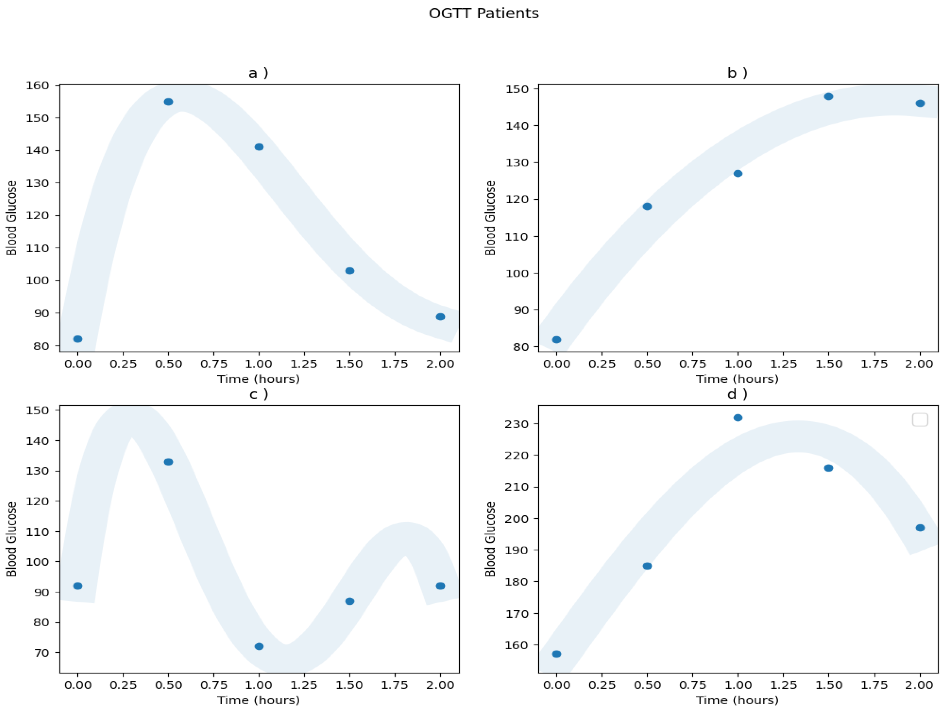
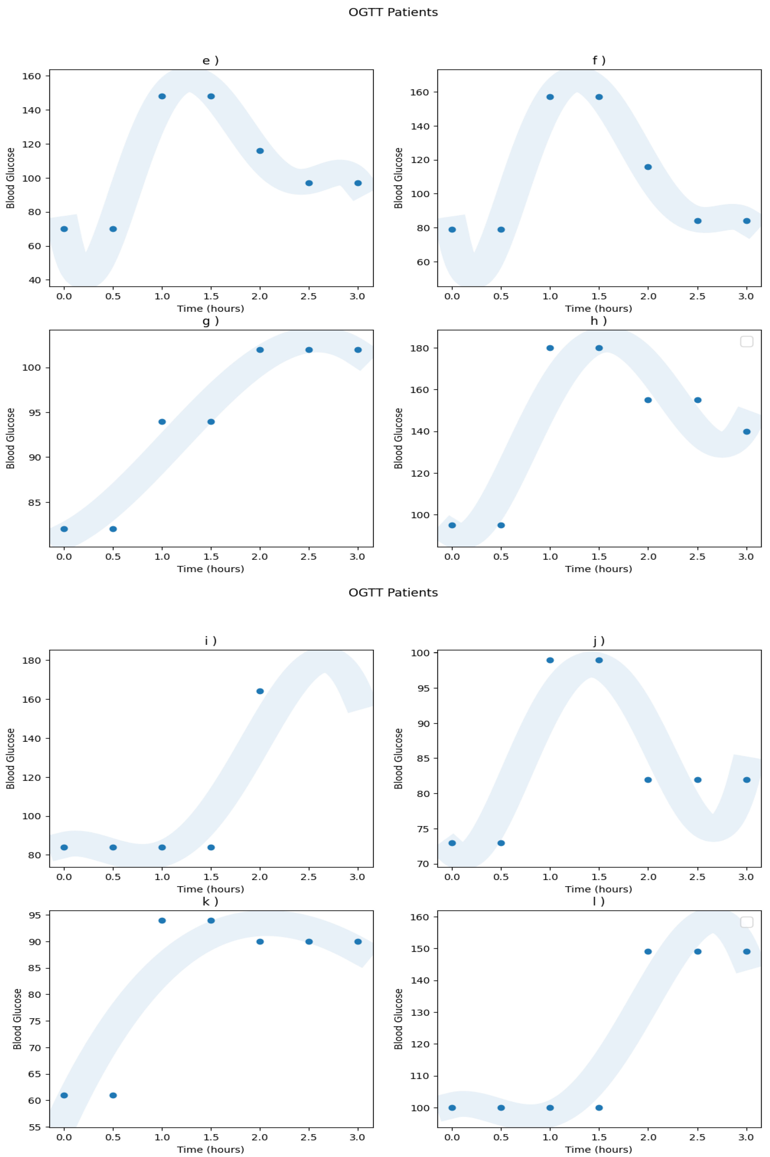
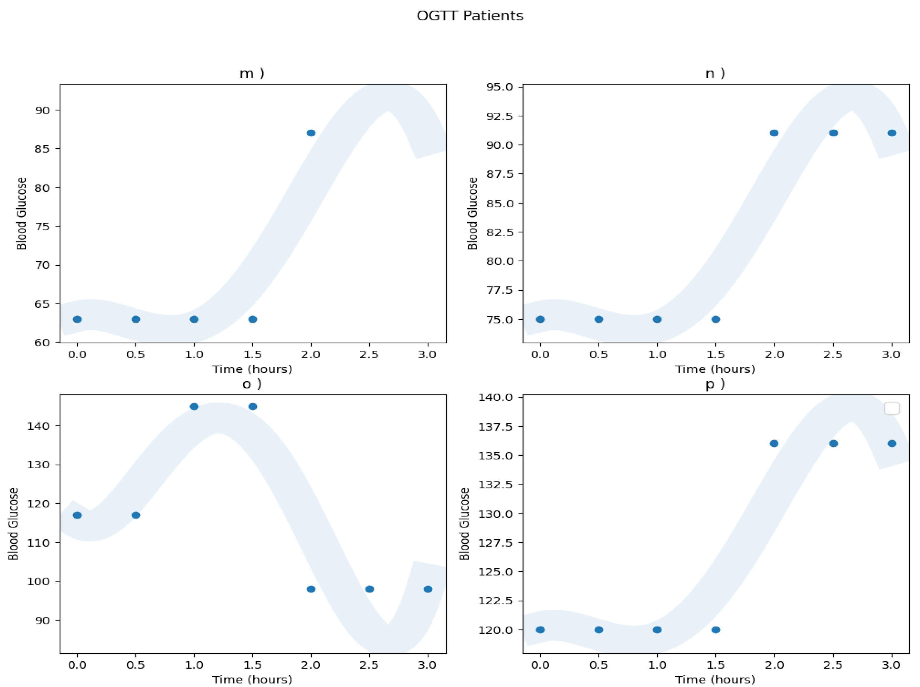
| Patient | a) | b) | c) | d) | e) | f) | g) | h) | i) | j) | k) | l) | m) | n) | o) | p) |
| Diagnosis | N | IGT | N | DM | N | N | N | IGT | IGT | N | N | IGT | N | N | IGT | IGT |
| Model | Class | AUC | CA | P(%) | R(%) | F1-Score |
|---|---|---|---|---|---|---|
| MLP | Normal | 0.99 | 0.96121 | 0.99218 | 0.94074 | 0.96577 |
| IGT | 0.99 | 0.96121 | 0.96323 | 0.95272 | 0.95795 | |
| Diabetes Mellitus | 1 | 0.96121 | 0.93782 | 0.98907 | 0.96276 | |
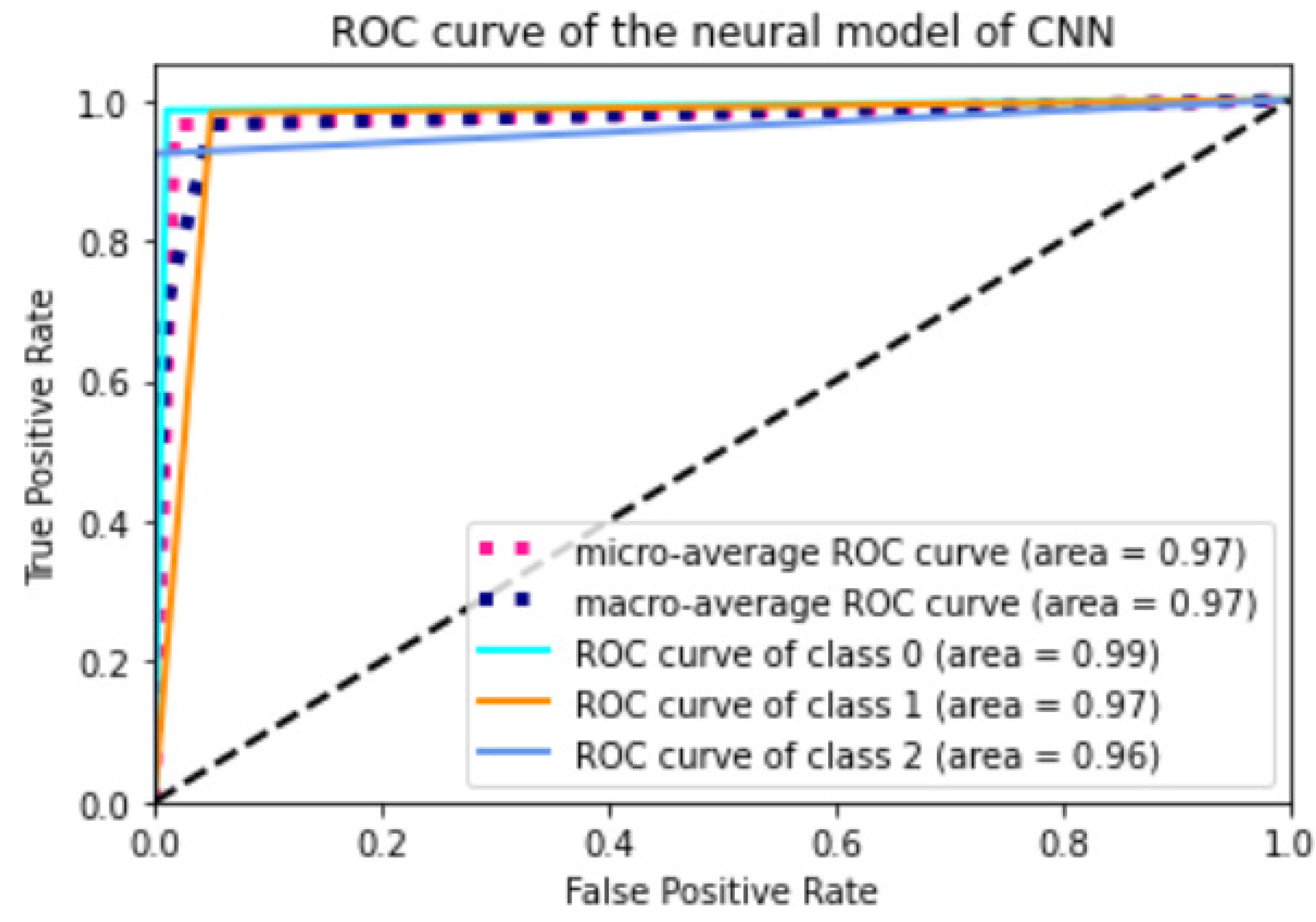
| CNN | Normal | 0.97 | 0.96795 | 0.97777 | 0.97777 | 0.97777 |
| IGT | 0.97 | 0.96795 | 0.94755 | 0.98545 | 0.96613 | |
| Diabetes Mellitus | 0.97 | 0.96795 | 0.99418 | 0.93442 | 0.96338 | |
| LSTM | Normal | 0.96 | 0.96290 | 0.94029 | 0.93333 | 0.93680 |
| IGT | 0.96 | 0.96290 | 0.96691 | 0.95636 | 0.96160 | |
| Diabetes Mellitus | 0.99 | 0.96290 | 0.97326 | 0.99453 | 0.98378 | |
| LSTM-FCN | Normal | 0.99 | 0.95784 | 1 | 0.92592 | 0.96153 |
| IGT | 0.99 | 0.95784 | 0.94014 | 0.97090 | 0.95527 | |
| Diabetes | 1 | 0.95784 | 0.95652 | 0.96174 | 0.95912 | |
| ResNet | Normal | 0.99 | 0.93591 | 0.99206 | 0.92592 | 0.95785 |
| IGT | 0.94 | 0.93591 | 0.94382 | 0.91636 | 0.92988 | |
| Diabetes Mellitus | 0.94 | 0.93591 | 0.89 | 0.97267 | 0.92950 | |
| K-Means | Normal | 0.93 | 0.925 | 0.88095 | 0.90243 | 0.89156 |
| IGT | 0.93 | 0.925 | 0.93548 | 0.90625 | 0.92063 | |
| Diabetes Mellitus | 0.96 | 0.925 | 0.93846 | 0.96825 | 0.95312 | |
| RF | Normal | 1 | 0.97 | 1 | 0.97560 | 0.98765 |
| IGT | 0.97 | 0.97 | 0.96875 | 0.96875 | 0.96875 | |
| Diabetes Mellitus | 0.97 | 0.97 | 0.95312 | 0.96825 | 0.96062 |
| Model | MLP | CNN | LSTM | LSTM-FCN | ResNet | K-Means | RF |
|---|---|---|---|---|---|---|---|
| Patient | Diagnosis | ||||||
| a) | N | N | N | N | N | N | N |
| b) | N | IGT | IGT | IGT | IGT | IGT | IGT |
| c) | N | N | N | N | N | N | N |
| d) | DM | DM | DM | DM | DM | DM | DM |
| e) | IGT | N | N | DM | N | N | N |
| f) | IGT | IGT | N | DM | N | IGT | N |
| g) | N | N | N | N | N | N | N |
| h) | IGT | IGT | IGT | DM | IGT | IGT | IGT |
| i) | N | DM | IGT | DM | DM | IGT | N |
| j) | N | N | N | N | N | N | N |
| k) | N | N | N | N | N | N | N |
| l) | N | IGT | IGT | DM | IGT | IGT | IGT |
| m) | N | N | N | N | N | N | N |
| n) | N | N | N | N | N | N | N |
| o) | N | IGT | N | DM | IGT | N | IGT |
| p) | IGT | IGT | IGT | IGT | IGT | IGT | IGT |
| Model | Class | CA | P(%) | R(%) | F1-Score |
|---|---|---|---|---|---|
| MLP | Normal | 0.82967 | 0.75280 | 0.99259 | 0.7 |
| IGT | 0.82967 | 0.80208 | 0.84 | 0.4 | |
| Diabetes Mellitus | 0.82967 | 1 | 0.69398 | 1 | |
| CNN | Normal | 0.96458 | 0.96376 | 0.98518 | 0.94117 |
| IGT | 0.96458 | 0.94405 | 0.98181 | 0.83333 | |
| Diabetes Mellitus | 0.96458 | 1 | 0.92349 | 0.66666 | |
| LSTM | Normal | 0.96121 | 0.94696 | 0.92592 | 0.94736 |
| IGT | 0.96121 | 0.95985 | 0.95636 | 0.90909 | |
| Diabetes Mellitus | 0.96121 | 0.97326 | 0.99453 | 1 | |
| LSTM-FCN | Normal | 0.96121 | 0.99230 | 0.95555 | 0.875 |
| IGT | 0.96121 | 0.94366 | 0.97454 | 0.5 | |
| Diabetes Mellitus | 0.96121 | 0.96648 | 0.94535 | 0.25 | |
| ResNet | Normal | 0.82967 | 0.85517 | 0.91851 | 1 |
| IGT | 0.82967 | 0.95360 | 0.67272 | 0.90909 | |
| Diabetes Mellitus | 0.82967 | 0.72047 | 1 | 0.66666 | |
| K-Means | Normal | 0.875 | 0.8888 | 0.8888 | 0.8888 |
| IGT | 0.875 | 0.8333 | 0.8333 | 0.8333 | |
| Diabetes Mellitus | 0.875 | 1 | 1 | 1 | |
| RF | Normal | 0.9375 | 1 | 0.9360 | 0.9 |
| IGT | 0.9375 | 0.8333 | 0.9473 | 0.8 | |
| Diabetes Mellitus | 0.9375 | 1 | 1 | 1 |
Disclaimer/Publisher’s Note: The statements, opinions and data contained in all publications are solely those of the individual author(s) and contributor(s) and not of MDPI and/or the editor(s). MDPI and/or the editor(s) disclaim responsibility for any injury to people or property resulting from any ideas, methods, instructions or products referred to in the content. |
© 2023 by the authors. Licensee MDPI, Basel, Switzerland. This article is an open access article distributed under the terms and conditions of the Creative Commons Attribution (CC BY) license (https://creativecommons.org/licenses/by/4.0/).
Share and Cite
Alanis, A.Y.; Sanchez, O.D.; Vaca-González, A.; Rangel-Heras, E. Intelligent Classification and Diagnosis of Diabetes and Impaired Glucose Tolerance Using Deep Neural Networks. Mathematics 2023, 11, 4065. https://doi.org/10.3390/math11194065
Alanis AY, Sanchez OD, Vaca-González A, Rangel-Heras E. Intelligent Classification and Diagnosis of Diabetes and Impaired Glucose Tolerance Using Deep Neural Networks. Mathematics. 2023; 11(19):4065. https://doi.org/10.3390/math11194065
Chicago/Turabian StyleAlanis, Alma Y., Oscar D. Sanchez, Alonso Vaca-González, and Eduardo Rangel-Heras. 2023. "Intelligent Classification and Diagnosis of Diabetes and Impaired Glucose Tolerance Using Deep Neural Networks" Mathematics 11, no. 19: 4065. https://doi.org/10.3390/math11194065
APA StyleAlanis, A. Y., Sanchez, O. D., Vaca-González, A., & Rangel-Heras, E. (2023). Intelligent Classification and Diagnosis of Diabetes and Impaired Glucose Tolerance Using Deep Neural Networks. Mathematics, 11(19), 4065. https://doi.org/10.3390/math11194065