


Convergence of the Euler Method for Impulsive Neutral Delay Differential Equations


Abstract
1. Introduction
2. Main Result
3. Examples
3.1. Example 1
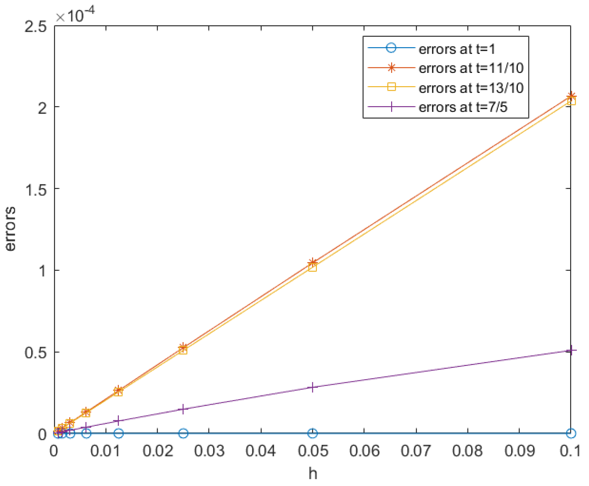
3.2. Example 2
4. Conclusions
Author Contributions
Funding
Data Availability Statement
Conflicts of Interest
References
- Bellen, A.; Guglielmi, N.; Zennaro, M. Numerical stability of nonlinear delay differential equations of neutral type. J. Comput. Appl. Math. 2000, 125, 251–263. [Google Scholar] [CrossRef]
- Hu, G.; Hu, G.; Cahlon, B. Algebraic criteria for stability of linear neutral systems with a single delay. J. Comput. Appl. Math. 2001, 135, 125–133. [Google Scholar] [CrossRef]
- Dugard, L.; Verriest, E.I. (Eds.) Stability and Control of Time Delay Systems; Springer: London, UK, 1998. [Google Scholar]
- Gorechi, H.; Fuksa, S.; Grabowski, P.; Korytowski, A. Analysis and Synthesis of Time Delay Systems; PWN: Warsaw, Poland, 1989. [Google Scholar]
- Kolmanovskii, V.B.; Myshkis, A. Applied Theory of Functional Differential Equations; Kluwer Academic Publishers: Dordrecht, The Netherlands, 1992. [Google Scholar]
- Gopalsamy, K. Stability and Oscillations in Delay Differential Equations of Population Dynamics; Kluwer Academic Publishers: Boston, MA, USA, 1992. [Google Scholar]
- Sinha, A.S.C.; El-Sharkawy, M.A.; Rizkalla, M.; Suzuki, D.A. A constructive algorithm for stabilization of nonlinear neutral time-delayed systems occurring in bioengineering. Int. J. Syst. Sci. 1996, 27, 17–25. [Google Scholar] [CrossRef]
- Park, J.H.; Kwon, O.; Lee, S. State estimation for neural networks of neutral-type with interval time-varying delays. Appl. Math. Comput. 2008, 203, 217–223. [Google Scholar] [CrossRef]
- Banihashemi, S.; Jafaria, H.; Babaei, A. A novel collocation approach to solve a nonlinear stochastic differential equation of fractional order involving a constant delay. Discret. Contin. Dyn. Syst. S 2022, 15, 339–357. [Google Scholar] [CrossRef]
- Duan, Y.; Tian, P.; Zhang, S. Oscillation and stability of nonlinear neutral impulsive delay differential equations. J. Appl. Math. Comput. 2003, 11, 243–253. [Google Scholar] [CrossRef]
- Lakrib, M. Existence of solutions for impulsive neutral functional differential equations with multiple delays. Electron. J. Differ. Equ. 2008, 2008, 1–7. [Google Scholar]
- Luo, Z.; Shen, J. Oscillation for solutions of nonlinear neutral differential equations with impulses. Comput. Math. Appl. 2001, 42, 1285–1292. [Google Scholar] [CrossRef]
- Li, X.; Deng, F. Razumikhin method for impulsive functional differential equations of neutral type. Chaos Solitons Fractals 2017, 101, 41–49. [Google Scholar] [CrossRef]
- Dimitrov, B.D.; Stamova, I.M. Uniform asymptotic stability of impulsive differential-difference equations of neutral type by Lyapunov’s direct metho. J. Comput. Appl. Math. 1995, 62, 0377–0427. [Google Scholar]
- Luo, J.; Debnath, L. Asymptotic behavior of solutions of forced nonlinear neutral delay differential equations with impulses. J. Appl. Math. Comput. 2003, 12, 39–47. [Google Scholar] [CrossRef]
- Shen, J.; Liu, Y.; Li, J. Asymptotic behavior of solutions of nonlinear neutral differential equations with impulses. J. Math. Anal. Appl. 2007, 332, 179–189. [Google Scholar] [CrossRef][Green Version]
- Xu, D.; Yang, Z.; Yang, Z. Exponential stability of nonlinear impulsive neutral differential equations with delays. Nonlinear Anal. Theory Methods Appl. 2007, 67, 1426–1439. [Google Scholar] [CrossRef]
- Xu, L.; Xu, D. Exponential stability of nonlinear impulsive neutral integro-differential equations. Nonlinear Anal. 2008, 69, 2910–2923. [Google Scholar] [CrossRef]
- Xue, Z.; Han, X.; Wu, K. Mean square exponential input-to-state stability of stochastic Markovian reaction-diffusion systems with impulsive perturbations. J. Frankl. Inst. 2023, 360, 7085–7104. [Google Scholar] [CrossRef]
- Wu, S. The Euler scheme for random impulsive differential equations. Appl. Math. Comput. 2007, 191, 164–175. [Google Scholar] [CrossRef]
- Covachev, V.; Akça, H.; Yeniçerioğlu, F. Difference approximations for impulsive differential equations. Appl. Math. Comput. 2001, 121, 383–390. [Google Scholar] [CrossRef]
- Dimitrov, B.D.; Kamont, Z.; Minchev, E. Difference methods for impulsive functional differential equations. Appl. Numer. Math. 1995, 16, 401–416. [Google Scholar]
- Ding, X.; Wu, K.; Liu, M. The Euler scheme and its convergence for impulsive delay differential equations. Appl. Math. Comput. 2010, 216, 1566–1570. [Google Scholar] [CrossRef]
- Ethier, S.N.; Kurtz, T.G. Markov Processes, Characterization and Convergence; John Wiley and Sons: New York, NY, USA, 1986. [Google Scholar]
- Sun, Z. Finite Difference Method for Nonlinear Evolution Equations; Science Press: Beijing, China, 2018. [Google Scholar]
- Yeniçerioğlu, A.F. Stability of linear impulsive neutral delay differential equations with constant coefficients. J. Math. Anal. Appl. 2019, 479, 2196–2213. [Google Scholar] [CrossRef]


| Stepsize | ||||
|---|---|---|---|---|
| 1/10 | 0.0100 | 0.0189 | 0.0093 | 0.0211 |
| 1/20 | 0.0048 | 0.0091 | 0.0051 | 0.0104 |
| 1/40 | 0.0023 | 0.0045 | 0.0026 | 0.0052 |
| 1/80 | 0.0012 | 0.0022 | 0.0013 | 0.0026 |
| 1/160 | 0.000578 | 0.001100 | 0.000676 | 0.001293 |
| 1/320 | 0.000288 | 0.000549 | 0.000339 | 0.000646 |
| 1/640 | 0.000144 | 0.000274 | 0.000170 | 0.000323 |
| 1/1280 | 0.000072 | 0.000137 | 0.000085 | 0.000162 |
| Stepsize | ||||
|---|---|---|---|---|
| 1/10 | 0 | 2.0667 × 10 | 2.0366 × 10 | 5.0877 × 10 |
| 1/20 | 0 | 1.0448 × 10 | 1.0179 × 10 | 2.8268 × 10 |
| 1/40 | 0 | 5.2531 × 10 | 5.0879 × 10 | 1.4867 × 10 |
| 1/80 | 0 | 2.6339 × 10 | 2.5435 × 10 | 7.6198 × 10 |
| 1/160 | 0 | 1.3188 × 10 | 1.2716 × 10 | 3.8569 × 10 |
| 1/320 | 0 | 6.5989 × 10 | 6.3579 × 10 | 1.9401 × 10 |
| 1/640 | 0 | 3.3007 × 10 | 3.1790 × 10 | 9.7293 × 10 |
| 1/1280 | 0 | 1.6507 × 10 | 1.5896 × 10 | 4.8710 × 10 |
Disclaimer/Publisher’s Note: The statements, opinions and data contained in all publications are solely those of the individual author(s) and contributor(s) and not of MDPI and/or the editor(s). MDPI and/or the editor(s) disclaim responsibility for any injury to people or property resulting from any ideas, methods, instructions or products referred to in the content. |
© 2023 by the authors. Licensee MDPI, Basel, Switzerland. This article is an open access article distributed under the terms and conditions of the Creative Commons Attribution (CC BY) license (https://creativecommons.org/licenses/by/4.0/).
Share and Cite
Sun, Y.; Zhang, G.-L.; Wang, Z.-W.; Liu, T. Convergence of the Euler Method for Impulsive Neutral Delay Differential Equations. Mathematics 2023, 11, 4684. https://doi.org/10.3390/math11224684
Sun Y, Zhang G-L, Wang Z-W, Liu T. Convergence of the Euler Method for Impulsive Neutral Delay Differential Equations. Mathematics. 2023; 11(22):4684. https://doi.org/10.3390/math11224684
Chicago/Turabian StyleSun, Yang, Gui-Lai Zhang, Zhi-Wei Wang, and Tao Liu. 2023. "Convergence of the Euler Method for Impulsive Neutral Delay Differential Equations" Mathematics 11, no. 22: 4684. https://doi.org/10.3390/math11224684
APA StyleSun, Y., Zhang, G.-L., Wang, Z.-W., & Liu, T. (2023). Convergence of the Euler Method for Impulsive Neutral Delay Differential Equations. Mathematics, 11(22), 4684. https://doi.org/10.3390/math11224684