Optimal Non-Asymptotic Bounds for the Sparse β Model

Abstract

This paper investigates the sparse $\beta$ model with ${𝓁}_1$ penalty in the field of network data models, which is a hot topic in both statistical and social network research. We present a refined algorithm designed for parameter estimation in the proposed model. Its effectiveness is highlighted through its alignment with the proximal gradient descent method, stemming from the convexity of the loss function. We study the estimation consistency and establish an optimal bound for the proposed estimator. Empirical validations facilitated through meticulously designed simulation studies corroborate the efficacy of our methodology. These assessments highlight the prospective contributions of our methodology to the advanced field of network data analysis.

1. Introduction

With the advancement of science and technology, an increasing volume of network data is being collected. There is an increasing need to analyze and understand the formation and features of these network-structured data. In the filed of statistics, network-structured data bring about specific challenges in statistical inference and asymptotic analysis [1]. Many statisticians have delved into the study of network models. For example, the well-known Erdős–Rényi model [2,3], assumes that the formation of connections between node pairs happens independently and with a uniform probability. In recent years, two core attributes have been a pivotal focus in research on network models: network sparsity and degree heterogeneity [4]. Network sparsity refers to the phenomenon where the actual number of connections between nodes is significantly lower than the potential maximum. It is a common occurrence in real-world networks and presents unique challenges and opportunities for analysis. Degree heterogeneity refers to the phenomenon whereby the network is characterized by a few highly connected core nodes and many low-degree nodes with fewer links. These facets are intrinsic to the comprehensive understanding of network structures and dynamics (see [5]).

Two prominent statistical models that address degree heterogeneity are the stochastic block model [6] and the $\beta$ model [7,8,9]. The stochastic block model seeks to encapsulate degree heterogeneity by grouping nodes into communities characterized by analogous connection patterns, as demonstrated in [6,10]. In contrast, the $\beta$ model addresses degree heterogeneity directly, employing node-specific parameters to characterize the variation in node connections. Degrees of nodes are foundational in summarizing network information, with their distributions offering crucial insights into the networks’ formation processes. Recent advancements in modeling degree sequence in undirected networks have explored distributions within the framework of the exponential family, where vertex “potentials” are used as defining parameters (see [11,12,13,14]). In the context of directed networks, there many studies have been conducted on constructing and sampling graphs with specified in- and out-degree sequences, often termed “bi-degree” (see [15,16,17]).

The $\beta$ model is renowned for its widespread application and proven statistical efficacy. Statistically, the maximum likelihood estimation of the $\beta$-model parameters is recognized for its consistency and asymptotic normality, albeit predominantly in the context of relatively dense networks, as indicated in [7,18]. In practice, however, a pervasive characteristic of observed networks is their sparsity, as manifested by the presence of considerably fewer edges than the theoretically maximum attainable connections. This landscape underscores the imperative for the evolution of a sparse $\beta$ model. A significant advancement in this field is related to the work reported in [19], where a sparse $\beta$ model with ${𝓁}_0$ penalty was studied. This innovation is not only adept at encapsulating node heterogeneity but also facilitates parameter estimation endowed with commendable statistical attributes, even within sparse network contexts. The model is distinguished by its computationally fast, theoretically tractable, and intuitively attractive nature. Nevertheless, the authors of [19] accentuated a limitation inherent in ${𝓁}_0$ penalty-based estimation, particularly when the parameter support is unknown. They recommended that when the ${𝓁}_0$ penalty is impractical due to undefined parameter support, ${𝓁}_1$-norm penalization becomes a preferred, efficient alternative for parameter estimation.

In this paper, we study the sparse $\beta$ model, specifically one augmented with an ${𝓁}_1$ penalty, aiming to articulate the optimal non-asymptotic bounds in a theoretical framework. The inclusion of the ${𝓁}_1$ penalty renders the loss function convex. This modification simplifies the resolution process, allowing for the application of convex optimization techniques, thereby boosting computational efficiency. Furthermore, theoretical analysis of the consistency of the estimated $\beta$ is established, and the finite-sample performance of the proposed method is verified by numerical simulation.

For the remainder of this paper, we proceed as follows. In Section 2, we introduce the sparse $\beta$ model with an ${𝓁}_1$ penalty and the estimation procedure for the degree parameters ($\beta$). In Section 3, we develop theoretical results to demonstrate the consistency of the estimated $\beta$. Simulation studies are conducted in Section 4 to empirically validate the effectiveness and efficiency of the proposed method. We encapsulate our findings and provide a discussion of potential future directions in Section 5. Proofs of the theoretical results are comprehensively provided in Appendix A.

2. Methods

In this section, we first review the formulation of the $\beta$ model for undirected graphs in Section 2.1 and discuss the sparse $\beta$ model with ${𝓁}_1$ penalty and its inference procedure in Section 2.2.

2.1. Review of the $\beta$ Model for Undirected Graphs

For the sake of convenient description, we first provide some explanations of symbols. ${\parallel \mathbf{x}\parallel }_p,p=1,2$ denotes the p norm of vector $\mathbf{x}$. Let $\mathcal{G}$ be an undirected simple graph with no self-loops on $n\ge 2$ nodes that are labeled as $\{1,\cdots ,n\}$, and let $A_{n\times n}$ be its adjacency matrix. Here, we consider the element $A_{i,j}$ an indicator variable denoting whether node i is connected to node j: that is, $A_{i,j}=1$ if nodes i and j are connected; $A_{i,j}=0$ otherwise. Let $d_i={\sum }_{j\ne i}{A}_{i,j}$ be the degree of node i and $\mathbf{d}={(d_1,\cdots ,d_n)}^{\top }$ be the degree sequence of graph $\mathcal{G}$. The $\beta$ model, which was named in [7], is an exponential random graph model (ERGM) in which the degree sequence is the exclusively sufficient statistic. Specifically, the distribution of $\mathcal{G}$ can be expressed as

$$P\left(\mathcal{G}\right)=P\left(\mathbf{d}\right|\mathit{\beta })=exp({\mathit{\beta }}^{\top }\mathbf{d}-Z\left(\mathit{\beta }\right)),$$

(1)

where $\mathit{\beta }={({\beta }_1,\cdots ,{\beta }_n)}^{\top }$ is a vector of parameters, and $Z\left(\mathit{\beta }\right)={\sum }_{1\le i<j\le n}log(1+exp({\beta }_i+{\beta }_j))$. It implies that all edges (${\left\{A_{i,j}\right\}}_{i<j}$) are independent and distributed as Bernoulli random variables, with success probability defined as

$$p_{i,j}=P(A_{i,j}=1)=\frac{exp({\beta }_i+{\beta }_j)}{1+exp({\beta }_i+{\beta }_j)},1\le i\ne j\le n$$

(2)

where ${\beta }_i$ is the influence parameter of vertex i. In the $\beta$ model, ${\beta }_i$ has a natural explanation because it can be used to measure the tendency of vertex i to establish connections with other vertices; that is, the larger ${\beta }_i$ is, the more likely vertex i is to connect to other vertices.

The negative log-likelihood function for the $\beta$ model is

$$l\left(\mathit{\beta }\right):=l(\mathit{\beta },\mathbf{d})=-{\mathit{\beta }}^{\top }\mathbf{d}+log\left(Z\left(\mathit{\beta }\right)\right).$$

(3)

Our prediction loss is the expectation of normalized negative log likelihood (the theoretical risk), and ${\mathit{\beta }}^{*}$ is the optimal parameter vector, i.e.,

$$\begin{array}{cc}\hfill \mathbb{P}l(\mathit{\beta },\mathbf{d})& =E\left[\frac{1}{n(n-1)}l(\mathit{\beta },\mathbf{d})\right]=\frac{1}{n(n-1)}\left\{-{\mathit{\beta }}^{\top }E\left[\mathit{d}\right]+log\left(Z\left(\mathit{\beta }\right)\right)\right\}\hfill \\ \hfill & =-\frac{1}{n(n-1)}\sum _{i=1}^n{\beta }_{i}E\left[d_i\right]+\frac{1}{n(n-1)}\sum _{1\le i<j\le n}log(1+exp({\beta }_i+{\beta }_j))\hfill \\ \hfill & =-\frac{1}{n(n-1)}\sum _{i=1}^n{\beta }_i\sum _{j\ne i}E\left[A_{i,j}\right]+\frac{1}{n(n-1)}\sum _{1\le i<j\le n}log(1+exp({\beta }_i+{\beta }_j))\hfill \end{array}$$

and

$${\mathit{\beta }}^{*}=arg\underset{\mathit{\beta }\in {\mathbb{R}}^n}{min}\mathbb{P}l(\mathit{\beta },\mathbf{d}).$$

(4)

Let ${\mathcal{H}}^{*}=E[-\frac{{\partial }^2𝓁\left({\mathit{\beta }}^{*}\right)}{{\partial }^2{\mathit{\beta }}^{*}}]$ be the Fisher information of $P\left(\mathbf{d}\right|{\mathit{\beta }}^{*})$. We induced “Fisher risk”:

$$\parallel \mathit{\beta }-{\mathit{\beta }}^{*}{\parallel }_{{\mathcal{H}}^{*}}^2={(\mathit{\beta }-{\mathit{\beta }}^{*})}^{\top }{\mathcal{H}}^{*}(\mathit{\beta }-{\mathit{\beta }}^{*}).$$

We also calculated the ${𝓁}_1$ risk ($\parallel \mathit{\beta }-{\mathit{\beta }}^{*}{\parallel }_1$). In addition, when the sample size is sufficiently large, we hope to obtain a reasonable estimate ($\widehat{\mathit{\beta }}$), with the Fisher risk ($\parallel \widehat{\mathit{\beta }}-{\mathit{\beta }}^{*}{\parallel }_{{\mathcal{H}}^{*}}^2$) approaching $\mathbb{P}l\left(\widehat{\mathit{\beta }}\right)-\mathbb{P}l\left({\mathit{\beta }}^{*}\right)$.

The corresponding empirical risk is defined as

$$\begin{array}{cc}\hfill {\mathbb{P}}_n\left[l(\mathit{\beta },\mathbf{d})\right]& =-\frac{1}{n(n-1)}\sum _{i=1}^n[d_i{\mathit{\beta }}_i-log\left(Z\left(\mathit{\beta }\right)\right)]\hfill \\ \hfill & =-\frac{1}{n(n-1)}\sum _{i=1}^n{\beta }_i\sum _{j\ne i}{A}_{i,j}+\frac{1}{n(n-1)}\sum _{1\le i<j\le n}log(1+exp({\beta }_i+{\beta }_j)).\hfill \end{array}$$

Many researchers have studied the maximum likelihood estimation of $\mathit{\beta }$ by minimizing the empirical risk; theoretical asymptotic results are reported in [11,17,20]. In this paper, we study the sparse $\beta$ model with ${𝓁}_1$ regularization on $\mathit{\beta }$.

2.2. Sparse $\beta$ Model with ${𝓁}_1$ Penalty

In this subsection, we formulate the sparse $\beta$ model with ${𝓁}_1$ penalty. First, we assume that the real parameter ${\mathit{\beta }}^{*}$ is sparse, with support (M) and a sparsity level (m) of

$$M=M\left({\mathit{\beta }}^{*}\right)=\{k:{\beta }_k^{*}\ne 0\},m=\left|M\right|,$$

(5)

where $|·|$ represents the number of elements in M.

To facilitate the understanding of the analogous convergence rates of the ${𝓁}_1$ regularization algorithm to the ${𝓁}_0$ algorithm, the authors of [21] conducted an intricate exploration of sparse eigenvalue conditions utilizing a design matrix. This study illuminated that a minimal (sparse) subset of eigenvalues is distinctly isolated from 0. Further advancements were made by the authors of [22], who mitigated this condition, achieving it through vectors characterized by a predominant support on a compact subset, as detailed in their comprehensive analysis. In the context of this paper, we extend this discourse by also moderating this condition, with our focal point being the Fisher matrix. Specifically, we constrain the Fisher eigenvalues. For $ϵ\in {\mathbb{R}}^n$, let ${ϵ}_M\in {\mathbb{R}}^n$. We define ${\left\{{ϵ}_M\right\}}_k={ϵ}_{k}I(k\in M)$ and the complement of M as $M^C$, where $I(·)$ represents the indicative function.

•

Condition (A): For any $ϵ$ such that $\parallel {ϵ}_{M^C}{\parallel }_1\le 2{\parallel {ϵ}_M\parallel }_1$ and ${\gamma }_{min}^{*}\parallel {ϵ}_M{\parallel }_2\le {\parallel ϵ\parallel }_{{\mathcal{H}}^{*}}\le {\gamma }_{max}^{*}{\parallel {ϵ}_M\parallel }_2$.

It is noteworthy that our approach specifically quantifies the support for M, marking a considerably milder condition compared to the one delineated in [21], where a more comprehensive assessment was conducted. Moreover, unlike the authors of [22], who quantified all subsets, our methodology is characterized by a focused application. In addition, the theoretical analysis presented in Section 3 shows that our subspace only needs to be considered restricted to the following set:

$$\mathcal{W}=\{w:\parallel w_{M^C}{\parallel }_1\le 2\parallel w_M{\parallel }_1\}.$$

(6)

Under the condition of restricted eigenvalues (REs), if ${\mathcal{H}}^{*}$ has a minimum eigenvalue (${\vartheta }_{min}$), we can replace it with ${\gamma }_{min}^{*}$ (much less than ${\vartheta }_{min}$).

Ref. [19] adopted a penalty log-likelihood method with ${𝓁}_0$ penalty for the sparse $\beta$ model. They used the monotonicity lemma to show that by assigning non-zero parameters to vertices with larger degrees, the problem of seemingly complicated calculations caused by the ${𝓁}_0$ penalty can be overcome. However, the monotonicity lemma does not always hold. When the support of these parameters is unknown, the estimator based on the ${𝓁}_0$ penalty is no longer computationally feasible. In view of this situation, we may naturally think of developing the penalized likelihood estimation of the ${𝓁}_1$ norm. Similar to penalized logistic regressions [23], we consider the following ${𝓁}_1$ regularization problem for the $\beta$ model:

$$\widehat{\mathit{\beta }}=arg\underset{\mathit{\beta }\in {\mathbb{R}}^n}{min}\left\{{\mathbb{P}}_n\left[l\left(\mathit{\beta }\right)\right]+\lambda \sum _{j=1}^n\left|{\beta }_j\right|\right\}=arg\underset{\mathit{\beta }\in {\mathbb{R}}^n}{min}\left\{{\mathbb{P}}_n\left[l\left(\mathit{\beta }\right)\right]+\lambda {\parallel \mathit{\beta }\parallel }_1\right\},$$

(7)

where $\lambda$ is a tuning parameter greater than 0.

Obviously, we know that a sparse estimate can capture important coefficients and eliminate redundant variables, while a non-sparse estimate may cause overfitting. The optimization problem (7) can be solved by the proximal gradient decent method, with the subdifferential of $𝓁\left(\mathit{\beta }\right)$ with respect to ${\beta }_i$ derived as follows:

$$\begin{array}{cc}\hfill {𝓁}^{\prime }\left(\mathit{\beta }\right)=\frac{\partial 𝓁\left(\mathit{\beta }\right)}{\partial {\beta }_i}& =\frac{1}{n-1}\left(d_i-\sum _{j\ne i}\frac{exp({\beta }_i+{\beta }_j)}{1+exp({\beta }_i+{\beta }_j)}\right)\hfill \\ \hfill & =\frac{1}{n-1}\sum _{j\ne i}\left(A_{i,j}-\frac{exp({\beta }_i+{\beta }_j)}{1+exp({\beta }_i+{\beta }_j)}\right).\hfill \end{array}$$

If the Lasso estimate ($\widehat{\beta }$) is a solution of (7), then the corresponding Karush–Kuhn–Tucker (KKT) conditions (see [24]) for (7) are

$$\left\{\begin{array}{cc}\frac{1}{n-1}\sum _{j\ne i}\left(A_{i,j}-\frac{exp({\widehat{\beta }}_i+{\widehat{\beta }}_j)}{1+exp({\widehat{\beta }}_i+{\widehat{\beta }}_j)}\right)=\lambda \mathrm{sign}\left({\widehat{\beta }}_i\right)\hfill & \mathrm{if}{\widehat{\beta }}_i\ne 0,\hfill \\ \left|\frac{1}{n-1}\sum _{j\ne i}\left(A_{i,j}-\frac{exp({\widehat{\beta }}_i+{\widehat{\beta }}_j)}{1+exp({\widehat{\beta }}_i+{\widehat{\beta }}_j)}\right)\right|\le \lambda \hfill & \mathrm{if}{\widehat{\beta }}_i=0.\hfill \end{array}\right.$$

Theoretically, we need to use the data-adaptive turning parameter ($\lambda$) to ensure that the event that evaluates the KKT conditions under the given real parameter conditions has a high probability (see Lemma 2 in Section 3 and the corresponding proof presented in Appendix A).

3. Theoretical Analysis

In this section, we study the estimation consistency associated with $\mathit{\beta }$ in the context of the sparse $\beta$ model with an ${𝓁}_1$ penalty. Our primary attention is centered around the Fisher risk ($\parallel \mathit{\beta }-{\mathit{\beta }}^{*}{\parallel }_{{\mathcal{H}}^{*}}$) and the ${𝓁}_1$ risk ($\parallel \mathit{\beta }-{\mathit{\beta }}^{*}{\parallel }_1$).

According to algebraic knowledge, if Hessian $\frac{{\partial }^{2}H}{{\partial }^2\mathit{\beta }}$ has a consistent lower bound of eigenvalues, then a strictly convex function H is strongly convex. Generally, the exponential family is only represented in a sufficiently small neighborhood of ${\mathit{\beta }}^{*}$ in a strongly convex manner. Below, we quantify this behavior in the form of a theorem for the $\beta$ model.

Theorem 1

(Almost strong convexity). Suppose μ is the analytical standardized moment or cumulant of ${\mathit{\beta }}^{*}$ about a certain subspace ($\mathcal{W}$) and $\tilde{\mathit{\beta }}$ is an estimator of β that satisfies $(\tilde{\mathit{\beta }}-{\mathit{\beta }}^{*})\in \mathcal{W}$. If

$${\mu }^2\le \frac{1}{36}or\mathbb{P}l\left(\tilde{\mathit{\beta }}\right)-\mathbb{P}l\left({\mathit{\beta }}^{*}\right)\le \frac{\parallel \tilde{\mathit{\beta }}-{\mathit{\beta }}^{*}{\parallel }_{{\mathcal{H}}^{*}}^2}{108{\mu }^2},$$

(8)

then we have

$$\frac{1}{3}\parallel \tilde{\mathit{\beta }}-{\mathit{\beta }}^{*}{\parallel }_{{\mathcal{H}}^{*}}^2\le \mathbb{P}l\left(\tilde{\mathit{\beta }}\right)-\mathbb{P}l\left({\mathit{\beta }}^{*}\right)\le \frac{2}{3}{\parallel \tilde{\mathit{\beta }}-{\mathit{\beta }}^{*}\parallel }_{{\mathcal{H}}^{*}}^2.$$

(9)

Proof Theorem 1. 

First, we consider that if ${\mu }^2\le \frac{1}{36}$, using Lemma A2 in Appendix A, then

$$\frac{1}{3}\parallel \tilde{\beta }-{\beta }^{*}{\parallel }_{{\mathcal{H}}^{*}}^2\le \mathbb{P}l\left(\tilde{\beta }\right)-\mathbb{P}l\left({\beta }^{*}\right)\le \frac{3}{5}\parallel \tilde{\beta }-{\beta }^{*}{\parallel }_{{\mathcal{H}}^{*}}^2\le \frac{2}{3}{\parallel \tilde{\beta }-{\beta }^{*}\parallel }_{{\mathcal{H}}^{*}}^2,$$

and the theorem is proven. Thus, we suppose that $\mathbb{P}l\left(\tilde{\beta }\right)-\mathbb{P}l\left({\beta }^{*}\right)\le \frac{\parallel \tilde{\beta }-{\beta }^{*}{\parallel }_{{\mathcal{H}}^{*}}^2}{108{\mu }^2}$. If ${\mu }^2\le \frac{1}{36}$ holds, the previous conclusion shows that the theorem has been proven. Therefore, let ${\mu }^2>\frac{1}{36}$. Hence, $max\{1,36{\mu }^2\}=36{\mu }^2$. According to (A5) in Appendix A, $\mathbb{P}l\left(\tilde{\beta }\right)-\mathbb{P}l\left({\beta }^{*}\right)\ge \frac{\parallel \tilde{\beta }-{\beta }^{*}{\parallel }_{{\mathcal{H}}^{*}}^2}{108{\mu }^2}$, which is obviously contradictory. Therefore, we have completed the proof of Theorem 1. □

Remark 1.

In general, the exponential family exhibits strong convexity, primarily within localized neighborhoods of ${\beta }^{*}$, especially in sufficiently small regions. The main outcome of Theorem 1 is to quantify when this behavior occurs. Additionally, the conditions outlined in (8) can be construed as initial “burn-in” phases. Our idea is that an initial set of samples is required until the loss of $\beta$ approximates the minimum loss; subsequently, quadratic convergence takes effect. This parallels the idea in Newton’s method, quantifying the steps needed to enter the quadratic convergence phase. Constants $1/3$ and $2/3$ in inequality (9) can approach $1/3$, particularly with an extended “burn-in” phase. A crucial element in the proof of Theorem 1 involves expanding the prediction error in terms of moments/products.

Lemma 1.

Let $\delta =\tilde{\mathit{\beta }}-{\mathit{\beta }}^{*}$ and $E\left[\tilde{\mathit{\beta }}\right]={\mathit{\beta }}^{*}$. If infinite series ${\sum }_{i=2}^{\infty }\frac{1}{i!}{a}_{i,{\mathit{\beta }}^{*}}\left(\delta \right)r^i$ and ${\sum }_{i=2}^{\infty }\frac{1}{i!}{b}_{i,{\mathit{\beta }}^{*}}\left(\delta \right)r^i$ converge for any $r\in [0,1]$, where $a_{i,{\mathit{\beta }}^{*}}\left(\delta \right)=E\left[{\delta }^i\right]$ and $b_{i,{\mathit{\beta }}^{*}}\left(\delta \right)=g^{\left(i\right)}\left(0\right)$ with $g\left(r\right)=log\left(E\left[e^{r\delta }\right]\right)$. Here, $g^{\left(i\right)}\left(r\right)$ represents the i-th-order derivative of the $g\left(r\right)$ function. Then, we have

$$\begin{array}{cc}\hfill \mathbb{P}l({\mathit{\beta }}^{*}+r\delta )-\mathbb{P}l\left({\mathit{\beta }}^{*}\right)& =log\left(1+\sum _{i=2}^{\infty }\frac{1}{i!}{a}_{i,{\mathit{\beta }}^{*}}\left(\delta \right)r^i\right),\hfill \end{array}$$

(10)

$$\begin{array}{cc}\hfill \mathbb{P}l({\mathit{\beta }}^{*}+r\delta )-\mathbb{P}l\left({\mathit{\beta }}^{*}\right)& =\sum _{i=2}^{\infty }\frac{1}{i!}{b}_{i,{\mathit{\beta }}^{*}}\left(\delta \right)r^i.\hfill \end{array}$$

(11)

Next, we will provide the error risk bound for $\beta$ estimation under the RE conditions. Generally, under a specific noise model, we set the regularization parameter ($\lambda$) as a function of the noise level. Here, the statement of our theorem is carried out in a quantitative manner, clearly showing that the choice of the appropriate $\lambda$ value depends on the ${𝓁}_{\infty }$ norm of the measurement error (${max}_{1\le i\le n}|d_i-E\left[d_i\right]|$). Therefore, under relatively mild distribution assumptions, we can easily quantify $\lambda$ in Theorem 2. In addition, we must make the measurement error sufficiently small so that the following conditions in Lemma 2 hold.

Lemma 2. 

(Risk boundary) For the subspace ($\mathcal{W}$) defined in (6), let ${\mu }^{*}$ be the analytical standardized moment or cumulant of ${\mathit{\beta }}^{*}$. Assuming Condition (A) holds and λ satisfies both

$$\underset{1\le i\le n}{max}|d_i-E\left[d_i\right]|\le \frac{(n-1)\lambda }{3}and\lambda \le \frac{\parallel \widehat{\mathit{\beta }}-{\mathit{\beta }}^{*}{\parallel }_{{\mathcal{H}}^{*}}^2}{144{{\mu }^{*}}^2{\parallel {\mathit{\beta }}^{*}\parallel }_1},$$

(12)

if $\widehat{\mathit{\beta }}$ is a solution of (7), then we have the Fisher risk bound as:

$$\frac{1}{3}{\parallel \widehat{\mathit{\beta }}-{\mathit{\beta }}^{*}\parallel }_{{\mathcal{H}}^{*}}^2\le \mathbb{P}l\left(\widehat{\mathit{\beta }}\right)-\mathbb{P}l\left({\mathit{\beta }}^{*}\right)\le \frac{16m{\lambda }^2}{{3{\gamma }_{min}^{*}}^2}$$

(13)

and the ${𝓁}_1$ risk bound as:

$$\parallel \widehat{\mathit{\beta }}-{\mathit{\beta }}^{*}{\parallel }_1\le \frac{12m\lambda }{{{\gamma }_{min}^{*}}^2}.$$

(14)

Note that the entry of measurement errors results in a mild dimensional dependence. Therefore, Lemma 2 shows that under RE conditions, the $\beta$ model shows good convergence rates. According to Hoeffding’s lemma and the inequality reported in [25], below, we present Proposition 1 and quantify the mild distribution hypothesis to obtain Theorem 2.

Proposition 1.

Assuming that ${\left\{A_{i,j}\right\}}_{j\ne i}^n$ are independent random variables and have a common Bernoulli distribution, it is obvious that $A_{i,j}$ meets the boundary condition ($-1<0\le A_{i,j}\le 1$) for $j\ne i,i=1,2,\dots ,n$. Then, we have

(i) Hoeffding’s lemma: $E[exp\left(\eta {\sum }_{j\ne i}(A_{i,j}-E\left[A_{i,j}\right])\right]\le exp\left(\frac{(n-1){\eta }^2}{2}\right)$ for $\eta >0$;

(ii) Hoeffding’s inequality: $P\left(|{\sum }_{j\ne i}(A_{i,j}-E\left[A_{i,j}\right]|)\ge t\right)\le 2exp\left\{-\frac{t^2}{2(n-1)}\right\}$, $\forall t>0$.

Furthermore, let $t=\frac{(n-1)\lambda }{3}$; then, for any $\epsilon >0$, we have

$$\underset{1\le i\le n}{max}|d_i-E\left[d_i\right]\left]\right|\le \sqrt{2(n-1)log\left(\frac{2n}{\epsilon }\right)}$$

(15)

with a probability of at least $1-\epsilon$.

Since the degree sequence ($\mathbf{d}$) in the $\beta$ model is the sum of Bernoulli random variables, which are obviously bounded so that $\mathbf{d}$ is sub-Gaussian, the following Theorem can be immediately drawn.

Theorem 2.

Let $\widehat{\mathit{\beta }}$ be a solution of (7) for the β model ($\lambda =3\sqrt{\frac{2log(2n/\epsilon )}{n-1}}$). When $n\ge 1+\frac{K{{\mu }^{*}}^4{\parallel {\mathit{\beta }}^{*}\parallel }_1^{2}log(2n/\epsilon )}{\parallel \widehat{\mathit{\beta }}-{\mathit{\beta }}^{*}{\parallel }_{{\mathcal{H}}^{*}}^4}$, K is a constant, we have

$$\parallel \widehat{\mathit{\beta }}-{\mathit{\beta }}^{*}{\parallel }_{{\mathcal{H}}^{*}}^2\le \frac{288mlog(2n/\epsilon )}{{{\gamma }_{min}^{*}}^2(n-1)}$$

(16)

and

$$\parallel \widehat{\mathit{\beta }}-{\mathit{\beta }}^{*}{\parallel }_1\le \frac{36\sqrt{2}m}{{{\gamma }_{min}^{*}}^2}\sqrt{\frac{log(2n/\epsilon )}{n-1}}$$

(17)

with a probability of at least $1-\epsilon$.

Proof Theorem 2. 

Let $\lambda =3\sqrt{\frac{2log\left(\frac{2n}{\epsilon }\right)}{n-1}}$; then, $\lambda$ satisfies the conditions of Lemma 2. Using (13) in Lemma 2, we have

$$\frac{1}{3}{\parallel \widehat{\beta }-{\beta }^{*}\parallel }_{{\mathcal{H}}^{*}}^2\le \frac{16m{\lambda }^2}{{3{\gamma }_{min}^{*}}^2}.$$

By applying (15) in Proposition 1, for any $\epsilon >0$, with a probability of at least $1-\epsilon$

$$\parallel \widehat{\beta }-{\beta }^{*}{\parallel }_{{\mathcal{H}}^{*}}^2\le \frac{16m{\lambda }^2}{{{\gamma }_{min}^{*}}^2}=\frac{16m}{{{\gamma }_{min}^{*}}^2}\frac{18log(2n/\epsilon )}{n-1}=\frac{288mlog(2n/\epsilon )}{{{\gamma }_{min}^{*}}^2(n-1)},$$

which proves (16). For the second claim of Theorem 2, according to (14) we can obtain

$$\parallel \widehat{\beta }-{\beta }^{*}{\parallel }_1\le \frac{12m\lambda }{{{\gamma }_{min}^{*}}^2}=\frac{12m}{{{\gamma }_{min}^{*}}^2}3\sqrt{\frac{2log(2n/\epsilon )}{n-1}}=\frac{36\sqrt{2}m}{{{\gamma }_{min}^{*}}^2}\sqrt{\frac{log(2n/\epsilon )}{n-1}},$$

with a probability of at least $1-\epsilon$. So far, we have completed the proof of Theorem 2. □

Remark 2.

We observe that Lemma 2 provides a general result, and Theorem 2 represents the specific outcome of Lemma 2 under a chosen$$. It is a concrete result of Lemma 2 in a specific scenario and can be directly proven through Lemma 2. The main theorem established in this paper, Theorem 2, is tighter than existing bounds.

4. Simulation Study

In this section, we conduct experiments to evaluate the performance of the consistency through finite sizes of networks. For a undirected graph with nodes $1,2,\dots ,n$, we generate the $\beta$ model as follows. Given n dimensional parameters ($\beta ={({\beta }_1,\dots ,{\beta }_n)}^{\top }$), the element of adjacent matrix A of an undirected graph follows a Bernoulli distribution with a success probability of

$$p_{i,j}=P(A_{i,j}=1)=\frac{exp({\beta }_i+{\beta }_j)}{1+exp({\beta }_i+{\beta }_j)},1\le i\ne j\le n$$

In this simulation, the true values of parameter $\beta$ are set to the following three cases (see [19]):

• Case 1: ${\beta }_i^{*}=1.5$ for $i\in M\left({\beta }^{*}\right)$ and ${\beta }_i^{*}=0$ for $i\in M{\left({\beta }^{*}\right)}^C$, $i=1,2,\dots ,n$;
• Case 2: ${\beta }_i^{*}=\sqrt{logn}$ for $i\in M\left({\beta }^{*}\right)$ and ${\beta }_i^{*}=0$ for $i\in M{\left({\beta }^{*}\right)}^C$, $i=1,2,\dots ,n$;
• Case 3: ${\beta }_i^{*}=logn$ for $i\in M\left({\beta }^{*}\right)$ and ${\beta }_i^{*}=0$ for $i\in M{\left({\beta }^{*}\right)}^C$, $i=1,2,\dots ,n$.

Furthermore, we consider three scenarios for the support of ${\mathit{\beta }}^{*}$ corresponding to different sparsity levels of ${\mathit{\beta }}^{*}$, from sparse to dense, that is, $M_{*}=\mid M\left({\beta }^{*}\right)\mid =2,\lfloor \sqrt{n}\rfloor ,\lfloor 2\sqrt{n}\rfloor$, where $\lfloor a\rfloor$ denotes the largest integer smaller than a.

We generate undirected network A based on the above settings. Then, we implement the proposed sparse $\beta$ model with ${𝓁}_1$ penalty to obtain the estimated parameter ($\widehat{\mathit{\beta }}$). The gradient descent method is applied directly to the convex objective function (7) defined in Section 2. During the optimization procedure, the tuning parameter ($\lambda$) is set to $3\sqrt{2log(2n/\epsilon )}/(n-1)$, with $\epsilon$ set to be $0.05$. To compute support constrained MLEs, we used the proximal gradient descent algorithm, where the time-invariant step size is set to ${\eta }_t\equiv \eta =2/(n-1)$.

We carry out simulations under four different sizes of networks: $n=100$, 200, 300, and 400. Each simulation is repeated $nsim$ = 1000 times. ${\widehat{\mathit{\beta }}}^{\left(i\right)}$ denotes the estimate of ${\mathit{\beta }}^{*}$ from the i-th simulation results, i.e., $i=1,2,\dots ,1000$. Two evaluation criteria are used in this paper: the ${𝓁}_2$ error and the ${𝓁}_1$ error, which are defined as follows:

$${𝓁}_2\mathrm{error}=\frac{1}{nsim}\sum _{i=1}^{nsim}\parallel {\widehat{\mathit{\beta }}}^{\left(i\right)}-{\mathit{\beta }}^{*}{\parallel }_2^2,{𝓁}_1\mathrm{error}=\frac{1}{nsim}\sum _{i=1}^{nsim}{\parallel {\widehat{\mathit{\beta }}}^{\left(i\right)}-{\mathit{\beta }}^{*}\parallel }_1$$

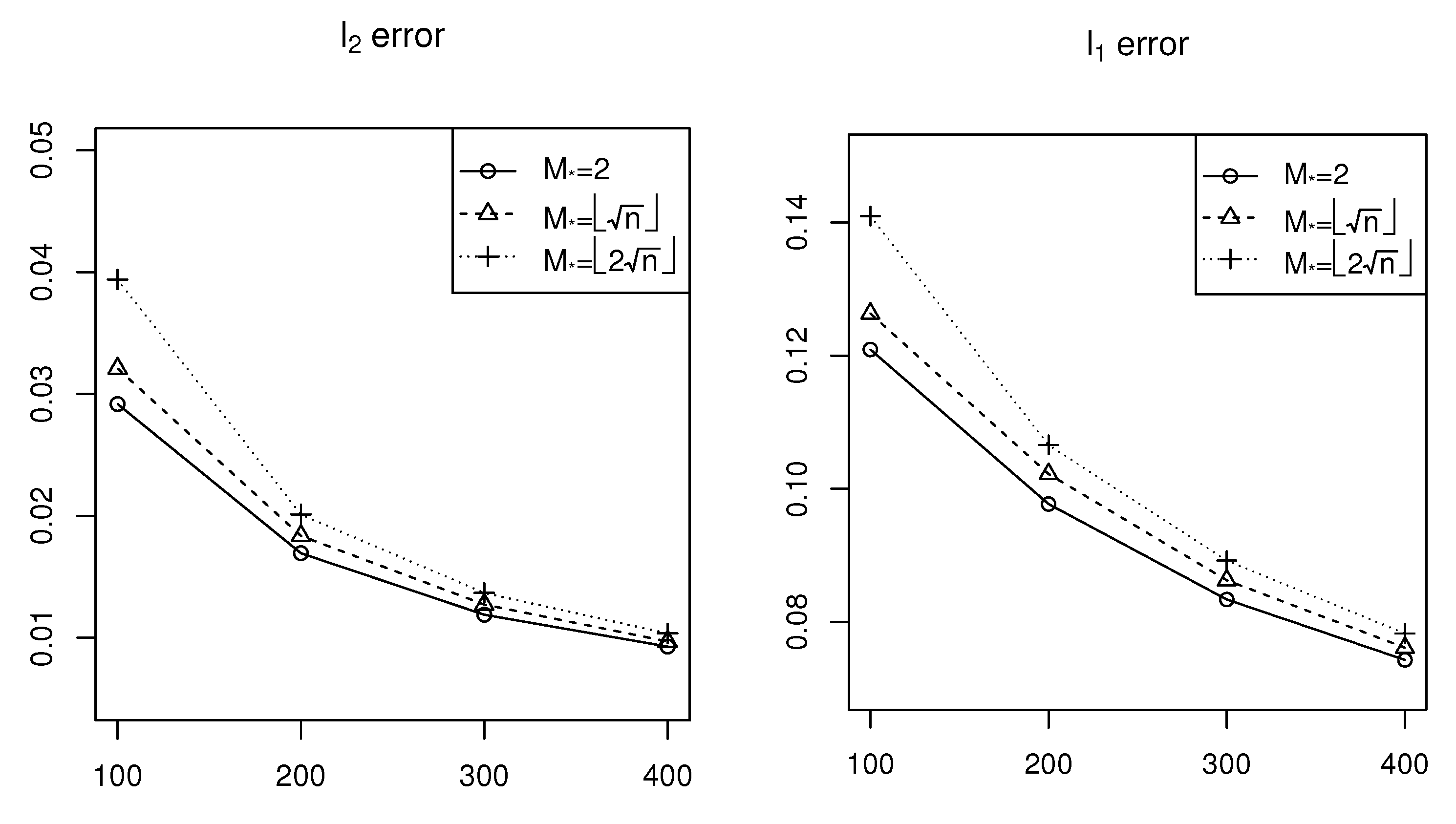
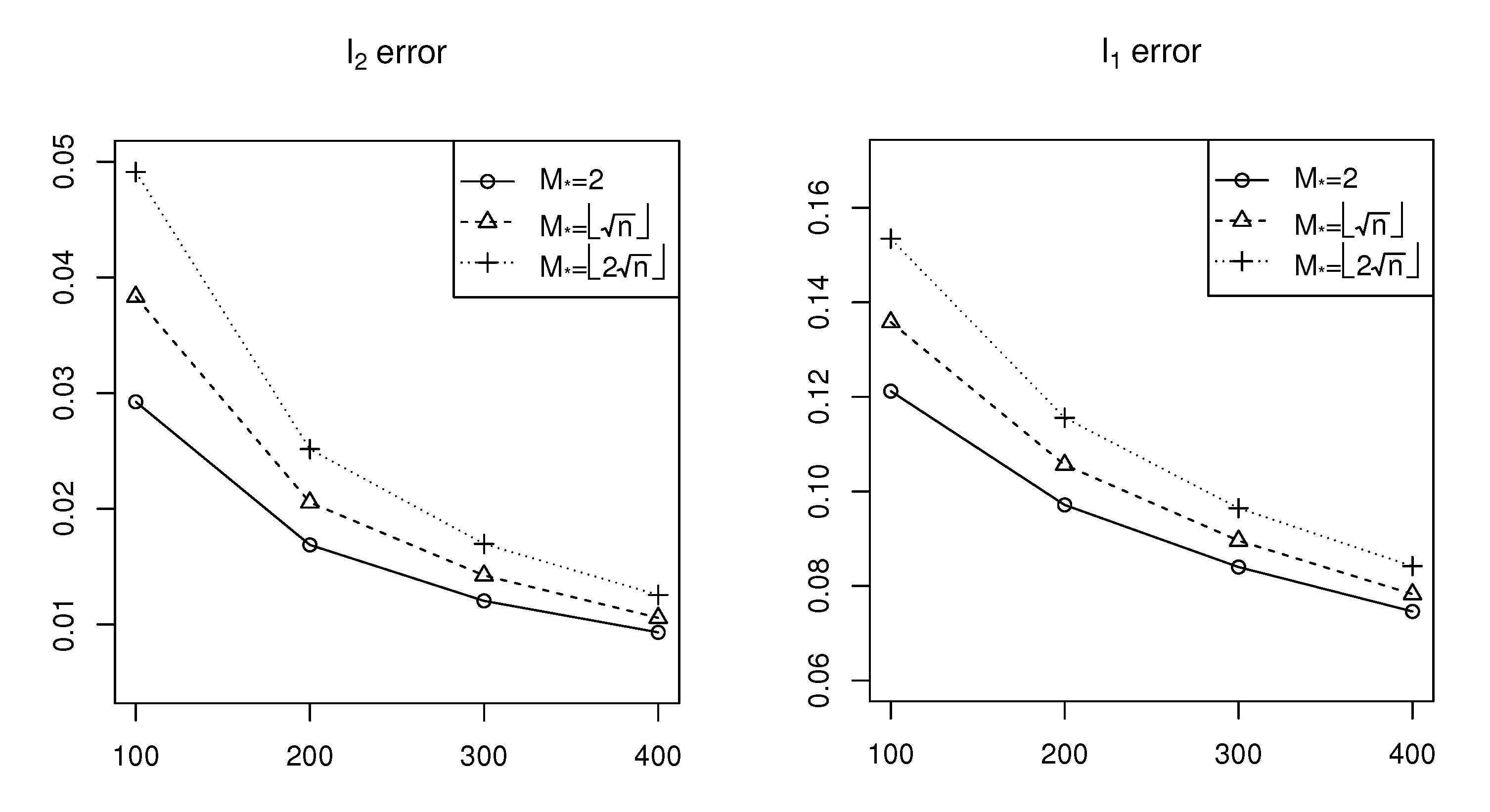
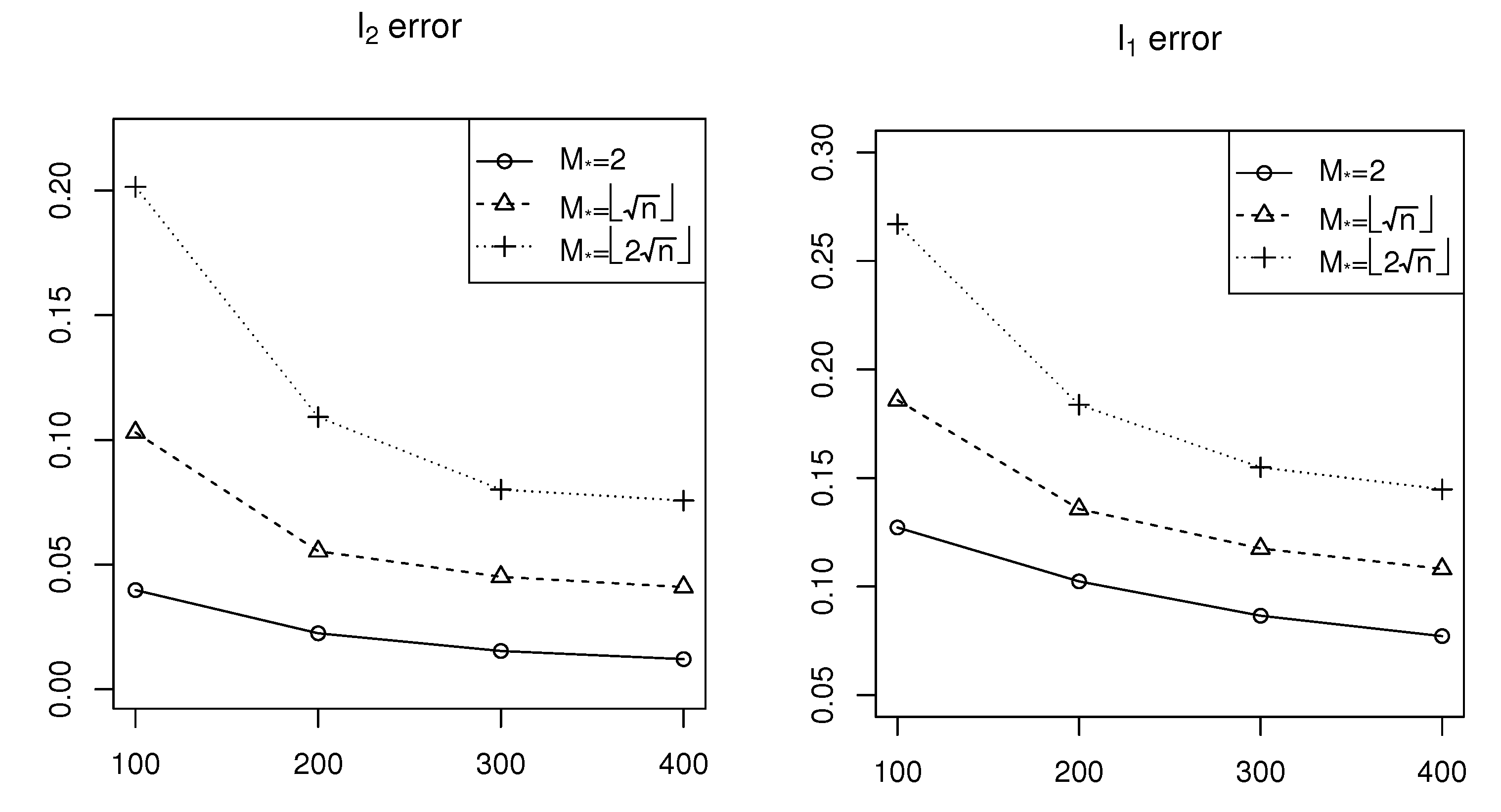
The simulation results are shown in Figure 1, Figure 2 and Figure 3 for Cases 1–3, respectively. According to Figure 1, we can see that both the ${𝓁}_2$ error and the ${𝓁}_1$ error decrease as the network size (n) increases, which means the estimation accuracy of $\widehat{\mathit{\beta }}$ generally improves as n increases. On the other hand, both the ${𝓁}_2$ error and the ${𝓁}_1$ error increase as $\mid M\left({\beta }^{*}\right)\mid$ increases, corresponding to variation in the sparsity level from sparse to dense, that is, the estimation accuracy of $\widehat{\mathit{\beta }}$ improves for sparse cases. Similar conclusions can be obtained from Figure 2 and Figure 3 relative to that derived from Figure 1.

Figure 1. Simulation results of ${𝓁}_2$ error and ${𝓁}_1$ error for Case 1.

Figure 2. Simulation results of ${𝓁}_2$ error and ${𝓁}_1$ error for Case 2.

Figure 3. Simulation results of ${𝓁}_2$ error and ${𝓁}_1$ error for Case 3.

Comparing Figure 1, Figure 2 and Figure 3 vertically, it is observable that as the signal strength or signal-to-noise ratio of ${\mathit{\beta }}^{*}$ increases, estimation errors also increase. This indicates an inverse relationship between the estimation accuracy and the signal-to-noise ratio. These simulation results show the efficiency of the estimation procedure of the sparse $\beta$ model with ${𝓁}_1$ penalty proposed in this paper.

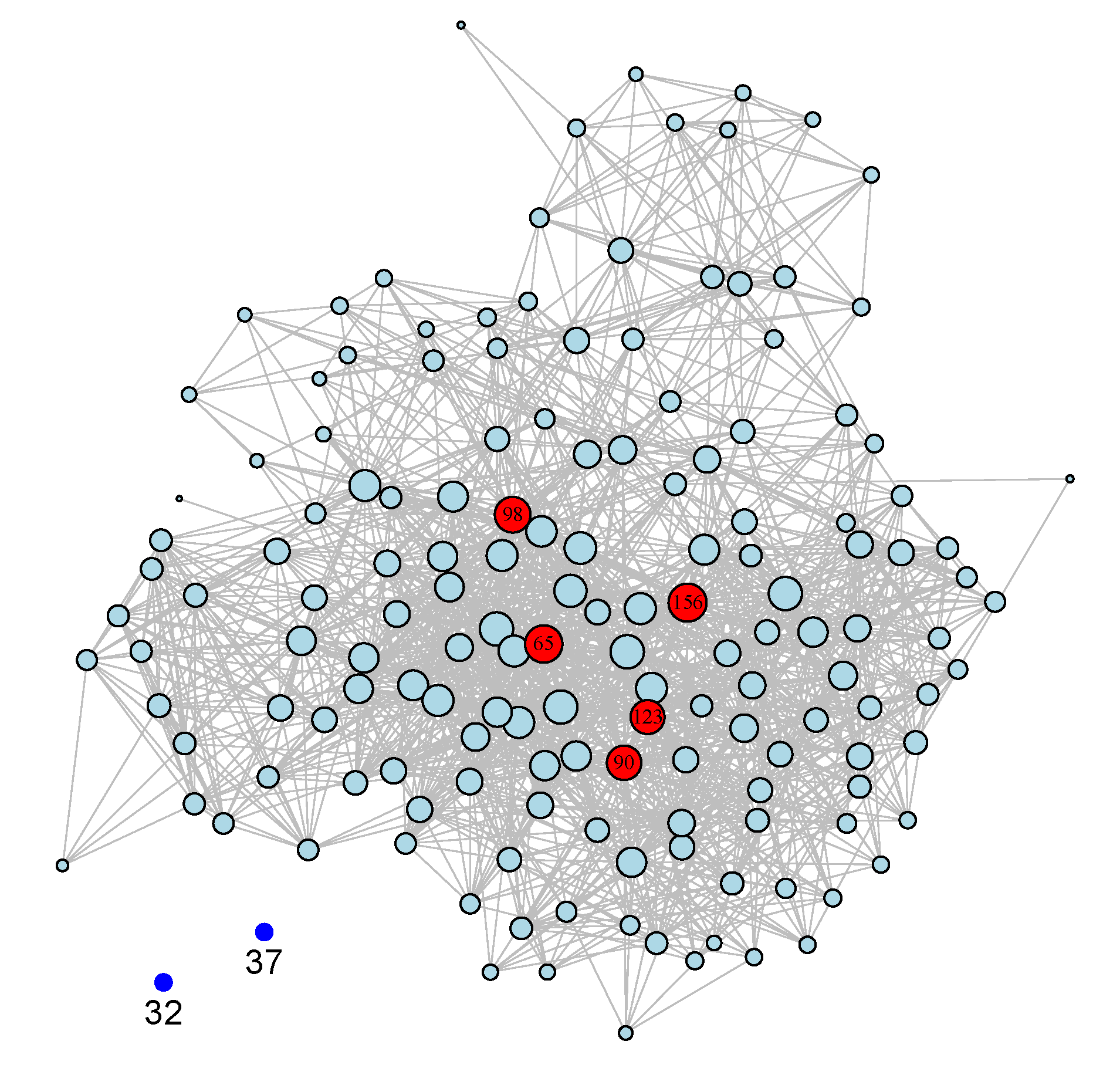
Finally, we use an example to introduce an undirected graph. We use the Enron email dataset as an example analysis [26] available from (https://www.cs.cmu.edu/~enron/, accessed on 7 May 2015). This dataset was originally acquired and made public by the Federal Energy Regulatory Commission during its investigation into fraudulent accounting practices. Some of the emails were deleted upon requests from affected employees. Therefore, the raw data are messy and need to be cleaned before any analysis is conducted. Ref. [27] applied data cleaning strategies to compile the Enron email dataset. We use their cleaned data for the subsequent analysis. We treat the data as a simple, undirected graph for our analysis, where each edge denotes that there is at least one message between the corresponding two nodes. For our analysis, we exclude messages with more than ten recipients, which is a subjectively chosen cutoff. The dataset contains 156 nodes with 1634 undirected edges, as shown in Figure 4. The quantiles of $0,1/4,1/2,3/4$, and 1 are 0, 13, 19, 27, and 55 for the degrees, respectively. The sparse $\beta$ model can capture node heterogeneity. For example, the degree of the 52th node is 1, and the degree of the 156th node is 55. It is therefore natural to associate those important nodes with their individual parameters while leaving the less important nodes as background nodes without associated parameters.

Figure 4. Enron email dataset. The vertex sizes are proportional to nodal degrees. The red circles indicate a nodal degree of more than 43. The blue circles indicate isolated nodes.

5. Conclusions

In this study, we investigated a sparse $\beta$ model with an ${𝓁}_1$ penalty in the dynamic field of network data models. The degree parameter was estimated through an ${𝓁}_1$ regularization problem, which can be easily solved by the proximal gradient descent method due to the convexity of the loss function. We established an optimal bound, corroborating the consistency of our proposed estimator, with empirical validations underscored by comprehensive simulation studies. One pivotal avenue for future research emanates from the unearthing and integration of alternative penalties that are more adaptive and efficient, facilitating enhanced model performance and a broader applicative scope. Furthermore, more effective optimization algorithms focusing on enhanced computational efficiency and adaptability to diverse network scenarios should be investigated in future studies. The sparse $\beta$ model proposed in this study serves as both a theoretical foundation and an algorithmic reference for future explorations into the sparse structures of other network models, such as network models with covariates [28], as well as functional covariates [29] partially functional covariates [30]. We aim to establish non-asymptotic optimal prediction error bounds. This contribution is instrumental in propelling the evolution of network models, offering insights and tools that can be adapted and optimized for diverse network structures and scenarios.

References

1. Fienberg, S.E. A brief history of statistical models for network analysis and open challenges. J. Comput. Graph. Stat. 2012, 21, 825–839. [Google Scholar] [CrossRef]
2. Erdös, P.; Rényi, A. On random graphs I. Publ. Math. Debr. 1959, 6, 18. [Google Scholar] [CrossRef]
3. Gilbert, E.N. Random graphs. Ann. Math. Stat. 1959, 30, 1141–1144. [Google Scholar] [CrossRef]
4. Kolaczyk, E.D.; Krivitsky, P.N. On the question of effective sample size in network modeling: An asymptotic inquiry. Stat. Sci. Rev. J. Inst. Math. Stat. 2015, 30, 184. [Google Scholar]
5. Newman, M. Networks; Oxford University Press: Oxford, UK, 2018. [Google Scholar]
6. Holland, P.W.; Laskey, K.B.; Leinhardt, S. Stochastic blockmodels: First steps. Soc. Netw. 1983, 5, 109–137. [Google Scholar] [CrossRef]
7. Chatterjee, S.; Diaconis, P.; Sly, A. Random graphs with a given degree sequence. Ann. Appl. Probab. 2011, 21, 1400–1435. [Google Scholar] [CrossRef]
8. Mukherjee, R.; Mukherjee, S.; Sen, S. Detection thresholds for the β-model on sparse graphs. Ann. Stat. 2018, 46, 1288–1317. [Google Scholar] [CrossRef]
9. Du, Y.; Qu, L.; Yan, T.; Zhang, Y. Time-varying β-model for dynamic directed networks. Scand. J. Stat. 2023. [Google Scholar] [CrossRef]
10. Abbe, E. Community Detection and Stochastic Block Models: Recent Developments. J. Mach. Learn. Res. 2018, 18, 6446–6531. [Google Scholar]
11. Rinaldo, A.; Petrović, S.; Fienberg, S.E. Maximum lilkelihood estimation in the β-model. Ann. Stat. 2013, 41, 1085–1110. [Google Scholar] [CrossRef]
12. Pan, L.; Yan, T. Asymptotics in the β-model for networks with a differentially private degree sequence. Commun. Stat. Theory Methods 2020, 49, 4378–4393. [Google Scholar] [CrossRef]
13. Luo, J.; Liu, T.; Wu, J.; Ahmed Ali, S.W. Asymptotic in undirected random graph models with a noisy degree sequence. Commun. Stat. Theory Methods 2022, 51, 789–810. [Google Scholar] [CrossRef]
14. Fan, Y.; Zhang, H.; Yan, T. Asymptotic Theory for Differentially Private Generalized beta-models with Parameters Increasing. Stat. Interface 2020, 13, 385–398. [Google Scholar] [CrossRef]
15. Chen, N.; Olvera-Cravioto, M. Directed random graphs with given degree distributions. Stoch. Syst. 2013, 3, 147–186. [Google Scholar] [CrossRef]
16. Kim, H.; Del Genio, C.I.; Bassler, K.E.; Toroczkai, Z. Constructing and sampling directed graphs with given degree sequences. New J. Phys. 2012, 14, 023012. [Google Scholar] [CrossRef]
17. Yan, T.; Leng, C.; Zhu, J. Asymptotics in directed exponential random graph models with an increasing bi-degree sequence. Ann. Stat. 2016, 44, 31–57. [Google Scholar] [CrossRef]
18. Yan, T.; Xu, J. A central limit theorem in the β-model for undirected random graphs with a diverging number of vertices. Biometrika 2013, 100, 519–524. [Google Scholar] [CrossRef]
19. Chen, M.; Kato, K.; Leng, C. Analysis of networks via the sparse β-model. J. R. Stat. Soc. Ser. B Stat. Methodol. 2021, 83, 887–910. [Google Scholar] [CrossRef]
20. Karwa, V.; Slavković, A. Inference Using Noisy Degrees: Differentially Private Beta-Model and Synthetic Graphs. Ann. Stat. 2016, 44, 87–112. [Google Scholar] [CrossRef]
21. Meinshausen, N.; Yu, B. Lasso-type recovery of sparse representations for high-dimensional data. Ann. Stat. 2009, 37, 246–270. [Google Scholar] [CrossRef]
22. Bickel, P.J.; Ritov, Y.; Tsybakov, A.B. Simultaneous analysis of Lasso and Dantzig selector. Ann. Stat. 2009, 37, 1705–1732. [Google Scholar] [CrossRef]
23. Huang, H.; Gao, Y.; Zhang, H.; Li, B. Weighted Lasso estimates for sparse logistic regression: Non-asymptotic properties with measurement errors. Acta Math. Sci. 2021, 41, 207–230. [Google Scholar] [CrossRef]
24. Bühlmann, P.; Van De Geer, S. Statistics for High-Dimensional Data: Methods, Theory and Applications; Springer Science & Business Media: Berlin/Heidelberg, Germany, 2011. [Google Scholar]
25. Zhang, H.; Chen, S.X. Concentration inequalities for statistical inference. Commun. Math. Res. 2021, 37, 1–85. [Google Scholar]
26. Cohen, W.W. Enron Email Dataset. Available online: https://www.cs.cmu.edu/enron/ (accessed on 7 May 2015).
27. Zhou, Y.; Goldberg, M.; Magdon-Ismail, M.; Wallace, A. Strategies for cleaning organizational emails with an application to enron email dataset. In Proceedings of the 5th Conference of North American Association for Computational Social and Organizational Science (No. 0621303), Atlanta, GA, USA, 7–9 June 2007. [Google Scholar]
28. Stein, S.; Leng, C. A Sparse β-Model with Covariates for Networks. arXiv 2020, arXiv:2010.13604. [Google Scholar]
29. Liu, C.; Zhang, H.; Jing, Y. Model-assisted estimators with auxiliary functional data. Commun. Math. Res. 2022, 38, 81–98. [Google Scholar] [CrossRef]
30. Zhang, H.; Lei, X. Growing-dimensional Partially Functional Linear Models: Non-asymptotic Optimal Prediction Error. Phys. Scr. 2023, 98, 095216. [Google Scholar] [CrossRef]