Abstract
The near-future parking space availability is informative for the formulation of parking-related policy in urban areas. Plenty of studies have contributed to the spatial–temporal prediction for parking occupancy by considering the adjacency between parking lots. However, their similarities in properties remain unspecific. For example, parking lots with similar functions, though not adjacent, usually have similar patterns of occupancy changes, which can help with the prediction as well. To fill the gap, this paper proposes a multi-view and attention-based approach for spatial–temporal parking occupancy prediction, namely hybrid graph convolution network with long short-term memory and temporal pattern attention (HGLT). In addition to the local view of adjacency, we construct a similarity matrix using the Pearson correlation coefficient between parking lots as the global view. Then, we design an integrated neural network focusing on graph structure and temporal pattern to assign proper weights to the different spatial features in both views. Comprehensive evaluations on a real-world dataset show that HGLT reduces prediction error by about 30.14% on average compared to other state-of-the-art models. Moreover, it is demonstrated that the global view is effective in predicting parking occupancy.
MSC:
68T09
1. Introduction
The huge number of vehicles in urban areas has posed many challenges not just to the dynamic transportation systems but also to the static ones. For example, an instance investigation [1] showed that only about 25% drivers did not cruise to find parking in the central business district of cities, which can result in unnecessary traffic congestion [2] and lead to additional emissions [3]. To reduce cruising time and optimize parking space utilization, various parking-related smart services have been developed, e.g., parking guidance, dynamic pricing, and space sharing [4,5]. As the foundation to enable these services, a spatial–temporal parking occupancy prediction method is required for regional parking occupancy prediction to provide the near-future parking occupancy in urban areas.
Spatio-temporal prediction is essential to further address parking challenges and optimize the operation of intra-city traffic flows compared to time series prediction, as today’s urban areas are well connected to each other. In this context, two challenges are emerging. First, the underlying features hidden in spatial–temporal data should be extracted to promote spatial–temporal parking occupancy prediction [6,7]. Moreover, considering that multivariate variables are introduced for spatial–temporal parking occupancy prediction, the flexible weighting of them is needed to achieve fair and reasonable predictions [8].
In the last decade, recurrent neural networks (RNNs) have dominated the time-series prediction in transportation research [9]. However, spatial dependencies are ignored in these methods. To fill the gap, plenty of related studies have recently proposed to utilize graph neural networks (GNNs) to embed adjacent relationships into time-series data, and achieve spatial–temporal prediction by combining GNNs with RNNs [10]. Such an integration has contributed to outstanding improvement in predictive accuracy. However, the fixed adjacent graph used in these methods has been always criticized due to the lack of a global view. We argue that parking lots with similar functions, though not adjacent, will generate similar demand changes, e.g., parking occupancy in different business districts would respond similarly to holidays [11]. Such a synchronization can be helpful for the spatial–temporal parking occupancy prediction. Moreover, even though many studies on traffic condition prediction have employed a novel technique, i.e., attention mechanism [12], for better parameter weighting in the past few years [13], an integration method is still lacking for the near-future spatial–temporal parking occupancy prediction via building an effective model with graph and temporal attentions.
To fill the research gap, we proposed a multi-view and attention-based approach for spatial–temporal parking occupancy prediction, namely hybrid graph convolution network with long short-term memory and temporal pattern attention (HGLT). The proposed approach HGLT consists of two modules: (1) The multi-view spatial module utilizes two separate graph attentional networks (GATs) [14] to extract the spatial features hidden in the adjacency and similarity matrices, respectively. The similarity between parking lots is measured by the Pearson correlation coefficient [15]. (2) The multivariate temporal module employs long short-term memory (LSTM) and temporal pattern attention (TPA) [13] to decode the multiple features given by the spatial module. A real-world dataset containing 35 parking lots in Guangzhou, China is used for model validation. The results empirically show that HGLT obtains the highest scores in all the six evaluation metrics, namely mean squared error (MSE) 0.0014, root mean square error (RMSE) 0.0353, mean absolute error (MAE) 0.0221, mean absolute percentage error (MAPE) 10.11%, relative absolute error (RAE) 15.47% and r-square () 86.04%. Compared to the state-of-the-art baselines, the proposed method reduces the prediction errors by 30.14% on average, and improves the degree of fit of the proposed method by 18.8% in on average in four prediction intervals. Moreover, the ablation experiment demonstrates the effectiveness of each component in the proposed model, and the global view can bring a 28.19% improvement in accuracy on average.
The main contributions of the study are as follows:
- In addition to the local view of adjacency, we consider the similarity in occupancy changes between parking lots in a global view to introduce more helpful information for prediction. The similarity between parking lots is determined by a typical metric for linear correlation, i.e., Pearson correlation coefficient.
- We design a hybrid graph convolution network to extract spatial features and integrate temporal pattern attention (TPA) to assign reasonable weights to different spatial features.
- The proposed approach HGLT is tested on a real-world dataset, and the results of the experiment empirically demonstrate that HGLT outperforms the representative models, and each component in the proposed method is effective.
2. Related Work
Regional parking occupancy prediction is one of the foundations of parking management and guidance systems, which can be considered a typical spatial–temporal prediction problem. Reliable and accurate regional parking occupancy prediction can recommend suitable parking spaces for drivers and help city managers dynamically adjust parking management strategies to improve the utilization of parking resources [16,17].
Previous studies on parking occupancy prediction fell into three main categories, i.e., statistical models, machine learning methods and deep neural networks. The statistical models make predictions by extracting the linear correlation of time series. For example, autoregressive integrated moving average (ARIMA) is utilized to predict the unoccupied parking space [18], which performs well when the change in remaining berth is relatively flat. However, the nonlinear correlation in the parking occupancy sequences remained unspecific in these studies, leading to poor prediction performance during sharp fluctuations [19]. Machine learning methods are widely used for parking lot occupancy prediction because they do not require linear assumptions. For example, a short-term prediction model for available parking space is proposed [20], which achieves a more accurate performance with a more efficient structure than the largest Lyapunov exponents (LEs) method. Combining the Support Vector Regression (SVR) and Fruit Fly Optimization Algorithm (FOA), a vacant parking space prediction method is proposed [21], which performs better than the back-propagation neural network (BPNN). A parking availability prediction model based on neural networks and random forests is proposed to demonstrate the role of WoT and AI in smart cities [22]. In recent years, computational and storage capabilities have been evolving, and deep learning has been widely used for intelligent traffic status prediction and parking occupancy prediction [23,24,25,26]. For example, a novel long short-term memory recurrent neural network (LSTM-NN) model is proposed to make multistep prediction for parking occupancy based on historical information [27]. A parking vacancy prediction model named DWT-Bi-LSTM was recently proposed, which combines wavelet transform (WT) and bi-directional long-short term memory (Bi-LSTM) [28] to decompose time series at multiple scales and extract bi-directional temporal features, respectively. However, the above studies only considered the temporal patterns and ignored the spatial correlation between parking lots.
Regional parking occupancy prediction needs to extract the spatial–temporal correlation. For example, an auto-regressive model [29] and a boosting method [30] for on-street parking availability prediction were proposed at an earlier time, which consider both temporal and spatial correlation. A neural network model for block-level parking lot occupancy prediction was proposed to extract spatial relationships of traffic flow using the convolutional neural network (CNN) and capture temporal correlation using stacked LSTM autoencoder [31], and the model outperformed multi-layer LSTM and Lasso. However, the non-Euclidean spatial correlation between parking lots is not taken into account by the CNN, and its prediction performance is limited. Since graph neural networks (GNNs) are good at processing non-Euclidean graph structure data [11,32,33], they have been widely used for spatial–temporal prediction in transportation research, such as traffic flow and speech [11,34,35,36]. Spatial–temporal parking occupancy prediction is not an exception. An illustration is the graph convolutional neural network and long short-term memory network (GCN-LSTM) [37], which uses graph convolutional neural networks to extract spatial relationships of traffic flows in large-scale networks and learns temporal features using long short-term memory (LSTM). For the purpose of further improvement in feature representation, attention mechanisms are introduced. Examples include hybrid spatial–temporal graph convolutional networks (HST-GCNs) [38] and semi-supervised hierarchical recurrent graph neural networks-X (SHARE-X) [39]. The HST-GCN introduces a focus mechanism based on the similarity of parking duration distributions to take into account long-term spatio-temporal correlations. SHARE-X employs a hierarchical graph attention module to learn the adjacencies between parking lots. A hierarchical recurrent network module was also constructed to incorporate short-term and long-term dynamic temporal dependencies of parking lots. Although these GNN-based methods contribute to introducing adjacent relationships between parking lots, features hidden in the parking lots with similar functions are omitted. Furthermore, an integrated model with graph attention and temporal pattern attention is still missing in spatial–temporal parking occupancy prediction.
In summary, previous spatial–temporal parking occupancy prediction methods mainly use GNNs to extract spatial correlation and RNNs to extract temporal correlation. These methods only consider the adjacency between parking lots but not the global correlation in spatial dependencies. And they do not consider the influence degree of different spatial dependencies on the prediction results. To fill these gaps, we propose a multi-view and attention-based model integrated by GAT, LSTM and TPA, which considers not just the adjacency between parking lots but also the similarity in parking occupancy changes.
3. Methodology
As shown in Figure 1, the proposed approach consists of a multi-view spatial module and multivariate temporal module. Specifically, the multi-view spatial module employs GAT to embed the graph data (i.e., the distance-based adjacency and correlation-based similarity) into dense vectors. The multivariate temporal module aligns LSTM and TPA to extract the underlying patterns hidden in the spatial–temporal features (i.e., the embedded vectors) given by the spatial module. Details of our method are discussed in the following subsections. There are three colors of squares in the model overview. Each colored square represents a feature of a viewpoint. The orange square indicates the matrix formed by the input raw data x. The blue squares indicate the matrices of the hidden layers of GAT S whose graph structure is generated based on distance. The green squares indicate the matrices of the hidden layers of GAT whose graph structure is generated based on similarity. The number of rows of these matrices is equal to the length of the sequence l. The number of columns of these matrices is equal to the number of parking lots. The feature matrices of different colors are stacked into a 3D tensor u and fed into a multivariate temporal module to achieve prediction after temporal feature extraction and attention allocation. In addition, the gray elements represent learnable model components. To ensure the seamless integration, the structure of each network component is shown in Table 1.
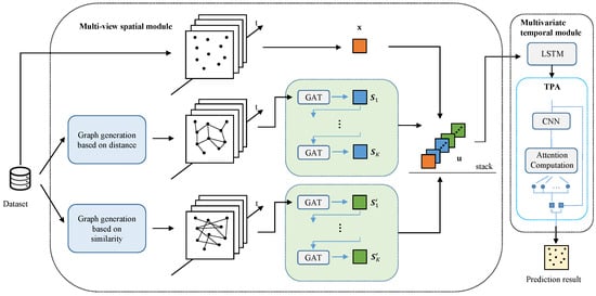
Figure 1.
Overview of the proposed model structure.

Table 1.
The list of network structure.
3.1. Problem Definition
In our work, parking occupancy is defined as the division of the number of in-used lots and the capacity of parking lots, ranging between 0 and 1. The objective of regional parking occupancy prediction is to use a unified model to simultaneously predict the near-future parking occupancy of multiple parking lots within a region based on the historical records of the specific region.
By considering parking lots as nodes and their relationships (such as distances and similarities) as edges, the objective function can be written as Equation (1), where represents the observed occupancy of all nodes at time t in a specific area, while represents the predicted ones at time ; l denotes the look-back window size, and denotes the predictive interval for the data-driven prediction model HGLT, respectively. Furthermore, given N parking lots in the studied area, , where is the value of occupancy in park i at time t, and the same for . The problem can be formulated as
where and denote the distance-based graph and similarity-based graph, respectively, which are described below.
3.2. Multi-View Spatial Module
We argue that parking-related spatial features can be categorized into two groups, i.e., distance-based adjacency and correlation-based similarity. From a local perspective, parking demand will propagate between neighboring parking lots, especially during peak hours. For example, when a park becomes crowded or its price is increased, drivers will be inclined to choose the neighboring parking lots as an alternative. Since such a propagation will decline as the distance increases, we determine the local spatial relationships between parking lots by their distances. On the other hand, from a global perspective, the features hidden in the parking lots with similar functions should be considered. For example, two commercial parking lots with the same type or points of interest will have similar patterns of change in parking occupancy. Moreover, parking lots for industrial areas will have high occupancy during work hours due to daily commuting, while the occupancy of parking lots for residential areas will be relatively low during this period. Therefore, we can also find a strong correlation between non-adjacent parking lots.
Therefore, to be comprehensive, the proposed method first constructs two graph structures based on distance and similarity, respectively. Then, two separate hierarchical graph attention mechanisms are employed to extract local and global spatial features from the two graphs, respectively.
3.2.1. Graph Convolution Based on Distance
We utilize the graph attentional network (GAT) [14] to simulate the demand propagation between parking lots. Specifically, by considering the traffic net as a graph, parks can be viewed as the nodes, while the connectivity of two parking lots can be viewed as the edges. In this work, the connectivity is determined by distance. Let be the graph based on distance. The connectivity of the i-th and j-th parking lot can be determined as follows:
where is the distance of the i-th and j-th parking lots in the road network, and D is the threshold value which can be set based on experience. represents the state of the connection between the the i-th and j-th parking lots. A value of 1 for means that the i-th and j-th parking lots are connected, while a value of 0 means that they are not connected.
The computing processes of GAT are divided into two steps. The input is a matrix , where is the input hidden state of the i-th node from moment to moment t, and N is the number of the nodes. The output of GAT is a matrix , where is the output hidden state of the i-th node from moment to moment t. Based on the , the attention score of the i-th and j-th nodes is expressed as Equation (3):
where is the parameter matrix of the fully connected network, and b is the bias of the fully connected network. “‖” means vector concat. LeakyReLU is a nonlinear activation function expressed as Equation (4):
where z represents the input variable.
Then, the hidden statuses are updated. For each node in the graph, the attention score of all its neighboring nodes is normalized using the softmax function. The calculation can be expressed as Equation (5):
where stands for the set of i-th node’s neighbors.
The output hidden state of the i-th node is calculated by the weighted average of neighboring nodes and the ReLU function, which is expressed as Equation (6):
Note that to prevent overfitting, dropout should be used in each layer of GAT (by default 0.2) as recommended in the original GAT paper [14]. Same below in Section 3.2.2.
Since a single layer of graph convolution can only consider the impact of neighboring parking lots, we use multi-layer graph convolution to model the impact of parking lots at different distances and output the results of each layer of graph convolution as features. Let the number of layers be K.
3.2.2. Graph Convolution Based on Similarity
The parking occupancy of a target parking lot may be synchronized with and show a similar or opposite parking occupancy change pattern to the parking occupancy of non-neighboring parking lots, which makes datasets of different parking lots strongly correlated. We adopt the Pearson correlation coefficient to model the synchronization between parking lots. If the Pearson correlation coefficient between two parking lots exceeds the threshold value, the two parking lots are considered connected. Then, we can construct a graph structure based on the Pearson correlation coefficient. The Pearson correlation coefficient is a statistical measure that quantifies the strength and direction of a linear relationship between two continuous variables. In other words, it measures how much one variable changes when the other variable changes in a linear fashion. Typically, when the coefficient < or >, the two variables are considered to be correlated at medium strength and above. The Pearson correlation coefficient between the i-th and j-th parking lots is calculated as follows:
where and are the parking occupancy of the i-th and j-th parking lots at time step t, and and are the average value of the parking occupancy of the i-th and j-th parking lots. n is the length of the time series.
Let be the graph based on similarity. The connectivity of the i-th and j-th parking lots can be determined as follows:
where is the Pearson correlation coefficient of the i-th and j-th parking lots in the road network, and C is the threshold value which can be set according to the actual needs. represents the state of the connection between the i-th and j-th parking lots. A value of 1 for means that the i-th and j-th parking lots are connected, while a value of 0 means that they are not connected.
The computing processes of GAT are divided into two steps. The input is a matrix , where is the input hidden state of the i-th node from moment to moment t, and N is the number of the nodes. The output of GAT is a matrix , where is the output hidden state of the i-th node from moment to moment t. Based on the , the attention score of the i-th and j-th nodes is expressed as Equation (9):
where is the parameter matrix of the fully connected network, and b is the bias of the fully connected network. LeakyReLU is a nonlinear activation function like Equation (4). “‖” means vector concat.
Then, the hidden statuses are updated. For each node in the graph, the attention score of all its neighboring nodes is normalized using the softmax function. The calculation can be expressed as Equation (10):
where stands for the set of the i-th node’s neighbors.
The output hidden state of the i-th node is calculated by the weighted average of neighboring nodes and the ReLU functions, which is expressed in Equation (11):
To model the impact of parking lots with different levels of synchronization, we use multi-layer graph convolution and output the results of each layer of graph convolution as the features. Let the number of layers be K.
Then, we stack the input vector and the output of each layer of the graph convolution modules as a feature matrix. The feature matrix can be expressed as follows:
where K is the the number of layers.
3.3. Multivariate Temporal Module
As shown in Figure 2, the proposed method adopts LSTM and TPA to detect the temporal pattern across multiple time steps in the feature series and assign weight to different features. First, the stacked feature tensor is fed to LSTM to exact the temporal feature. The hidden layer states of LSTM are divided into two parts. The hidden layer states from moment to moment t form the state matrix H, and the hidden layer state at the current moment t is used separately for scoring function computation and final prediction. Then k 1D CNN filters are separately used to convolve along the rows of the matrix to form a new feature matrix . Each colored box represents a convolution result of one filter in the feature matrix . Then, the scoring function calculates the attention weights for each row of the feature matrix . The feature vector is obtained by the weighted summation of the rows of the feature matrix and combined with the hidden layer state at the current moment t to make the final prediction.
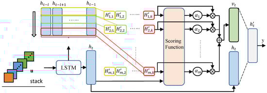
Figure 2.
The structure of multivariate temporal module.
3.3.1. Long Short-Term Memory
In order to extract the high-dimensional temporal patterns in parking occupancy, we adopt LSTM to build the temporal module. LSTM is a modified recurrent neural network (RNN) for processing and predicting significant events in time series with long intervals and delays [40].
LSTM generally defines a recurrent function and calculates for current time t, as Equation (13):
where is the hidden layer state of the LSTM at time t; m is the dimension of variables; is the final state of memory cell at time t; and is the value of feature sequence at time t.
The calculation is defined by Equation (14):
where t is the time step, is the input gate, is the forget gate, and is the output gate. , , and . , , , , , , and are the coefficient matrix. , , and , m, r are the dimension of the variable. , , and , and ⊙ denotes the element-wise multiplication.
3.3.2. Temporal Pattern Attention
Different spatial features are extracted in the spatial module. Different spatial features have different degrees of influence on the prediction results. Therefore, assigning different weights to different feature sequences can improve the prediction accuracy. A typical attention mechanism selects information from the previous time steps that is relevant to the current time step to help prediction but fails to capture temporal patterns across multiple time steps. And when there are multiple variables in each time step, the typical attention mechanism fails to select the variables relevant to the target time step. The temporal patterns attention (TPA) mechanism can assign weights to different variables to select those variables that are helpful for prediction. According to the state matrix of LSTM, the TPA first detects temporal patterns using CNN, then calculates the context vector with the attention mechanism and makes a prediction with the context vector at last.
As is shown in Figure 2, the state matrix consists of previous hidden layer states of LSTM, which is presented as Equation (15):
where t is the current moment, and l is the window size.
To detect the temporal pattern across multiple time steps in the feature series, the TPA module applies one-dimensional CNN filters on the row vectors of state matrix H. As is shown in Figure 2, there are k one-dimensional CNN filters with length l. The rectangles in different colors represent different filters. Each filter convolves over m features of state matrix and produces a matrix with m rows and k columns. represents the convolutional value of the i-th row vector and the j-th filter. The operation is given as Equation (16):
As is shown in Figure 2, according to the matrix , the scoring function calculates a weight for each row of by comparing it with the current hidden layer state . Then, the context vector is calculated by the weighted sum of the row vectors of . Then, the final prediction value is calculated with the context vector and the current hidden layer state .
The scoring function is defined as Equation (17).
where is the i-th row of , is the coefficient matrix, and .
The attention weight of the i-th row vector of , , is calculated as Equation (18):
Then, the row vectors of are weighted by to calculate the context vector :
Then, we integrate and to predict the target value:
where is the integrated vector; is the predictive value; , and are the coefficient matrix; and ; ; ; and .
4. Experiments and Results
In this section, the performance of the proposed method is tested with several representative parking occupancy prediction methods and traffic condition prediction methods through a real-world dataset.
4.1. Data Description
The dataset used in this paper consists of 35 parking lots in the central business district of Guangzhou, China as shown in Figure 3. All data are collected in real application scenarios. The types of parking lots are diverse (e.g., residential, commercial, hospital, and recreational). All parking lots have good property management and electronic access gates. Parking occupancy records of 1–30 June 2018 have a minimum resolution of five minutes. Therefore, from the temporal dimension, the data have a total of 8640 timestamps. Based on the driving distances, we construct an adjacency matrix of parking lots as shown in Figure 3. If the distance is less than 2 km, the two parks are considered connected with each other. In addition, we construct a similarity matrix based on the Pearson coefficients with a threshold of 0.4 between the studied parking lots as shown in Figure 4. By considering parking lots as nodes and their relationships as edges, two graphs are provided to the proposed model for spatial–temporal parking occupancy prediction.
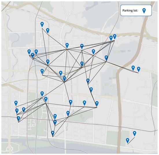
Figure 3.
Spatial distribution of the studied parking lots.
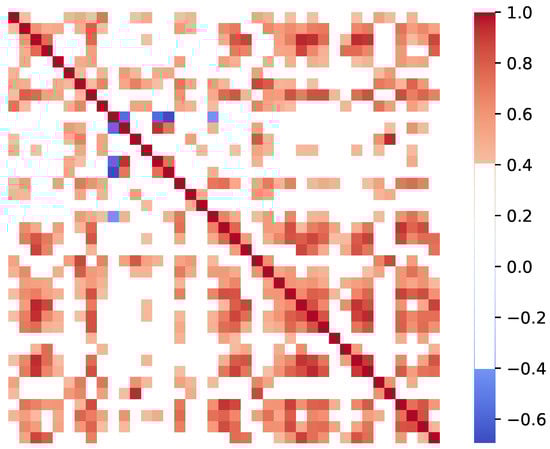
Figure 4.
Pearson correlation between different parking lots.
4.2. Evaluation Metrics
In order to make a comprehensive and fair comparison, six metrics, i.e., mean absolute percentage error (MAPE), mean absolute error (MAE), mean squared error (MSE), root mean squared error (RMSE), relative absolute error (RAE), and R-Square Coefficient () are used as the indicators of the performance of compared models. Their calculation formulas are presented in Equation (22):
where and are the observed and predicted values of sample i, respectively; is the mean value of samples; and M is the sample size.
4.3. Experimental Setup
Considering the huge success of neural networks (NNs) in spatial–temporal prediction, we select six representative NN-based models as competitive approaches. (1) The fully connected neural network (FCNN) is a network designed after the connectivity of biological neurons, which cannot distinguish between different types of features. (2) Long short-term memory (LSTM) [40] is an improved recurrent neural network with excellent temporal feature extraction capability. (3) The graph attention network (GAT) [14] is a neural network running on graph-structured data, which is able to assign different weights to different nodes in the neighborhood. (4) Du-parking [41] is a deep learning parking occupancy prediction model for Baidu Map, which is a business model that has been widely used in major cities, such as Shenzhen and Beijing. The model improves on the LSTM and consists of three main components that simulate the overall impact of the temporal data, the cycle and the current general influence. (5) GCNN + LSTM [37] is a spatial–temporal deep learning prediction model that uses graph convolutional neural networks (GCNNs) to extract the spatial relations and utilizes long-short term memory (LSTM) to capture the temporal features. (6) GATLSTM [42] is a model combining GAT and LSTM, which is able to assign reasonable weights on the graph and learn spatial–temporal features. For this, the typical prediction model LSTM is selected as the baseline.
The training and test sets are divided according to a ratio of 8 to 2 in every parking lot, which means the former 80% data can be used to train the model, and the remaining 20% can only be used for evaluation, which is a strict prohibition of information disclosure. We set the threshold of distance-based adjacency D to be 2 km, which is approximately 2 times to the 80th percentile of 1.35 km in walking trips investigated by [43]. It can be assumed that drivers will only look for parking in parking lots within a two-hop neighborhood of the target parking lot, due to the distance. So the number of the graph propagation K is set to 2. Then, the number of feature maps m is 5 (1 + 2 + 2). The five feature maps include local occupancy feature, 1-hop similarity-based neighbors feature, 2-hop similarity-based neighbors feature, 1-hop distance-based neighbors feature, and 2-hop distance-based neighbors feature. According to the example in the original TPA paper, the number of CNN filters is set equal to the feature dimension [13]. Therefore, the same setting is used for the experiments in this paper, i.e., . The threshold of Pearson-based similarity C is set to 0.4, leading to more than 60% of the edges’ as shown in Figure 4. Note that the hyperparameters should be set according to the actual application scenarios. Moreover, the test will be conducted to predict the parking occupancy rate in four time intervals, namely 15, 30, 45 and 60 min. Note that their prediction time steps are 3, 6, 9, and 12, respectively, as the temporal resolution of the dataset is 5 min. Since we use one previous hour’s data for prediction, the sequence length l is set to 12. And in all the learning methods, we use the uniform loss function MSE, which is widely used in regression tasks. Finally, some important running configurations of the proposed model and compared models are listed in Table 2. All the experiments are conducted on a Windows workstation with an NVIDIA Quadro RTX 4000 GPU, an Intel(R) Core(TM) i9-10900K CPU, and 64G RAM. To ensure that the model is reproducible, we share our code on a Github link (https://github.com/kuanghx3/HGLT, acessed on 15 September 2023).
Table 2.
List of running configurations.
4.4. Experiment Results and Discussion
The performance of the evaluated methods is analyzed in three parts, namely (1) the comparison experiment, to illustrate the good performance of the proposed model; (2) the ablation experiment, to verify each module’s effectiveness for prediction accuracy improvement; and (3) the feature importance, to demonstrate that the weight assignment of the proposed model is effective and reliable.
4.4.1. Comparison Experiment
As shown in Table 3, the evaluation metrics of the compared models are summarized. The results empirically show that the RNN model (i.e., LSTM) outperforms the GNN one (i.e., GAT) in all the metrics, while GAT is even inferior to the model with the simplest neural network, i.e., FCNN, indicating that GNNs alone are ineffective for the spatial–temporal prediction. Moreover, we can see that LSTM outperforms the integration of GCNN and LSTM, but is inferior to that of GAT and LSTM, suggesting that the graph attentions can bring better improvement in feature extraction than the typical graph convolution behavior. In contrast, the proposed method HGLT reduces the prediction error significantly with the highest scores in all six evaluation metrics, namely MSE 0.0014, RMSE 0.0353, MAE 0.0221, MAPE 10.11%, RAE 15.47% and 86.04%. Compared to other methods, the proposed method reduces the prediction errors by 30.14% on average, especially with a 38.15% reduction in MSE, a 21.12% reduction in RMSE, a 23.81% reduction in MAE, a 43.78% reduction in MAPE, and a 23.81% reduction in RAE, and improves the degree of fit of the proposed method by 18.8% in on average in four prediction intervals. Furthermore, the proposed method HGLT on average reduces the prediction error over the baseline model LSTM by 17.42% in MSE, 10.22% in RMSE, 8.43% in MAE, 17.02% in MAPE, and 8.43% in RAE, and improves the degree of fit of the proposed method by 1.94% in . And compared to GATLSTM, the proposed method HGLT on average reduces the prediction error by 8.93% in MSE, 5.05% in RMSE, 3.64% in MAE, 9.76% in MAPE, and 3.64% in RAE, and improves the degree of fit of the proposed method by 1.26% in . The comparisons illustrate that the spatial and temporal modules can work jointly and smoothly to achieve the best performance.
Table 3.
The list of evaluation metrics of compared models in different intervals.
To evaluate the learning capability of compared models, a line plot is drawn to illustrate their convergence profile in the training process. As shown in Figure 5, a best convergence profile is obtained by the proposed model. The black line see a loss drop at around 130 epochs, while other models require more than 250 epochs. Moreover, in the 800th epoch, the loss of the model in this paper is decreased closely to , while the loss of other models except GATLSTM is still around , where e is the natural logarithm. In addition, the outstanding performance obtained by GATLSTM indicates again that the graph attention is effective for the spatial–temporal parking occupancy prediction.
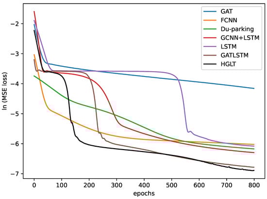
Figure 5.
Convergence profile of the compared models.
4.4.2. Ablation Experiment
In order to verify the effectiveness of each component in our model, i.e., the graph attentions on adjacency and similarity, the temporal modules with LSTM and TPA, we conduct an ablation experiment with all the parking lots in all the four prediction intervals. The results are illustrated in Table 4. The usefulness of a module can be demonstrated by the decrease in accuracy, i.e., the more the accuracy decreases after removing it, the more useful the module is. From the table, the proposed model has a 43.45% improvement over the model without LSTM on average, a 28.80% improvement over the model without adjacency, a 28.19% improvement over the model without similarity, and a 9.85% improvement over the model without TPA. It can be concluded that LSTM plays the most significant role in spatial–temporal parking occupancy prediction. More importantly, although the adjacent graph relationship ranks second, the graph convolution based on similarity between parking lots provides 28.19% improvement in accuracy on average, ranking third. Even though TPA delivers the smallest boost, it also results in a 9.85% improvement compared to the full model. The ablation experiment proves the effectiveness of each component in the proposed model.
Table 4.
The list of evaluation metrics of ablation experiments.
4.4.3. Feature Importance
In this subsection, the temporal and spatial attentions are visualized to demonstrate the reliability of the attention assignment of the proposed model. First, through adding a normal distribution noise to each time steps of the input features, the temporal feature importance is estimated according to the corresponding responses as shown in Figure 6. The figure shows that the occupancy data closest to the current moment (i.e., t and ) are most heavily weighted in the prediction, while the attentions allocated at all other times are numerically similar, which is in line with common sense. In terms of the spatial features, we derive the network weights assigned to the five feature maps of the observed local occupancy, 1-hop similarity-based neighbors, 2-hop similarity-based neighbors, 1-hop distance-based neighbors, and 2-hop similarity-based neighbors. As shown in Figure 7, attention on the 1-hop distance-based feature map is greater than that on the 2-hop one, consistent with the assumption that changes in needs brought about by first-order neighbors are more pronounced. In contrast, attention on the 1-hop similarity-based feature map is less than that on the 2-hop one, indicating that a less similar park can also provide helpful information to the target parks. In overall, it can be concluded that the adjacency and similarity between parking lots are both significant for spatial–temporal parking occupancy prediction.
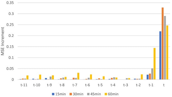
Figure 6.
The importance of the input features at different moment in prediction.
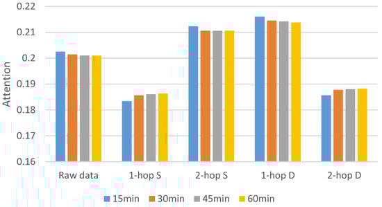
Figure 7.
Attention of the five feature maps, where S and D denote the similarity- and distance-based features, respectively.
5. Conclusions and Future Work
Spatial–temporal parking occupancy prediction is a essential technology of Parking Guidance and Information (PGI) systems. The accurate and effective regional parking occupancy prediction can improve the parking efficiency and utilization of parking resources, alleviate parking problems and reduce traffic congestion and pollution. Previous studies on spatial–temporal parking occupancy prediction have always considered the correlation of adjacent parking lots and ignored the correlation between un-adjacent parking lots. The parking lots with similar functions, though not adjacent, will generate similar demand changes, e.g., parking occupancy in different business districts would respond similarly to holidays [11]. Considering that the attention mechanism can improve the parameter weights of the model, we propose a multi-view graph neural network with spatial and temporal attention. In addition to the local adjacency, we consider the global similarity between parking lots. Specifically, the proposed model consists of two modules, i.e., multi-view spatial module and multivariate temporal module, for multi-view graph feature embedding and multivariate temporal decoding, respectively.
Through a comprehensive evaluation on a real-world dataset with 35 parking lots, the global view (i.e., the similarity matrix calculated by Pearson correlation coefficient) and the integration of GAT, LSTM and TPA enable the highly accurate spatial–temporal prediction. As shown by the evaluation results, the proposed approach outperforms other state-of-the-art models in three aspects, namely (1) the prediction errors can significantly reduce the prediction error by 30.14% on average in five regression metrics, i.e., MSE, RMSE, MAE, MAPE, and RAE in four prediction intervals; (2) the proposed model achieves optimal convergence, which sees the loss drop faster than in other models; and (3) HGLT assigns attention on different spatial features reasonably, indicating the effectiveness of its attention-based integration.
Although providing promising results, the model needs to be improved in the future work within the three directions: (1) Introduce multi-source data and consider the dynamic changes: Traffic status is affected by a variety of other factors, including weather, public emergencies, etc. This introduces perturbation to the time-series data and makes prediction difficult. It is worthwhile to explore methodologies for introducing multi-source data and enhancing the model’s adaptability to such changes. (2) Apply to more scenarios: Different scenarios may have different transportation patterns, so it is necessary to investigate the applicability of the model in different urban environments. (3) Apply the model to a parking guidance system: Parking guidance systems are downstream applications of parking occupancy prediction, informing drivers about parking space availability. This enables engineering applications and artificial intelligence to be effectively combined to improve the practical capability of the model.
Author Contributions
Conceptualization, W.Y.; Methodology, W.Y. and H.K.; software, W.Y. and H.K.; Validation, W.Y.; Formal analysis, W.Y., X.L. and J.L.; Investigation, W.Y.; Resources, J.L.; Data curation, W.Y.; Writing—original draft, W.Y.; Writing—review and editing, W.Y., H.K., X.L. and J.L.; Visualization, W.Y. and H.K.; Supervision, J.L.; Project administration, J.L.; Funding acquisition, J.L. All authors have read and agreed to the published version of the manuscript.
Funding
This research was funded by Guangdong Key Areas R&D Program grant number No. 2019B090913001.
Data Availability Statement
The dataset and origin code can be obtained on a Github link (https://github.com/kuanghx3/HGLT, acessed on 15 September 2023).
Conflicts of Interest
The authors declare no conflict of interest.
References
- Assemi, B.; Baker, D.; Paz, A. Searching for on-street parking: An empirical investigation of the factors influencing cruise time. Transp. Policy 2020, 97, 186–196. [Google Scholar] [CrossRef]
- Luleseged, T.S.; Di, M. Cooperative Multiagent System for Parking Availability Prediction Based on Time Varying Dynamic Markov Chains. J. Adv. Transp. 2017, 2017, 1760842. [Google Scholar]
- Bock, F.; Di Martino, S.; Origlia, A. Smart Parking: Using a Crowd of Taxis to Sense On-Street Parking Space Availability. IEEE Trans. Intell. Transp. Syst. 2020, 21, 496–508. [Google Scholar] [CrossRef]
- Qian, Z.S.; Rajagopal, R. Optimal dynamic parking pricing for morning commute considering expected cruising time. Transp. Res. Part C Emerg. Technol. 2014, 48, 468–490. [Google Scholar] [CrossRef]
- You, L.; Danaf, M.; Zhao, F.; Guan, J.; Azevedo, C.L.; Atasoy, B.; Ben-Akiva, M. A Federated Platform Enabling a Systematic Collaboration Among Devices, Data and Functions for Smart Mobility. IEEE Trans. Intell. Transp. Syst. 2023, 24, 4060–4074. [Google Scholar] [CrossRef]
- Wang, P.; Fu, Y.; Liu, G.; Hu, W.; Aggarwal, C. Human Mobility Synchronization and Trip Purpose Detection with Mixture of Hawkes Processes. In Proceedings of the 23rd ACM Sigkdd International Conference on Knowledge Discovery and Data Mining, Halifax, NS, USA, 13–17 August 2017; Association for Computing Machinery: New York, NY, USA, 2017; pp. 495–503. [Google Scholar] [CrossRef]
- Liu, Y.; Liu, C.; Lu, X.; Teng, M.; Zhu, H.; Xiong, H. Point-of-Interest Demand Modeling with Human Mobility Patterns. In Proceedings of the KDD’17: Proceedings of the 23rd Acm Sigkdd International Conference on Knowledge Discovery and Data Mining, Halifax, NS, USA, 13–17 August 2017; Assoc Comp Machinery SIGKDD: New York, NY, USA, 2017; pp. 947–955. [Google Scholar] [CrossRef]
- Ma, R.; Chen, S.; Zhang, H.M. Time series relations between parking garage occupancy and traffic speed in macroscopic downtown areas—A data driven study. J. Intell. Transp. Syst. 2021, 25, 423–438. [Google Scholar] [CrossRef]
- Khan, Z.; Khan, S.M.; Dey, K.; Chowdhury, M. Development and Evaluation of Recurrent Neural Network-Based Models for Hourly Traffic Volume and Annual Average Daily Traffic Prediction. Transp. Res. Record 2019, 2673, 489–503. [Google Scholar] [CrossRef]
- Zhu, H.; Xie, Y.; He, W.; Sun, C.; Zhu, K.; Zhou, G.; Ma, N. A Novel Traffic Flow Forecasting Method Based on RNN-GCN and BRB. J. Adv. Transp. 2020, 2020, 7586154. [Google Scholar] [CrossRef]
- Zhang, D.; Li, J. Multi-View Fusion Neural Network for Traffic Demand Prediction. Inf. Sci. 2023, 646, 119303. [Google Scholar] [CrossRef]
- Hu, H.; Lin, Z.; Hu, Q.; Zhang, Y. Attention Mechanism With Spatial-Temporal Joint Model for Traffic Flow Speed Prediction. IEEE Trans. Intell. Transp. Syst. 2022, 23, 16612–16621. [Google Scholar] [CrossRef]
- Shih, S.Y.; Sun, F.K.; Lee, H.Y. Temporal pattern attention for multivariate time series forecasting. Mach. Learn. 2019, 108, 1421–1441. [Google Scholar] [CrossRef]
- Veličković, P.; Cucurull, G.; Casanova, A.; Romero, A.; Liò, P.; Bengio, Y. Graph Attention Networks. arXiv 2017, arXiv:1710.10903. [Google Scholar]
- Feng, W.; Zhu, Q.; Zhuang, J.; Yu, S. An expert recommendation algorithm based on Pearson correlation coefficient and FP-growth. Clust. Comput. J. Netw. Softw. Tools Appl. 2019, 22, S7401–S7412. [Google Scholar] [CrossRef]
- Balmer, M.; Weibel, R.; Huang, H. Value of incorporating geospatial information into the prediction of on-street parking occupancy—A case study. Geo-Spat. Inf. Sci. 2021, 24, 438–457. [Google Scholar] [CrossRef]
- Tamrazian, A.; Qian, Z.; Rajagopal, R. Where is my parking spot? Online and offline prediction of time-varying parking occupancy. Transp. Res. Rec. 2015, 2489, 77–85. [Google Scholar] [CrossRef]
- Yu, F.; Guo, J.; Zhu, X.; Shi, G. Real Time Prediction of Unoccupied Parking Space Using Time Series Model. In Proceedings of the 3rd International Conference on Transportation Information and Safety (ICTIS 2015), Wuhan, China, 25–28 June 2015; Yan, X., Hu, Z., Zhong, M., Wu, C., Yang, Z., Eds.; Wuhan University Technol; China Commun Transportat Assoc; ASCE; Canadian Soc Civil Engn. IEEE: Piscataway, NJ, USA, 2015; pp. 370–374. [Google Scholar]
- Xiao, X.; Peng, Z.; Lin, Y.; Jin, Z.; Shao, W.; Chen, R.; Cheng, N.; Mao, G. Parking Prediction in Smart Cities: A Survey. IEEE Trans. Intell. Transp. Syst. 2023, 24, 10302–10326. [Google Scholar] [CrossRef]
- Ji, Y.; Tang, D.; Blythe, P.; Guo, W.; Wang, W. Short-term forecasting of available parking space using wavelet neural network model. IET Intell. Transp. Syst. 2015, 9, 202–209. [Google Scholar] [CrossRef]
- Fan, J.; Hu, Q.; Tang, Z. Predicting vacant parking space availability: An SVR method with fruit fly optimisation. IET Intell. Transp. Syst. 2018, 12, 1414–1420. [Google Scholar] [CrossRef]
- Provoost, J.C.; Kamilaris, A.; Wismans, L.J.J.; Van der Drift, S.; Van Keulen, M. Predicting parking occupancy via machine learning in the web of things. Internet Things 2020, 12, 100301. [Google Scholar] [CrossRef]
- Li, J.; Qu, H.; You, L. An Integrated Approach for the Near Real-Time Parking Occupancy Prediction. IEEE Trans. Intell. Transp. Syst. 2023, 24, 3769–3778. [Google Scholar] [CrossRef]
- Qu, H.; Liu, S.; Li, J.; Zhou, Y.; Liu, R. Adaptation and Learning to Learn (ALL): An Integrated Approach for Small-Sample Parking Occupancy Prediction. Mathematics 2022, 10, 2039. [Google Scholar] [CrossRef]
- Su, H.; Mo, S.; Peng, S.; Farhi, N. Short-Term Prediction of Time-Varying Passenger Flow for Intercity High-Speed Railways: A Neural Network Model Based on Multi-Source Data. Mathematics 2023, 11, 3446. [Google Scholar] [CrossRef]
- You, L.; Liu, S.; Chang, Y.; Yuen, C. A Triple-Step Asynchronous Federated Learning Mechanism for Client Activation, Interaction Optimization, and Aggregation Enhancement. IEEE Internet Things J. 2022, 9, 24199–24211. [Google Scholar] [CrossRef]
- Fan, J.; Hu, Q.; Xu, Y.; Tang, Z. Predicting vacant parking space availability: A long short-term memory approach. IEEE Intell. Trans. Syst. Mag. 2020, 14, 129–143. [Google Scholar] [CrossRef]
- Zeng, C.; Ma, C.X.; Wang, K.; Cui, Z.H. Predicting vacant parking space availability: A DWT-Bi-LSTM model. Phys. A Stat. Mech. Appl. 2022, 599, 127498. [Google Scholar] [CrossRef]
- Rajabioun, T.; Ioannou, P.A. On-Street and Off-Street Parking Availability Prediction Using Multivariate Spatiotemporal Models. IEEE Trans. Intell. Transp. Syst. 2015, 16, 2913–2924. [Google Scholar] [CrossRef]
- Fusek, R.; Mozdren, K.; Surkala, M.; Sojka, E. AdaBoost for Parking Lot Occupation Detection. In Proceedings of the 8th International Conference On Computer Recognition Systems Cores 2013, Wroclaw, Poland, 25–27 May 2013; Burduk, R., Jackowski, K., Kurzynski, M., Wozniak, M., Zolnierek, A., Eds.; CH-6330: Cham, Switzerland, 2013; Volume 226, pp. 681–690. [Google Scholar] [CrossRef]
- Ghosal, S.; Bani, A.; Amrouss, A.; El Hallaoui, I. A Deep Learning Approach to Predict Parking Occupancy using Cluster Augmented Learning Method. In Proceedings of the 2019 International Conference on Data Mining Workshops (ICDMW), Beijing, China, 8–11 November 2019; Papapetrou, P., Cheng, X., He, Q., Eds.; IEEE: Piscataway, NJ, USA, 2019; pp. 581–586. [Google Scholar]
- Wu, Z.; Pan, S.; Chen, F.; Long, G.; Zhang, C.; Yu, P.S. A Comprehensive Survey on Graph Neural Networks. IEEE Trans. Neural Netw. Learn. Syst. 2021, 32, 4–24. [Google Scholar] [CrossRef]
- Zhang, Z.; Cui, P.; Zhu, W. Deep Learning on Graphs: A Survey. IEEE Trans. Knowl. Data Eng. 2022, 34, 249–270. [Google Scholar] [CrossRef]
- Tang, C.; Sun, J.; Sun, Y.; Peng, M.; Gan, N. A General Traffic Flow Prediction Approach Based on Spatial-Temporal Graph Attention. IEEE Access 2020, 8, 153731–153741. [Google Scholar] [CrossRef]
- Cui, Z.; Henrickson, K.; Ke, R.; Wang, Y. Traffic Graph Convolutional Recurrent Neural Network: A Deep Learning Framework for Network-Scale Traffic Learning and Forecasting. IEEE Trans. Intell. Transp. Syst. 2020, 21, 4883–4894. [Google Scholar] [CrossRef]
- Liang, M.; Liu, R.W.; Zhan, Y.; Li, H.; Zhu, F.; Wang, F.Y. Fine-Grained Vessel Traffic Flow Prediction With a Spatio-Temporal Multigraph Convolutional Network. IEEE Trans. Intell. Transp. Syst. 2022, 23, 23694–23707. [Google Scholar] [CrossRef]
- Yang, S.; Ma, W.; Pi, X.; Qian, S. A deep learning approach to real-time parking occupancy prediction in transportation networks incorporating multiple spatio-temporal data sources. Transp. Res. Part C-Emerg. Technol. 2019, 107, 248–265. [Google Scholar] [CrossRef]
- Xiao, X.; Jin, Z.; Hui, Y.; Xu, Y.; Shao, W. Hybrid Spatial-Temporal Graph Convolutional Networks for On-Street Parking Availability Prediction. Remote Sens. 2021, 13, 3338. [Google Scholar] [CrossRef]
- Zhang, W.; Liu, H.; Liu, Y.; Zhou, J.; Xu, T.; Xiong, H. Semi-Supervised City-Wide Parking Availability Prediction via Hierarchical Recurrent Graph Neural Network. IEEE Trans. Knowl. Data Eng. 2022, 34, 3984–3996. [Google Scholar] [CrossRef]
- Hochreiter, S.; Schmidhuber, J. Long Short-Term Memory. Neural Comput. 1997, 9, 1735–1780. [Google Scholar] [CrossRef]
- Rong, Y.; Xu, Z.; Yan, R.; Xu, M. Du-Parking: Spatio-Temporal Big Data Tells You Realtime Parking Availability. In Proceedings of the 24th ACM SIGKDD International Conference, London, UK, 19–23 August 2018. [Google Scholar]
- Tianlong, W.; Feng, C.; Yun, W. Graph Attention LSTM Network: A New Model for Traffic Flow Forecasting. In Proceedings of the 2018 5th International Conference On Information Science And Control Engineering (Icisce 2018), Zhengzhou, China, 20–22 July 2018; IEEE: Piscataway, NJ, USA, 2018; pp. 241–245. [Google Scholar] [CrossRef]
- Sugiyama, T.; Kubota, A.; Sugiyama, M.; Cole, R.; Owen, N. Distances walked to and from local destinations: Age-related variations and implications for determining buffer sizes. J. Transp. Health 2019, 15, 100621. [Google Scholar] [CrossRef]
Disclaimer/Publisher’s Note: The statements, opinions and data contained in all publications are solely those of the individual author(s) and contributor(s) and not of MDPI and/or the editor(s). MDPI and/or the editor(s) disclaim responsibility for any injury to people or property resulting from any ideas, methods, instructions or products referred to in the content. |
© 2023 by the authors. Licensee MDPI, Basel, Switzerland. This article is an open access article distributed under the terms and conditions of the Creative Commons Attribution (CC BY) license (https://creativecommons.org/licenses/by/4.0/).