Abstract
With the continuous development of the Automatic Train Operation (ATO) system in high-speed railways, automatic driving is progressively supplanting manual operations, ushering in a new era of predictability and reliability for high-speed railway transport. Concurrently, the advent of the ATO system provides a notable impact on real-time rescheduling during disruptions, as it equips dispatchers with precise insights into train operation statuses. This paper is dedicated to a thorough analysis of how the transition to automatic driving in train operations influences the real-time rescheduling model. Based on the distinctive impact of the ATO system on real-time rescheduling, we have proposed a mixed-integer linear programming model that combines train re-timing, reordering, and the minimization of passenger delays. To validate the effectiveness of our model, we present several experiments conducted using data from the Beijing–Shanghai high-speed railway line. The results unequivocally demonstrate that our ATO-based model significantly mitigates train delay time, demonstrating its practical value in optimizing high-speed railway operations.
Keywords:
high-speed railway; real-time rescheduling; mixed-integer programming; automatic train operation MSC:
90C11
1. Introduction
With the advancement of railway information technology, dispatching and train operation control systems are progressively transitioning towards automation. This transition forms the technical basis for implementing integrated optimization techniques in train operation adjustment and control. Across the globe, Automated Train Operation (ATO) systems have become integral to urban transit networks. ATO systems enhance the safety, efficiency, and automation of urban rail transit, concurrently reducing operational expenses. The ATO system for high-speed railways has also seen significant development. In China, the China Train Control System (CTCS) stands as a fundamental component in ensuring the safety and enhancing the efficiency of railway transportation. The high-speed railway Automatic Train Operation (ATO) system is built upon the CTCS-2/CTCS-3 train control system. In comparison to manual driving, the ATO system offers numerous advantages, including improved operational efficiency, reduced energy consumption for traction, diminished driver workload, and enhanced passenger experience. This aligns with the evolving trajectory of high-speed railways.
Traditional real-time rescheduling and train running processes are independently layered, with limited communication between them. After a disturbance occurs, the dispatcher formulates rescheduling plans based on the disturbance situation, primarily modifying train arrival and departure times, arrival and departure sequences, and track utilization, aiming to minimize the impact of the disturbance. When the train receives the rescheduling plan, the driver formulates corresponding driving control strategies based on the track conditions and dispatch instructions. The train is then driven to the target stopping point according to the schedule. On busier high-speed rail lines, dispatchers find it challenging to have real-time dynamic information for all trains. Delays in driver information reception and the lack of information about the operation of surrounding trains make it difficult for dispatchers and drivers to develop high-quality operation adjustment and control plans.
The research on train operation adjustment is mainly limited to the train operation control parameters given. There are few studies on the train operation process that consider the impact of train operation status such as train speed trajectory [1]. Therefore, it is difficult to further improve the quality of real-time rescheduling plans. The ATO (Automatic Train Operation) system for high-speed railways can meet the stringent control requirements during station start, inter-station operation, and station stopping, allowing dispatchers to accurately grasp and predict the train’s operational status during disturbances. Consequently, when examining the real-time rescheduling problem, it becomes imperative to consider the unique characteristics of the ATO system to remain in line with the evolving trends in railway development.
In the context of real-time rescheduling problems, researchers face the crucial task of constructing an accurate and efficient model to adapt to disruptions in the timetable. Among the key aspects of formulating such a rescheduling model is the parameterization, including variables like train running time, train headway, dwell time, and more, all of which can be significantly influenced by the presence of an ATO system. For instance, ATO systems employ varying driving strategies in response to disturbances, rendering the train running time a dynamic variable within a specific range. Moreover, with the ATO system’s ability to precisely monitor the train operation process, fixed train headways alone may prove insufficient for the rescheduling model.
This paper addresses the challenge of real-time rescheduling within a high-speed railway system equipped with an ATO system, particularly during disturbance events such as train delays caused by equipment failures or extreme weather conditions. We propose a mixed-integer programming model for this issue, which incorporates the objective function of reducing the overall weighted delay of all trains. We also analyze the influence of the ATO system on the real-time rescheduling model to formulate an effective solution. Furthermore, we present a series of experiments utilizing data from the Beijing–Shanghai high-speed railway line to validate the efficacy of our proposed model.
This paper aims to finalize the integrated optimization model’s design. First, this paper reviews the development of the real-time rescheduling model in Section 2. Section 3 presents the notations, scenario, and model assumption. Section 4 proposes and introduces the key behind the functions of the real-time rescheduling model with the ATO system. Further, Section 5 shares the result of our model in solving the real-time rescheduling problem. Lastly, remaining questions for future studies are described and concluding remarks are given in Section 6.
2. Literature Review
The rescheduling problem describes developing a new timetable to reduce delays when train operations deviate from the original timetable due to external disturbances. Cacchiani et al. [2], Corman and Meng Lingyun [1], and Fang et al. [3] conducted comprehensive literature reviews on the problem of railway rescheduling in public transportation systems. In this section, we provide introductions to some of the rescheduling problem studies.
Dorfmanet et al. [4] employed a discrete event model to develop a local feedback-based travel advance strategy for trains along railway lines. Tornqurist et al. [5] introduced an optimization approach for solving the rescheduling problem. D’Ariano et al. [6] combined the job-shop model with an alternative graph model to minimize the maximum secondary delay time of trains passing through all stations, along with a branching delimitation method. Schöbel et al. [7] formulated a mixed-integer linear model to decide whether trains should wait for passengers or depart on time. Selim et al. [8] employed a genetic algorithm to address the single-track railway train scheduling problem. They used an artificial neural network to simulate dispatcher adjustment decisions and compared the results with the adjustments obtained from the genetic algorithm. Corman et al. [9] developed a fast heuristic algorithm for computing train timetables and assessing the effectiveness of different neighborhood structures. Lamorgese et al. [10] employed graph theory to describe the single-track railway train scheduling problem. They established a mixed-integer linear programming model and designed a column generation algorithm to decompose the model into a master problem and subproblems, aiming to enhance computational efficiency. Meng Lingyun et al. [11] developed a two-stage stochastic programming model to address the single-track railway train scheduling problem under conditions of stochastic interval running times and uncertain delay times. They also designed a multi-stage, multi-layer branch-and-bound algorithm to efficiently solve the model. Yang et al. [12] proposed a two-stage integer programming model to address the double-track railway train scheduling problem. They utilized optimization software GAMS to obtain high-quality adjustment solutions. Pellegrini et al. [13] proposed a mixed-integer linear programming formulation, highlighting the notable impact of granularity on train delays. Zhan et al. [14] conducted a study on high-speed train operation adjustments in cases of partial failures in high-speed railway sections. Experimental results indicate that the proposed method effectively reduces the impact of disturbances on train operations. Xu et al. [15] integrated traffic management measures, speed, braking, and headway supervision into a single job-shop model for efficient traffic management. Wang et al. [16] studied the integrated adjustment of speed trajectories and timetables to reduce train delays and energy consumption, aiming for Pareto optimality. They designed three heuristic train operation adjustment strategies. Wu et al. [17] propose an “ad hoc” bus propagation model taking into account vehicle overtaking and distributed passenger boarding (DPB) behavior. Luan [18] developed three innovative integrated optimization approaches for real-time traffic management, including train control. Liu et al. [19] investigate a real-time rescheduling problem to restore HSR operation from the delay caused by a disturbance. The relationships between both the running and departure times at the disturbance area are considered in this paper. Wu et al. [20] introduce a bi-objective multi-depot electric vehicle scheduling problem. A time-expanded network model is devised to represent this problem, while the bi-objective optimization model is reformulated by the lexicographic method. Zhan et al. [21] developed an integer linear programming model and decomposed it into sub-problems using the Alternating Direction Method of Multipliers (ADMM) algorithm. Jie et al. [22] proposed a depth-first search crew recovery (DFSCR) method to deal with the real-time crew rescheduling problem. Liu et al. [23] proposed a real-time rescheduling model combined ATO driving strategy to restore the train operation from the delay caused by disturbance. Zhang et al. [24] developed an efficient heuristic algorithm to solve the train rescheduling problem in a railway network with the goal of reducing passenger inconvenience.
To the best of our understanding, there exists a disparity in the existing literature regarding real-time timetable rescheduling problems, particularly in the context of rescheduling. This disparity is evident in the gap between practical applications and theoretical research on the subject.
Therefore, the primary research objective of this paper is to bridge this gap by constructing an optimization model that addresses the challenges associated with HSR rescheduling. This paper focuses on analyzing the impact of the train operation process under the ATO system on the real-time rescheduling model and establishing a real-time rescheduling model under the ATO system. We propose a mixed-integer linear programming model that combines train re-timing, reordering, and passenger delay time. The proposed model considers the impact of the ATO system on the real-time rescheduling model and aims to provide real-time train rescheduling strategies. These strategies are designed to assist dispatchers in making informed scheduling decisions.
3. Problem Description
3.1. Notations
We introduce the parameters and notations in Table 1.

Table 1.
Parameters and notation.
3.2. Scenario
Figure 1 represents the research scenario of this paper, depicting situations in high-speed railway operations where disturbances lead to train departure delays. The horizontal axis corresponds to time, the vertical axis to space, and the trains move in an upward direction. The solid black line represents the unaffected timetable, while the solid red line represents the disrupted time. The red dashed line illustrates the train speed trajectory impacted by the disturbance. The shaded area represents the space-time affected by the disturbance.
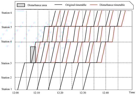
Figure 1.
The rescheduling problem when a disturbance occurs in a section.
3.3. Model Assumption
The following assumptions are made with regard to the proposed model.
- The high-speed railway system can achieve real-time and precise perception of the information of disturbance occurrence by implementing sensor networks and information fusion in complex environments.
- At each station, there are designated arrival and departure tracks for up-direction and down-direction trains, respectively. Given the similarity in the rescheduling processes for up-direction and down-direction trains, our study centers on examining the real-time rescheduling problem for a single direction.
- The train speed trajectories with different driving strategies are pre-calculated in this paper.
4. Model Formulation
4.1. Objective Function
The objective of our real-time rescheduling model is to minimize deviations from the original timetable while expediting the return to the normal timetable. To achieve this objective, we define the following optimization objectives:
4.2. Departure Time and Dwell Time Constraints
In order to allow passengers to catch the train in time, the train cannot depart the station before its planned departure time (Equation (2)). When establishing the dwell time constraint, we take into account the train stop plan as outlined in the original timetable. Specifically, if Train i is scheduled to stop at Station n, we enforce a minimum dwell time of e to allow passengers sufficient time for boarding and alighting. Conversely, if Train i does not make a stop at Station n, we set the dwell time to based on the train speed and station data.
4.3. Running Time Constraints
4.3.1. Driving Strategy
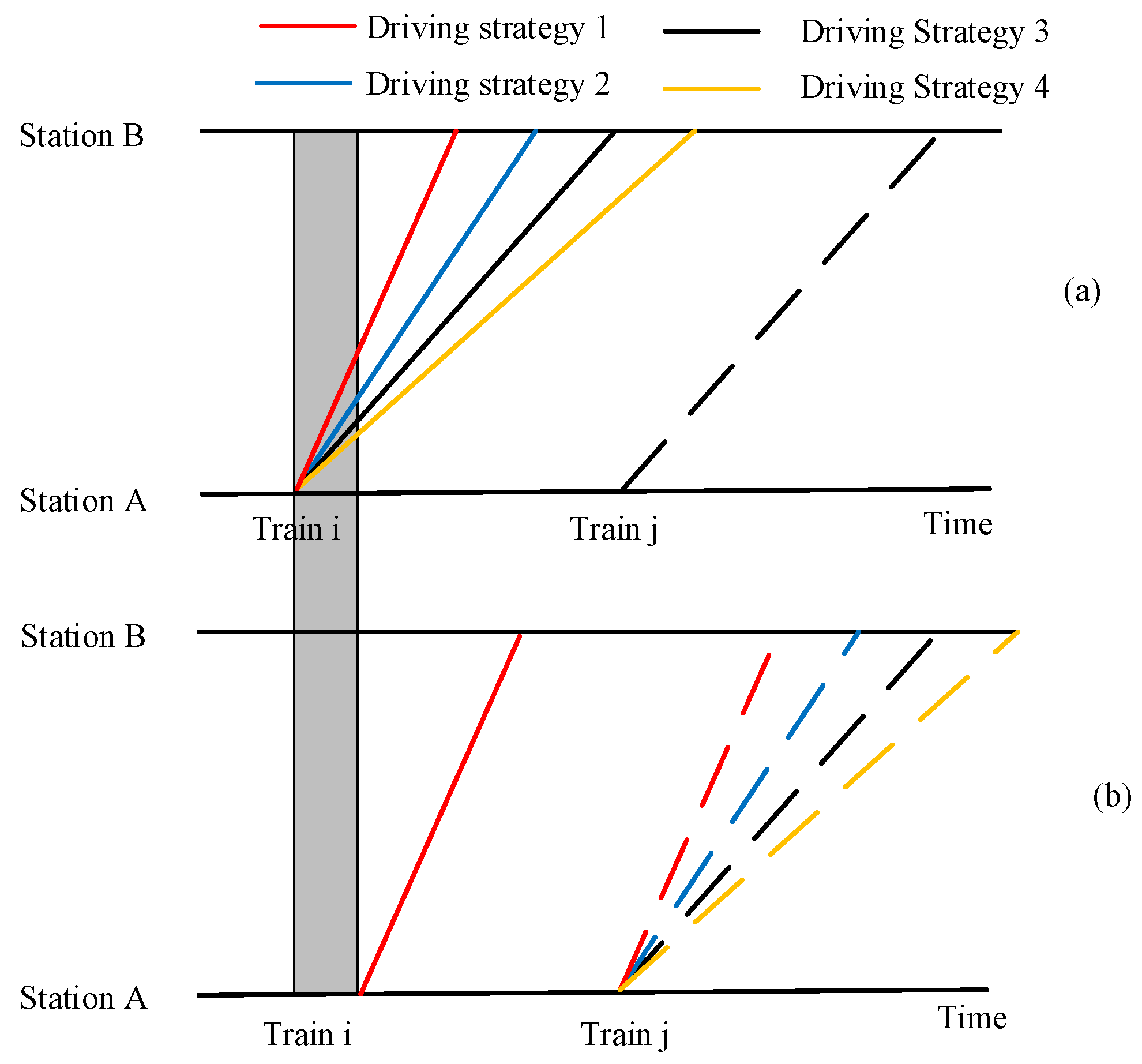
In the event of a disruption, the operational plan becomes temporarily unavailable while the ATO onboard equipment automatically defaults to a pre-selected driving strategy for controlling train operations. Additionally, the driver has the option to manually adjust the pre-selected driving strategy based on the train’s operational circumstances.
Figure 2a illustrates various driving strategies and provides an example of how these strategies can address disruptions. In Figure 2, we present four driving strategies within an inter-station context: driving strategy 1, driving strategy 2, driving strategy 3, and driving strategy 4, corresponding to the shortest running time, the second short-running time, the planned running time, and the longest running time, respectively.
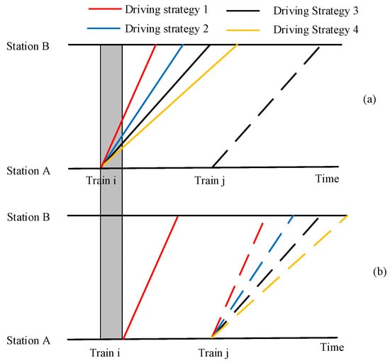
Figure 2.
Illustration of choosing different driving strategies.
In the event of a disturbance ahead of a train’s direction, as depicted in Figure 2b, train i at station n may experience a delayed departure due to equipment failure. In response, train i can opt for driving strategy 2 to minimize the delay. Train j, on the other hand, has more flexibility in responding to disruptions. It can choose driving strategy 4 to extend the running time between inter-stations, relieving station capacity stress. Alternatively, under the safety constraints, it can choose driving strategy 1 or 2 to reduce running time and energy consumption between inter-stations. Therefore, the real-time rescheduling model must account for the selection of train driving strategies.
4.3.2. Train Stop Plan
In a high-speed railway system without the ATO (Automatic Train Operation) system, train operations are manually controlled by a driver. This manual control often leads to uncertainty in the running times between stations. Previous research typically addressed this uncertainty by adding extra time to accommodate individual train stop plans.
However, with the introduction of the ATO system, the approach of simply setting additional time based on stop plans no longer satisfies the demand for promptly restoring the timetable when disruptions occur.
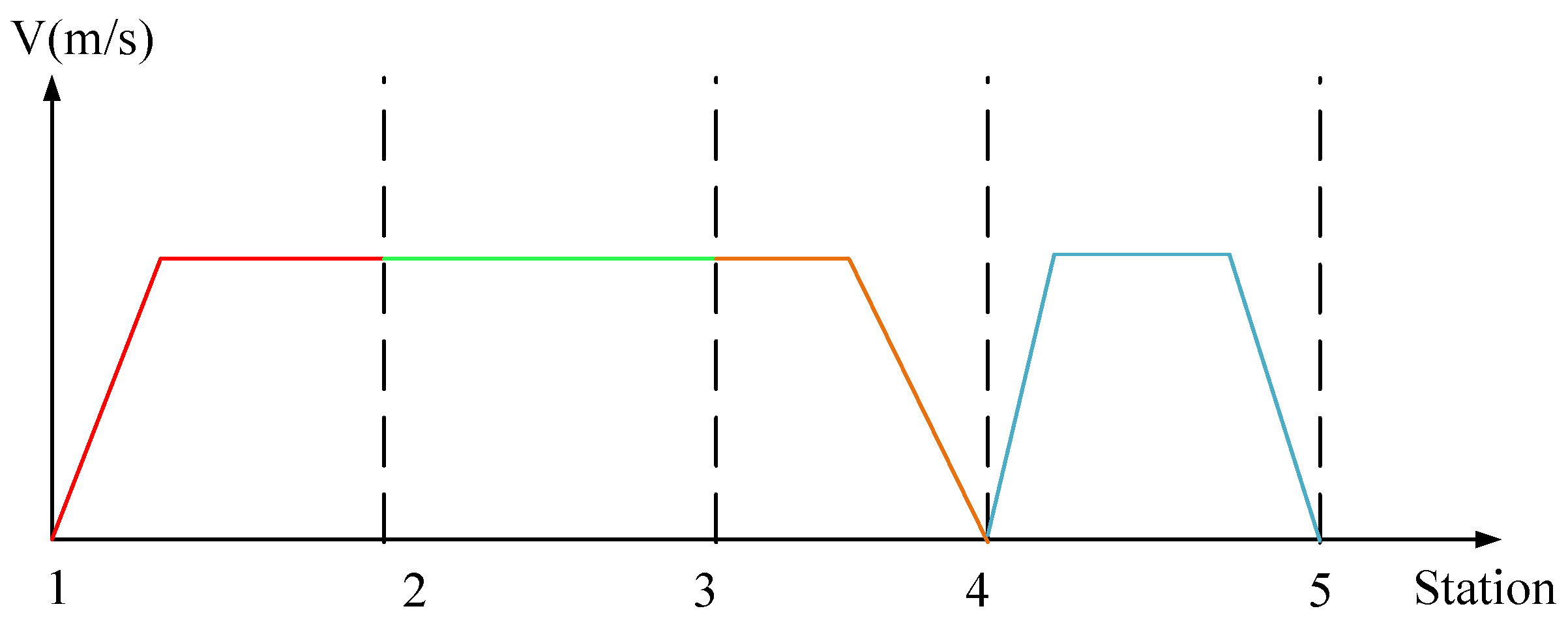
For instance, consider a train scheduled to pass through five stations but making stops only at stations 2 and 5. The speed trajectories corresponding to different stop plans are depicted in Figure 3.
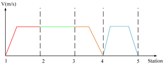
Figure 3.
Train speed trajectories with different stop plan.
In Figure 3, if the train departs from station 1 without stopping at station 2, the speed trajectory is represented by the red line. If the train departs from station 4 and stops at station 5, the train’s speed trajectory follows the blue line. Similarly, the green line and brown line represent other train stop plans alternatively.
According to the train stop plan, the train running time with a fixed driving strategy should be formulated as:
is the inter-station travel time of train i between station n and station using driving strategy l. is the stop plan of train i at station n As we mentioned above, the train running time at each inter-station is related to the train stop plan and different driving strategies (l). The train running time with a fixed driving strategy in an inter-station corresponds to different stop plans.
The linearized form of Equation (5) is as follows:
Meanwhile, the different ATO driving strategies should also be considered in our model. So, the running time constraint is:
is a binary variable, if the driving strategy of train i at inter-station s is l, , otherwise, .
4.4. Headway Constraints
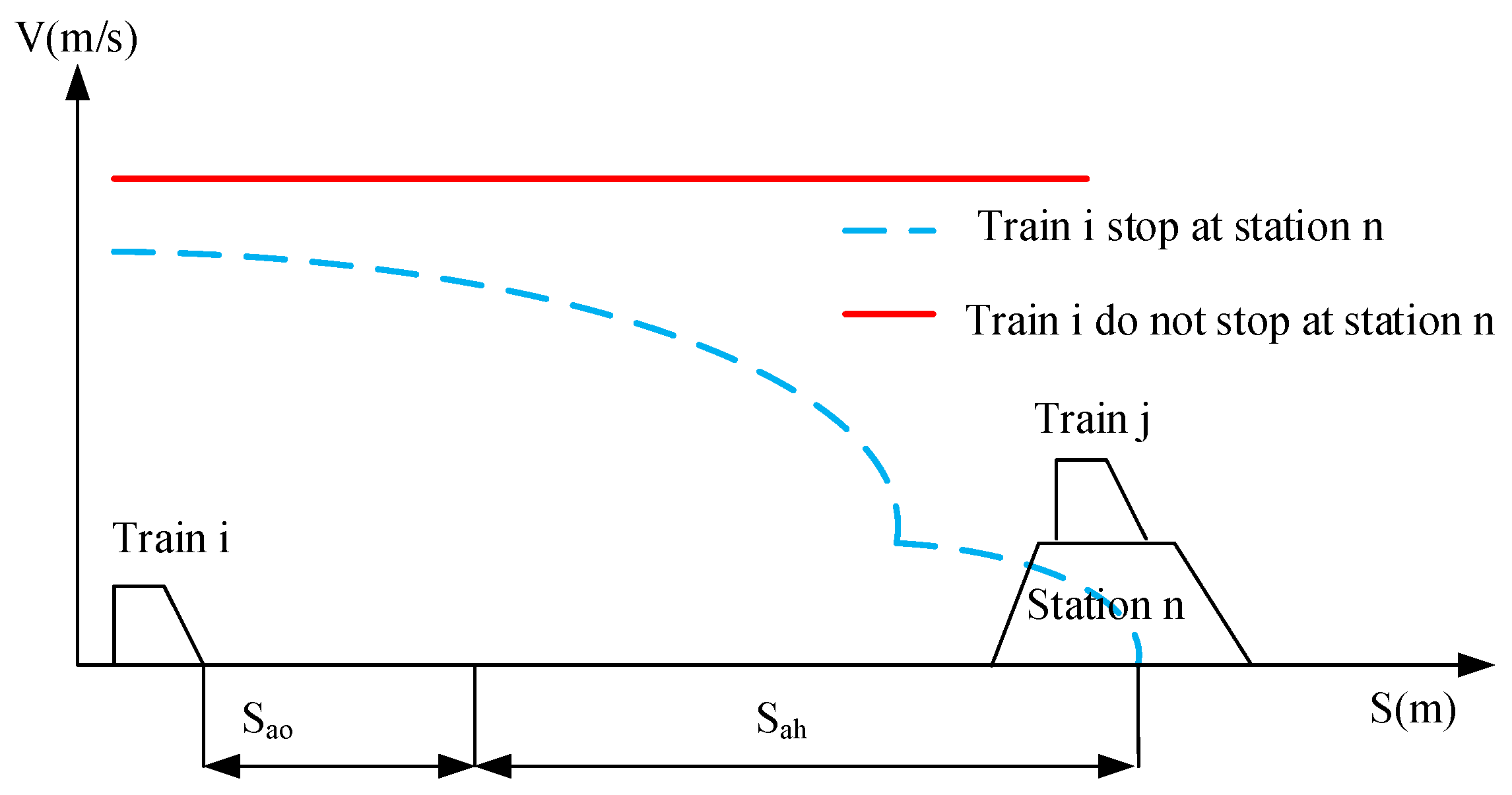
The headway between adjacent trains depends on the stop plans of these two trains. In Figure 4, we present the speed trajectory of train i as it arrives at station n, and this trajectory is determined by train i’s stop plan. Specifically, the blue dash line illustrates train i’s speed trajectory when it makes a stop at station n, while the red line depicts the speed trajectory when it does not stop at station n.
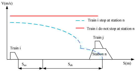
Figure 4.
Arrival Headway.
The calculation method for the minimum arrival headway between train i and train j is:
is the arrival headway. is the minimum distance between two trains. and are the distance and time that the station needs to finish the operation when a train arrives at the station.
In Equation (8), it is important to note that remains fixed to ensure that the station has sufficient time to carry out the arrival operation. The safety distance between two trains during inter-station travel is determined by the maximum speed of train i. is determined by train i’s stop plan.
Therefore, the arrival headway between train i and train j is contingent upon both the maximum speed of train i and the specific stop plan of train i. In Figure 4, train i is considered the later train while train j is the former train. However, for a comprehensive analysis that includes the arrival of a train between these two, we must also account for the scenario where train j is the later train. As a result, the minimum arrival headway between two trains can be expressed using the following equation:
is the arrival headway, is the arrival headway of train i and train j at station n when train i is the former train and does not stop at station n. is the arrival headway of train i and train j at station n when train i is the former train and stop at station n. is the arrival headway of train i and train j at station n when train j is the former train and does not stop at station n. is the arrival headway of train i and train j at station n when train j is the former train and stop at station n.
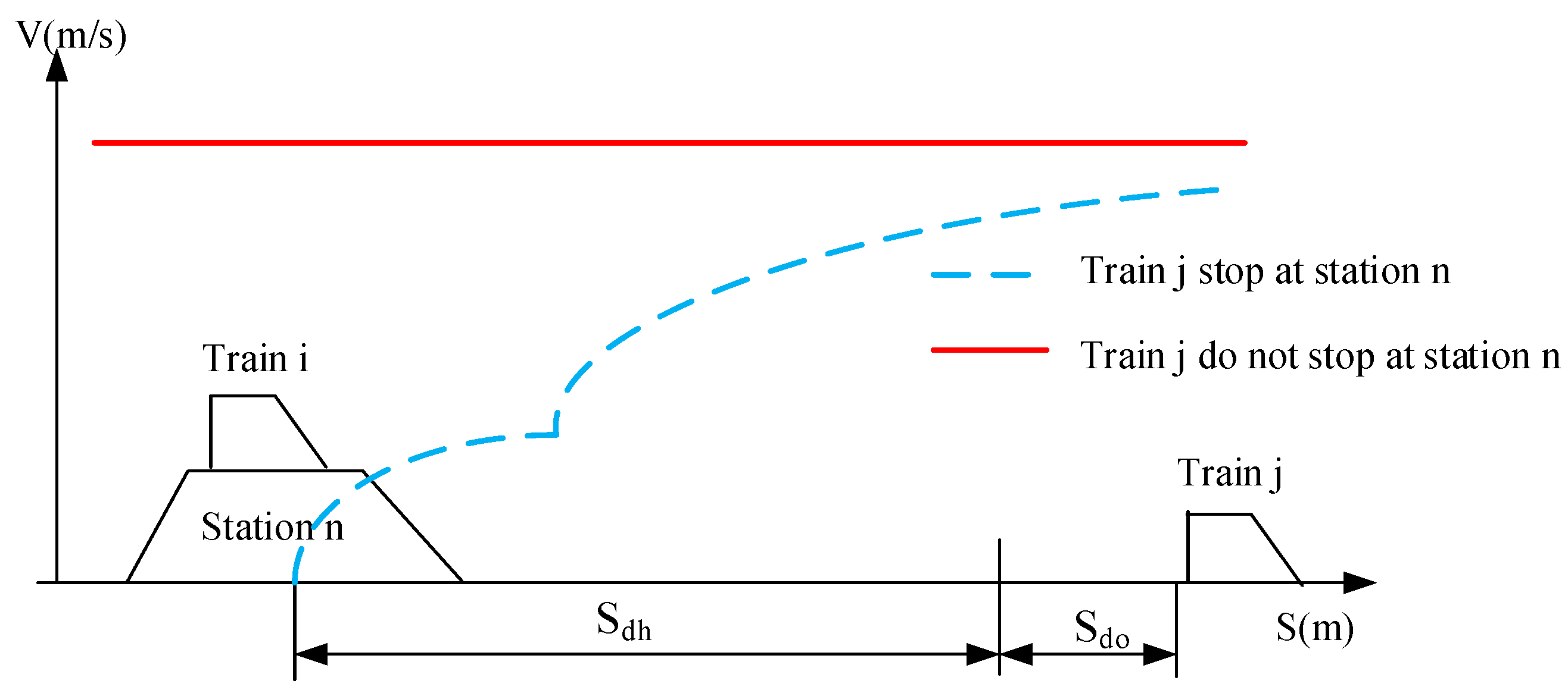
Meanwhile, the departure headway between two trains is calculated similarly to the arrival headway, but it is mainly decided by the former train stop plan. Simultaneously, the departure headway between two trains is computed in a similar manner as the arrival headway, but it primarily depends on the stop plan of the former train. In Figure 5, we illustrate the speed trajectory of train j as it departs from station n, and this trajectory is determined by train j’s stop plan at station n. The blue dash line depicts train j’s speed trajectory when it makes a stop at station n, while the red line represents the speed trajectory when it does not stop at station n.
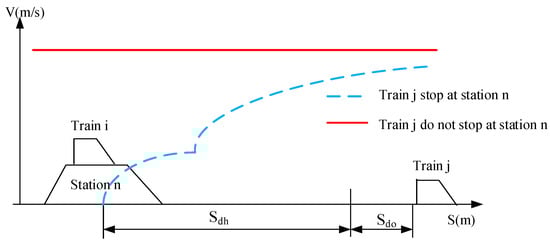
Figure 5.
Departure Headway.
The calculation method for the minimum departure headway between train i and train j is:
is the distance that train j needs to leave the station, and it is a fixed value. is also a fixed time that the station needs to complete the operations when a train departs from the station. So, the departure headway between train i and train j is related to the maximum speed of train i and the stop plan of train j. In Figure 5, train j is the former train, train i is the later train. Similar to the minimum arrival headway, the minimum departure headway is:
is the departure headway, is the departure headway of train i and train j at station n when train i is the former train and does not stop at station n. is the departure headway of train i and train j at station n when train i is the former train and stop at station n. is the departure headway of train i and train j at station n when train j is the former train and does not stop at station n. is the departure headway of train i and train j at station n when train j is the former train and stop at station n.
The headway constraint can be set as:
Equations (14) and (15) are used to determine the order of train i and train j departure from station n. is the minimum departure time. Equations (16) and (17) are used to determine the order of train i and train j arrive at station . is the minimum arrival headway. is a binary variable, which means that if the departure time of train i is later than train j at station n, .
4.5. Station Capacity Constraints
We will primarily focus on the capacity constraint of intermediate stations. To ensure compliance with the station’s capacity constraints (as defined in Equation (24)), each intermediate station must allocate a siding line for every train. In other words, when a train arrives at a station, there must be at least one siding line available for its use.
The order of train i and train j arrive and departure from station n is determined by Equations (18) and (19). is a binary variable, which means that if train i departure from station n later than train j arriving at station n, . Meanwhile, when and =1, , otherwise, (Equations (20)–(22)), which means that when train i arrive at station n, train j do not leave station n. is the number of trains that arrive and do not leave the station n when train i arrives at station n.
4.6. Real-Time Rescheduling Model
We formulate the problem described in this chapter as the following integer programming model:
s.t.
5. Case Study
The test bed we are using is a segment of the Beijing–Shanghai high-speed railway line, which happens to be one of the busiest railway lines in China. In this study, we have chosen to focus on a specific section of this railway line, running from Xuzhou East Station to Shanghai Hongqiao Station. This segment comprises 13 stations. Our primary focus is on the train traffic moving in a single direction, specifically from Xuzhou to Shanghai. It is worth noting that we are not considering the opposite direction, where trains travel from Shanghai to Nanjing. This decision is made to avoid complexities related to rolling stock circulation.
In this case, we operate under the assumption of having prior knowledge of disturbance events, which allows us to anticipate their impact on the duration and location of the disturbances. With this understanding, we establish multiple disturbance scenarios by varying the duration time of the disturbance initially. We explore the impact of disturbances by considering different duration times, ranging from 10 min, 20 min, 30 min, to 60 min. Next, we introduce variability in the locations of disturbances along the railway line. Specifically, when a disturbance occurs at station 1, we categorize the scenarios into four types based on the duration and the number of affected trains: disturbance lasting 10 min at station 1 (10,1), disturbance lasting 20 min at station 1 (20,1), disturbance lasting 30 min at station 1 (30,1), and disturbance lasting 60 min at station 1 (60,1).
In our study, we employ a highly demanding timetable. This timetable is constructed by selecting 12 consecutive trains from the real timetable. We have based our train stop plans and travel times at each station on authentic data obtained from the real timetable. Moreover, the line data used to establish various ATO driving strategies is also sourced from real-world data. The distance of each inter-station is listed in Table 2.
Table 2.
Distance of Inter-station.
In this section, three experiments are presented to verify the effectiveness of the proposed model. The simulation experiments were programmed using MATLAB R2016a, calling the commercial optimization software CPLEX 12.6.2 as a model solver, and using the YALMIP toolbox as an interface between CPLEX and MATLAB. The simulation platform is a personal computer with Windows (64-bit) operating system, where the memory is 16.00 GB and the processor is 1.6 GHz Intel Core .
In the forthcoming section on case analysis, we begin by examining how different disturbance scenarios affect train operations. This analysis will yield real-time rescheduling tailored to each disturbance scenario. Next, we evaluate the train rescheduling model under each disturbance scenario while considering various numbers of driving strategies. Our aim is to optimize train speed and efficiency. Lastly, we compare and analyze the solutions derived from our optimization model, particularly focusing on the timetable without optimization. This will help us assess the quality and effectiveness of the solutions provided by this model.
5.1. Case 1: Impact of Different Disturbance Scenarios
The real-time rescheduling problem was solved for different disturbance scenarios, and the results are shown in Table 3.
Table 3.
Rescheduling results under different disturbance scenarios.
This section assesses the adaptability of the model in solving various disturbance scenarios. To expedite the model’s solving speed, we will compare the results and precision analysis of solving with time limits set at 180 s and 360 s. The first column in the table represents disturbance scenarios, with the two numbers in parentheses indicating the disturbance duration and the station number where the disturbance occurs. The second column displays the total train delay, the third column represents the solving time, and the fourth column displays the solving gap (Table 3).
From Table 3, it is evident that when the disturbance duration is within 30 min, the algorithm’s solving error remains below 3%. When the disturbance duration extends to 60 min, all solving errors stay within 6%. In the comparison between solving times of 180 s and 360 s, when the disturbance duration is 45 min and 60 min, there is a reduction solving gap, albeit not significantly. Disturbances occurring at different locations along the railway line have varying impacts on train operations. For instance, with the same disturbance duration of 30 min, disturbances occurring at Location 1 have a more significant impact than those occurring at Location 3. However, disturbances occurring at Location 5 have a more significant impact than those occurring at Location 1. This is because disturbances occurring later when trains are approaching the terminal station have no time and space to catch the timetable.
5.2. Case 2: Evaluation of Different Driving Strategies
This section analyzes the impact of ATO driving strategies on optimization results, primarily from two aspects. First, we examine the influence of the number of pre-stored ATO driving strategies. Second, we investigate the effect of ATO’s maximum and minimum speeds on optimization results.
As mentioned in Section 5.1, disturbances have a greater impact when they occur closer to the beginning. Therefore, for this section, the station affected by disturbances is set to Station 1. The first column represents the lowest and highest speeds for ATO driving strategies. The second, third, and fourth columns display the total train delay times when the disturbance duration is 20 min for ATO driving strategy quantities of 3, 5, and 7. The fifth, sixth, and seventh columns show the total train delay times when the disturbance duration is 30 min for ATO driving strategy quantities of 3, 5, and 7 (Table 4).
Table 4.
Rescheduling results under different driving strategies.
From Table 4, it is evident that the total train delay time is primarily influenced by the maximum speed of the ATO automatic driving strategy. When the disturbance duration is 20 min, the quantity of ATO driving strategies has no impact on the total train delay time because, at this point, trains only need to select the fastest strategy. However, when the disturbance duration is 30 min, the timetable is more significantly affected by the disturbance, requiring the adjustment of inter-station travel times using non-optimal speeds. Meanwhile, an increase in the number of train driving strategies will reduce total delay, but it does not mean that the more driving strategies there are, the better. When the total delay time is optimized to a certain extent, the number of driving strategies has little impact on the reduction of total delay.
5.3. Case 3: Comparative Analysis with the Timetable without Optimization
To compare the quality of the train scheduling adjustments obtained by the model in this chapter with the timetable without optimization (TWO), this section analyzes the results of both strategies across 15 disturbance scenarios. The TWO in this context involves extending the departure times of all trains based on their delay times. The results are presented in Table 5.
Table 5.
Total delay time of different approach.
In Table 5, the first column represents the disturbance scenarios. The second and third columns display the objective function values obtained by the model presented in this chapter and the FSFS model, respectively. The fourth column shows the ratio of the total delay reduction obtained by the model in this section compared to TWO.
From Table 5, it is evident that the results obtained by the model in this chapter outperform those obtained under the TWO strategy. Compared to TWO, the objective values of the model in this chapter decrease in all disturbance scenarios. This is especially pronounced for disturbances with delays less than 10 min, where the objective function values obtained from the model decrease by almost 99%, indicating that the model presented in this paper can return trains back to their normal schedules under such circumstances. Additionally, for disturbances with delays exceeding 30 min, the total delay is reduced by over 30%.
6. Conclusions
In this paper, we conduct a comprehensive analysis of the influence of the transition to ATO system on real-time rescheduling models. Recognizing the distinct impact of the ATO system on real-time rescheduling, we introduce a mixed-integer linear programming model that encompasses train re-timing, reordering, and the minimization of passenger delays. The primary objective of this model is to minimize train delay times.
We investigate the effects of various disturbance scenarios and different driving strategies on real-time rescheduling problems. The results demonstrate the efficiency and effectiveness of our model in resolving a wide range of disturbance scenarios. Furthermore, we found that the total delay time of trains is primarily determined by the maximum speed of the ATO system. Depending on the duration of the disturbance, the number of ATO driving strategies has varying effects on the overall delay time. Specifically, when the disturbance duration falls within a certain range, the number of ATO driving strategies has no impact on the total delay time. When the disturbance duration is excessively long, the number of ATO driving strategies does have a certain influence on the total delay time. An increase in the number of train driving strategies will reduce delay time, but it does not mean that the more driving strategies there are, the better. When the total delay time is optimized to a certain extent, the number of driving strategies has little impact on the reduction in total delay time. Compared with the timetable without optimization, our model can significantly reduce the total delay.
Author Contributions
F.L.: Conceptualization, Methodology, Software, Writing—original draft. J.X.: Conceptualization, Methodology, Writing—review and editing. All authors have read and agreed to the published version of the manuscript.
Funding
This research was funded by the National Natural Science Foundation of China under Grant (No.62073026).
Data Availability Statement
Not applicable.
Acknowledgments
The authors would like to express their gratitude to Xie Lijun and Fu Minxue for their assistance in reviewing and editing this paper. Additionally, we extend our appreciation to the anonymous referees and the editor for their valuable comments and suggestions.
Conflicts of Interest
The authors declare no conflict of interest.
References
- Corman, F.; Meng, L. A review of online dynamic models and algorithms for railway traffic management. IEEE Trans. Intell. Transp. Syst. 2014, 16, 1274–1284. [Google Scholar] [CrossRef]
- Cacchiani, V.; Huisman, D.; Kidd, M.; Kroon, L.; Toth, P.; Veelenturf, L.; Wagenaar, J. An overview of recovery models and algorithms for real-time railway rescheduling. Transp. Res. Part B Methodol. 2014, 63, 15–37. [Google Scholar]
- Fang, W.; Yang, S.; Yao, X. A survey on problem models and solution approaches to rescheduling in railway networks. IEEE Trans. Intell. Transp. Syst. 2015, 16, 2997–3016. [Google Scholar]
- Dorfman, M.; Medanic, J. Scheduling trains on a railway network using a discrete event model of railway traffic. Transp. Res. Part B Methodol. 2004, 38, 81–98. [Google Scholar] [CrossRef]
- Törnquist, J.; Persson, J.A. N-tracked railway traffic re-scheduling during disturbances. Transp. Res. Part B Methodol. 2007, 41, 342–362. [Google Scholar] [CrossRef]
- D’Ariano, A.; Pacciarelli, D.; Pranzo, M. A branch and bound algorithm for scheduling trains in a railway network. Eur. J. Oper. Res. 2007, 183, 643–657. [Google Scholar]
- Schöbel, A. A model for the delay management problem based on mixed-integer-programming. Electron. Notes Theor. Comput. Sci. 2001, 50, 1–10. [Google Scholar] [CrossRef]
- Duendar, S.; Sahin, I. Train re-scheduling with genetic algorithms and artificial neural networks for single-track railways. Transp. Res. Part C Emerg. Technol. 2013, 27, 1–15. [Google Scholar] [CrossRef]
- Corman, F.; D’Ariano, A.; Pacciarelli, D.; Pranzo, M. A tabu search algorithm for rerouting trains during rail operations. Transp. Res. Part B Methodol. 2010, 44, 175–192. [Google Scholar] [CrossRef]
- Lamorgese, L.; Mannino, C. The track formulation for the train dispatching problem. Electron. Notes Discret. Math. 2013, 41, 559–566. [Google Scholar] [CrossRef]
- Meng, L.; Zhou, X. Robust single-track train dispatching model under a dynamic and stochastic environment: A scenario-based rolling horizon solution approach. Transp. Res. Part B 2011, 45, 1080–1102. [Google Scholar] [CrossRef]
- Yang, L.; Zhou, X.; Gao, Z. Credibility-based rescheduling model in a double-track railway network: A fuzzy reliable optimization approach. Omega 2014, 48, 75–93. [Google Scholar] [CrossRef]
- Pellegrini, P.; Marlière, G.; Rodriguez, J. Optimal train routing and scheduling for managing traffic perturbations in complex junctions. Transp. Res. Part B Methodol. 2014, 59, 58–80. [Google Scholar] [CrossRef]
- Zhan, S.; Kroon, L.G.; Veelenturf, L.P.; Wagenaar, J.C. Real-time high-speed train rescheduling in case of a complete blockage. Transp. Res. Part B Methodol. 2015, 78, 182–201. [Google Scholar] [CrossRef]
- Xu, P.; Corman, F.; Peng, Q.; Luan, X. A train rescheduling model integrating speed management during disruptions of high-speed traffic under a quasi-moving block system. Transp. Res. Part B Methodol. 2017, 104, 638–666. [Google Scholar] [CrossRef]
- Wang, P.; Goverde, R.M. Multi-train trajectory optimization for energy efficiency and delay recovery on single-track railway lines. Transp. Res. Part B Methodol. 2017, 105, 340–361. [Google Scholar] [CrossRef]
- Wu, W.; Liu, R.; Jin, W. Modelling bus bunching and holding control with vehicle overtaking and distributed passenger boarding behaviour. Transp. Res. Part B Methodol. 2017, 104, 175–197. [Google Scholar] [CrossRef]
- Luan, X.; Wang, Y.; De Schutter, B.; Meng, L.; Lodewijks, G.; Corman, F. Integration of real-time traffic management and train control for rail networks—Part 1: Optimization problems and solution approaches. Transp. Res. Part B Methodol. 2018, 115, 41–71. [Google Scholar] [CrossRef]
- Liu, F.; Xun, J.; Liu, R.; Yin, J.; Dong, H. A real-Time rescheduling approach using loop iteration for high-Speed railway traffic. IEEE Intell. Transp. Syst. Mag. 2023, 15, 318–332. [Google Scholar] [CrossRef]
- Wu, W.; Lin, Y.; Liu, R.; Jin, W. The multi-depot electric vehicle scheduling problem with power grid characteristics. Transp. Res. Part B Methodol. 2022, 155, 322–347. [Google Scholar] [CrossRef]
- Zhan, S.; Wong, S.; Shang, P.; Lo, S. Train rescheduling in a major disruption on a high-speed railway network with seat reservation. Transp. A Transp. Sci. 2022, 18, 532–567. [Google Scholar] [CrossRef]
- Yuan, J.; Jones, D.; Nicholson, G. Flexible real-time railway crew rescheduling using depth-first Search. J. Rail Transp. Plan. Manag. 2022, 24, 100353. [Google Scholar] [CrossRef]
- Liu, F.; Xun, J.; Zhou, M.; He, S.; Dong, H. A driving strategy based integrated rescheduling Model for high-Speed railway by using the parallel intelligent method. In Proceedings of the 2022 IEEE 2nd International Conference on Digital Twins and Parallel Intelligence (DTPI), Boston, MA, USA, 24–28 October 2022. [Google Scholar]
- Zhang, C.; Gao, Y.; Cacchiani, V.; Yang, L.; Gao, Z. Train rescheduling for large-scale disruptions in a large-scale railway network. Transp. Res. Part B Methodol. 2023, 174, 102786. [Google Scholar] [CrossRef]
Disclaimer/Publisher’s Note: The statements, opinions and data contained in all publications are solely those of the individual author(s) and contributor(s) and not of MDPI and/or the editor(s). MDPI and/or the editor(s) disclaim responsibility for any injury to people or property resulting from any ideas, methods, instructions or products referred to in the content. |
© 2023 by the authors. Licensee MDPI, Basel, Switzerland. This article is an open access article distributed under the terms and conditions of the Creative Commons Attribution (CC BY) license (https://creativecommons.org/licenses/by/4.0/).