
An Integrated Method for Reducing Arrival Interval by Optimizing Train Operation and Route Setting
 , ,
, ,  ,
, 
Abstract
:1. Introduction
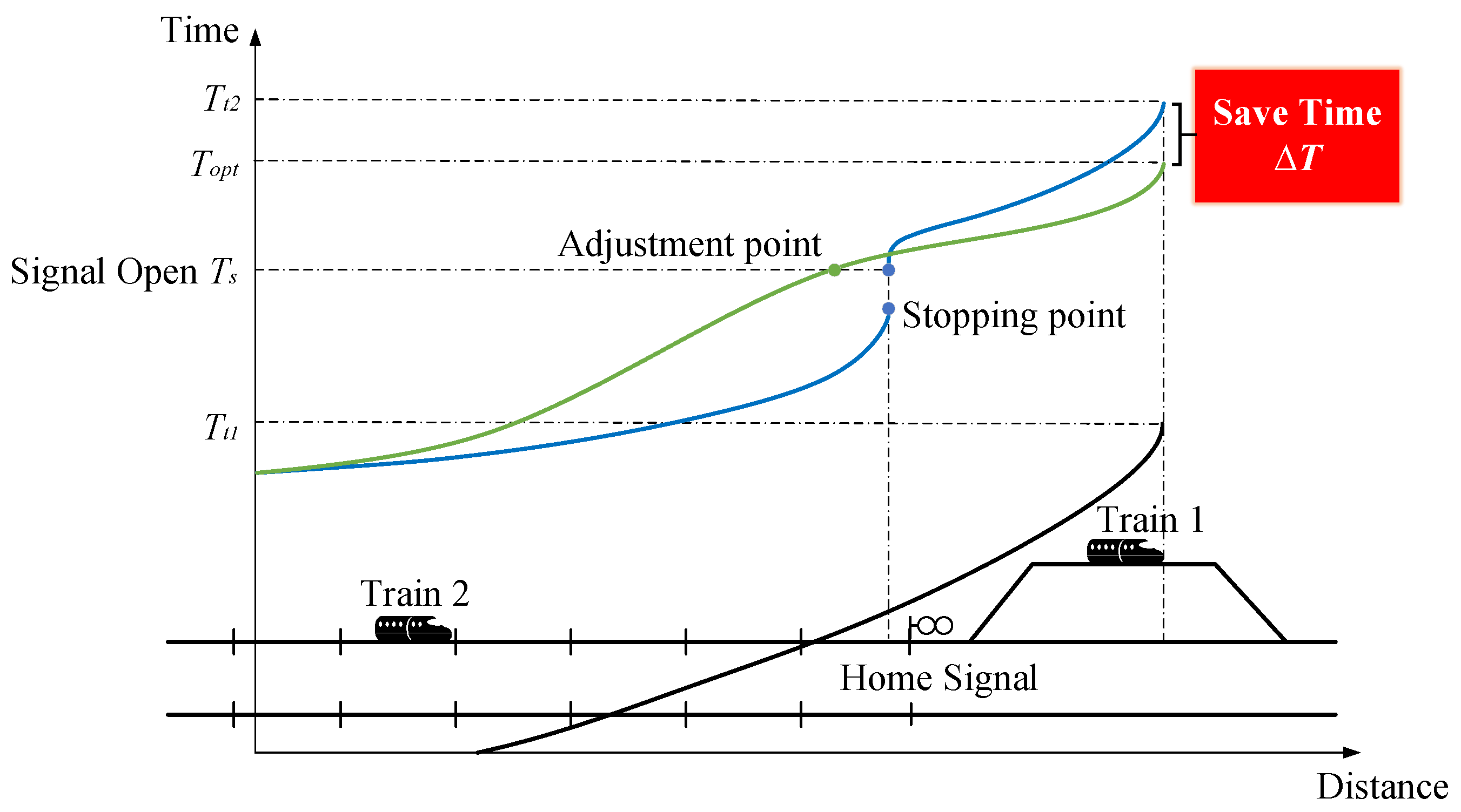
- We construct an integrated operation method to compress the arrival interval for the entry conflict scenario. This approach improves the passing speed by analyzing three entry strategies to avoid unnecessary stops in the throat area.
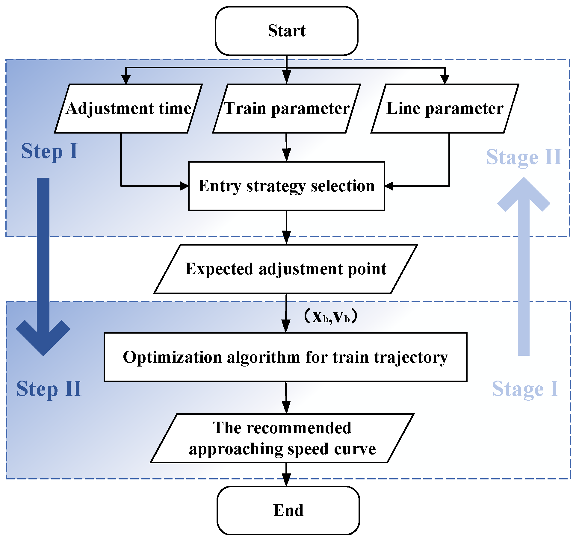
- The two-step method consists of mathematical analysis and optimization algorithms, with the former used to determine the entry operation strategy and the latter for calculating the optimal adjustment trajectory.
- The improved intelligent optimization algorithm can solve the recommended trajectory in a short period of time after obtaining the adjustment time. In addition, the validity and feasibility of the method are verified by simulation experiment and field test.
2. Related Work
3. Problem Formulation
3.1. Normal Operation Scenario
3.2. Optimal Operation Scenario
4. An Integrated Operation Method for Reducing Arrival Interval of Trains
4.1. Analysis of the Entry Operation Strategy
- The acceleration and deceleration process is an ideal uniform variable speed process.
- The endpoint of the planned entry running curve is at position in Figure 4.
- The platform length allows the train to reach the speed limit in the throat area and cruise in either pattern.
- To simplify the train speed profile optimization model, there are no other temporary speed limits between stations, and the line speed limit is uniformly .
- The introduction of the strategy of an operation mainly ignores the interlocking mechanism in the throat area, assuming that the receiving path is locked and released as a single entity.
4.1.1. Pattern of MA-CR-MB
4.1.2. Pattern of MA-MB
4.1.3. Pattern of MA
4.2. Analysis of the Optimal Adjustment Trajectory
4.2.1. The Improved Meta-Heuristic Algorithm
- (1)
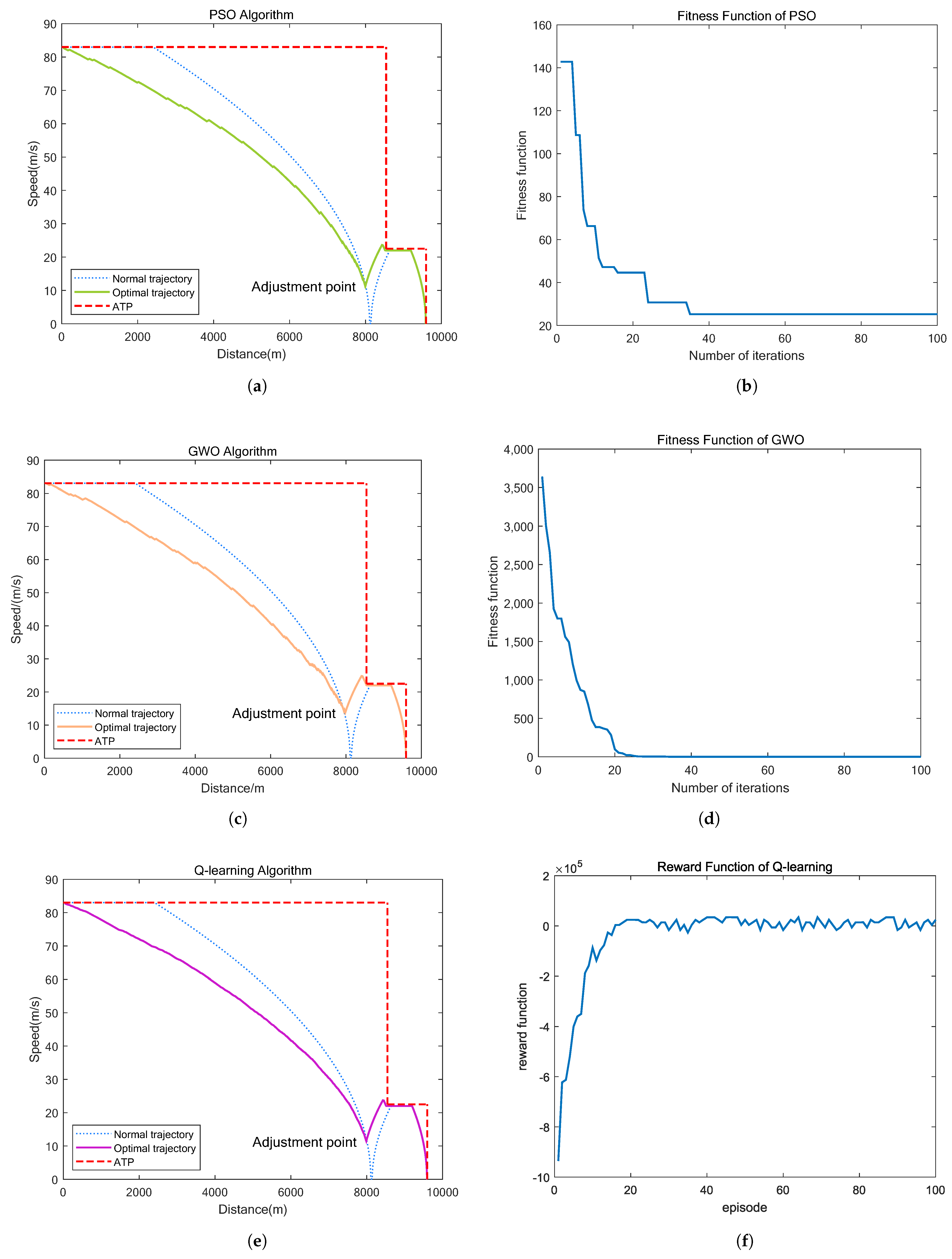
- PSO Algorithm
- (2)
- GWO Algorithm
- Tracking, chasing and approaching the prey;
- Chasing and encircling the prey and harassing until it stops moving;
- Attacking the prey.
| Algorithm 1 The improved meta-heuristic algorithms |
|
4.2.2. The Improved Q-Learning Algorithm (Algorithm 2)
| Algorithm 2 The improved Q-learning algorithm |
|
5. Experimental Results
5.1. Case Study 1: The Train Speed Profile Optimization Model Based with Simulation Line for Succeeding Train
- Average running time error (Runtime_error_avg): It computes the average absolute deviation of the running time from the target value of 170 s, but only for valid solutions.
- Average target speed error (Speed_error_avg): It calculates the average absolute deviation of the speed from the target value for valid solutions.
- Average target location error (Location_error_avg): It calculates the average absolute deviation of the place from the target value for valid solutions.
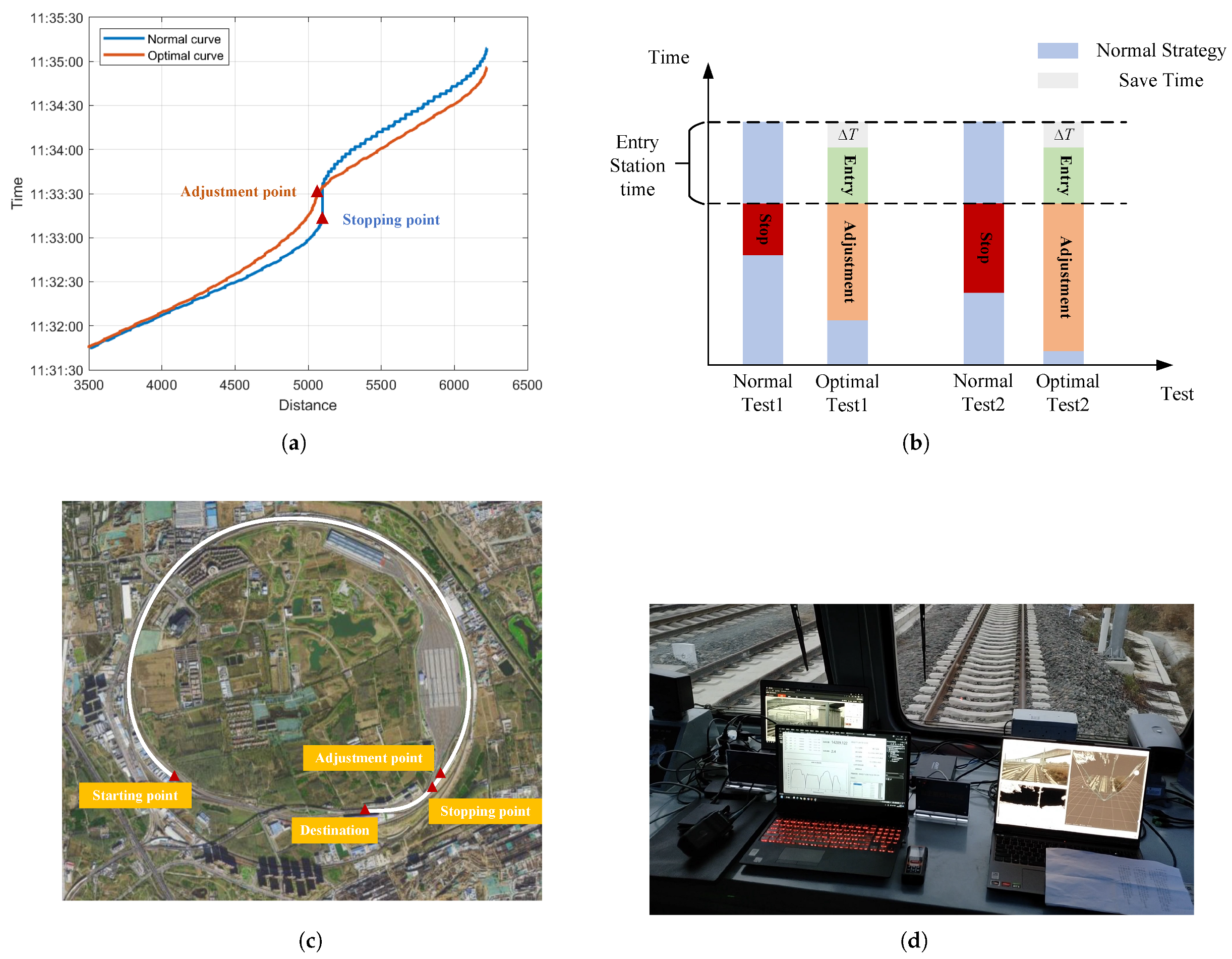
5.2. Case Study 2: Exploration of the Integrated Method for Succeeding Train Based on Field Test
6. Conclusions and Future Work
Author Contributions
Funding
Data Availability Statement
Conflicts of Interest
References
- Corman, F.; D’Ariano, A.; Pacciarelli, D.; Pranzo, M. Evaluation of green wave policy in real-time railway traffic management. Transp. Res. Part C Emerg. Technol. 2009, 17, 607–616. [Google Scholar] [CrossRef]
- Xun, J.; Tang, T.; Ning, B. Optimization of speed profile for delayed train entering station. In Proceedings of the 2011 IEEE International Conference on Service Operations, Logistics and Informatics, Beijing, China, 10–12 July 2011; pp. 428–433. [Google Scholar] [CrossRef]
- Albrecht, T. The Influence of Anticipating Train Driving on the Dispatching Process in Railway Conflict Situations. Netw. Spat. Econ. 2009, 9, 85–101. [Google Scholar] [CrossRef]
- Yun, B.; Tinkin, H.; Baohua, M. Train Control to Reduce Delays upon Service Disturbances at Railway Junctions. J. Transp. Syst. Eng. Inf. Technol. 2011, 11, 114–122. [Google Scholar] [CrossRef]
- Fu, L.; Dessouky, M. Models and algorithms for dynamic headway control. Comput. Ind. Eng. 2017, 103, 271–281. [Google Scholar] [CrossRef]
- Cacchiani, V.; Huisman, D.; Kidd, M.; Kroon, L.; Toth, P.; Veelenturf, L.; Wagenaar, J. An overview of recovery models and algorithms for real-time railway rescheduling. Transp. Res. Part B Methodol. 2014, 63, 15–37. [Google Scholar] [CrossRef]
- Zhu, Y.; Goverde, R.M.P. Dynamic and robust timetable rescheduling for uncertain railway disruptions. J. Rail Transp. Plan. Manag. 2020, 15, 100196. [Google Scholar] [CrossRef]
- Dong, H.R.; Liu, X.; Zhou, M.; Zheng, W.; Xun, J.; Gao, S.G.; Song, H.F.; Li, Y.D.; Wang, F.Y. Integration of Train Control and Online Rescheduling for High-Speed Railways in Case of Emergencies. IEEE Trans. Comput. Soc. Syst. 2022, 9, 1574–1582. [Google Scholar] [CrossRef]
- Hou, L.S.; Tong, L.; Chen, J.H.; Tang, J.J.; Zhou, X.S. Joint optimization of high-speed train timetables and speed profiles: A unified modeling approach using space-time-speed grid networks. Transp. Res. Part B Methodol. 2017, 97, 157–181. [Google Scholar] [CrossRef]
- Long, S.H.; Meng, L.Y.; Wang, Y.H.; Miao, J.R.; Luan, X.J. Integrated optimization of train rescheduling decisions and train speeds based on satisfactory optimization for high-speed railway. In Proceedings of the IEEE 25th International Conference on Intelligent Transportation Systems (ITSC), Macau, China, 8–12 October 2022; pp. 4117–4123. [Google Scholar] [CrossRef]
- Ning, L.B.; Li, Y.D.; Zhou, M.; Song, H.F.; Dong, H.R. A Deep Reinforcement Learning Approach to High-speed Train Timetable Rescheduling under Disturbances. In Proceedings of the IEEE Intelligent Transportation Systems Conference (ITSC), Auckland, New Zealand, 27–30 October 2019; pp. 3469–3474. [Google Scholar] [CrossRef]
- Zhou, X.Z.; Zhang, Q.; Wang, T. Intelligent Rescheduling Research on Train Dispatching Section of Main Line High-speed Railway Based on Improved GWO Algorithm. In Proceedings of the IEEE 5th International Conference on Intelligent Transportation Engineering (ICITE), Beijing, China, 11–13 September 2020; pp. 195–199. [Google Scholar] [CrossRef]
- Jia, X.G.; Zhou, X.B.; Bao, J.; Zhai, G.Y.; Yan, R. Fusion Swarm-Intelligence-Based Decision Optimization for Energy-Efficient Train-Stopping Schemes. Appl. Sci. 2023, 13, 1497. [Google Scholar] [CrossRef]
- Duan, B.S.; Guo, C.Q.; Liu, H. A hybrid genetic-particle swarm optimization algorithm for multi-constraint optimization problems. Soft Comput. 2022, 26, 11695–11711. [Google Scholar] [CrossRef]
- Yang, W.L.; Jiang, P.; Song, S.J. High-speed Train Timetabling Based on Reinforcement Learning. In Proceedings of the IEEE Symposium Series on Computational Intelligence (IEEE SSCI), Singapore, 4–7 December 2022; pp. 1187–1193. [Google Scholar] [CrossRef]
- Zhang, Q.C.; Lin, M.; Yang, L.T.; Chen, Z.K.; Khan, S.U.; Li, P. A Double Deep Q-Learning Model for Energy-Efficient Edge Scheduling. IEEE Trans. Serv. Comput. 2019, 12, 739–749. [Google Scholar] [CrossRef]
- D’Ariano, A.; Pranzo, M.; Hansen, I.A. Conflict resolution and train speed coordination for solving real-time timetable perturbations. IEEE Trans. Intell. Transp. Syst. 2007, 8, 208–222. [Google Scholar] [CrossRef]
- D’Ariano, A.; Pacciarelli, D.; Pranzo, M. A branch and bound algorithm for scheduling trains in a railway network. Eur. J. Oper. Res. 2007, 183, 643–657. [Google Scholar] [CrossRef]
- Galapitage, A.; Albrecht, A.R.; Pudney, P.; Vu, X.; Zhou, P. Optimal real-time junction scheduling for trains with connected driver advice systems. J. Rail Transp. Plan. Manag. 2018, 8, 29–41. [Google Scholar] [CrossRef]
- Zhang, D.L.; Peng, Y.J.; Zhang, Y.M.; Wu, D.H.; Wang, H.W.; Zhang, H.L. Train Time Delay Prediction for High-Speed Train Dispatching Based on Spatio-Temporal Graph Convolutional Network. IEEE Trans. Intell. Transp. Syst. 2022, 23, 2434–2444. [Google Scholar] [CrossRef]
- Liu, Y.F.; Zhou, Y.; Su, S.; Xun, J.; Tang, T. An analytical optimal control approach for virtually coupled high-speed trains with local and string stability. Transp. Res. Part C Emerg. Technol. 2021, 125, 19. [Google Scholar] [CrossRef]
- Cao, Y.; Zhang, Z.; Cheng, F.; Su, S. Trajectory Optimization for High-Speed Trains via a Mixed Integer Linear Programming Approach. IEEE Trans. Intell. Transp. Syst. 2022, 23, 17666–17676. [Google Scholar] [CrossRef]
- Wang, Y.H.; De Schutter, B.; van den Boom, T.J.J.; Ning, B. Optimal trajectory planning for trains under fixed and moving signaling systems using mixed integer linear programming. Control Eng. Pract. 2014, 22, 44–56. [Google Scholar] [CrossRef]
- Wang, Y.H.; Zhao, K.Q.; D’Ariano, A.; Niu, R.; Li, S.K.; Luan, X.J. Real-time integrated train rescheduling and rolling stock circulation planning for a metro line under disruptions. Transp. Res. Part B Methodol. 2021, 152, 87–117. [Google Scholar] [CrossRef]
- Xu, P.J.; Corman, F.; Peng, Q.Y.; Luan, X.J. A train rescheduling model integrating speed management during disruptions of high-speed traffic under a quasi-moving block system. Transp. Res. Part B Methodol. 2017, 104, 638–666. [Google Scholar] [CrossRef]
- Wong, K.K.; Ho, T.K. Dynamic coast control of train movement with genetic algorithm. Int. J. Syst. Sci. 2004, 35, 835–846. [Google Scholar] [CrossRef]
- Sama, M.; Pellegrini, P.; D’Ariano, A.; Rodriguez, J.; Pacciarelli, D. Ant colony optimization for the real-time train routing selection problem. Transp. Res. Part B Methodol. 2016, 85, 89–108. [Google Scholar] [CrossRef]
- Sama, M.; D’Ariano, A.; Corman, F.; Pacciarelli, D. variable neighbourhood search for fast train scheduling and routing during disturbed railway traffic situations. Comput. Oper. Res. 2017, 78, 480–499. [Google Scholar] [CrossRef]
- Krasemann, J.T. Design of an effective algorithm for fast response to the re-scheduling of railway traffic during disturbances. Transp. Res. Part C Emerg. Technol. 2012, 20, 62–78. [Google Scholar] [CrossRef]
- Yu, S.P.; Lin, B.; Zhang, T.; Dai, X.W.; Liu, Q. Dynamic Scheduling Method of High-speed Trains Based on Improved Particle Swarm Optimization. In Proceedings of the International Conference on Intelligent Rail Transportation (ICIRT), Singapore, 12–14 December 2018. [Google Scholar] [CrossRef]
- Albrecht, A.; Howlett, P.; Pudney, P.; Vu, X.; Zhou, P. The two-train separation problem on non-level track-driving strategies that minimize total required tractive energy subject to prescribed section clearance times. Transp. Res. Part B Methodol. 2018, 111, 135–167. [Google Scholar] [CrossRef]
- Semrov, D.; Marsetic, R.; Zura, M.; Todorovski, L.; Srdic, A. Reinforcement learning approach for train rescheduling on a single-track railway. Transp. Res. Part B Methodol. 2016, 86, 250–267. [Google Scholar] [CrossRef]
- Su, B.Y.; Tang, T.; Su, S.; Wang, Z.K.; Wang, X.K. Integrated rescheduling of train timetables and rolling stock circulation for metro line disturbance management: A Q-learning-based approach. Eng. Optimiz. 2023, 1–24. [Google Scholar] [CrossRef]
- Albrecht, A.R.; Howlett, P.G.; Pudney, P.J.; Vu, X. Energy-efficient train control: From local convexity to global optimization and uniqueness. Automatica 2013, 49, 3072–3078. [Google Scholar] [CrossRef]
- Dokeroglu, T.; Sevinc, E.; Kucukyilmaz, T.; Cosar, A. A survey on new generation meta-heuristic algorithms. Comput. Ind. Eng. 2019, 137, 29. [Google Scholar] [CrossRef]
- Mirjalili, S.; Mirjalili, S.M.; Lewis, A. Grey Wolf Optimizer. Adv. Eng. Softw. 2014, 69, 46–61. [Google Scholar] [CrossRef]


| Items | Symbol | Unit |
|---|---|---|
| Position of signal | m | |
| Position of entry station | m | |
| Length of line | m | |
| The current location | m | |
| The current speed | m/s | |
| Station speed limit | m/s | |
| Line speed limit | m/s | |
| Speed of intersection point in MA-MB | m/s | |
| Train traction acceleration | m/s | |
| Train braking deceleration | m/s | |
| Entry running time of Pattern i | (i = 1, 2, 3) | s |
| Time saved of Pattern i | (i = 1, 2, 3) | s |
| Original entry running time | (i = 1, 2, 3) | s |
| Coding of | Working Condition |
|---|---|
| 0 | 100% Braking |
| 1 | 80% Braking |
| 2 | 60% Braking |
| 3 | 100% Tracking |
| 4 | 80% Tracking |
| 5 | 60% Tracking |
| 6 | Cruising |
| Category | Items | Symbol | Value | Unit |
|---|---|---|---|---|
| Line parameters | Station speed limit | 22 | m/s | |
| Line speed limit | 83 | m/s | ||
| Train traction acceleration | 0.5 | m/s | ||
| Train braking deceleration | 0.6 | m/s | ||
| Length of line | 9594 | m | ||
| Length of throat area | 400 | m | ||
| Length of station | 1450 | m | ||
| Initial train position | 0 | m | ||
| The adjustment time | 170 | s | ||
| PSO | The population quantity | 40 | / | |
| The maximum iteration | 100 | / | ||
| The inertia weight of PSO | w | 0.5 | / | |
| The learning factors of PSO | 0.4 | / | ||
| GWO | The population quantity | 40 | / | |
| The maximum iteration | 100 | / | ||
| Q-learning | The learning factor | 0.2 | / | |
| The discount factor | 0.9 | / | ||
| The initial epsilon | 1 | / | ||
| The epsilon decay factor | 0.82 | / | ||
| The episode maximum | 100 | / |
| MAE | Location_error_avg | Speed_error_avg | Runtime_error_avg | |
|---|---|---|---|---|
| Algorithm | ||||
| PSO | 0.174 | 1.151 | 0.032 | |
| GWO | 0.773 | 0.386 | 0.054 | |
| Q-learning | 4.055 | 2.470 | 1.003 | |
Disclaimer/Publisher’s Note: The statements, opinions and data contained in all publications are solely those of the individual author(s) and contributor(s) and not of MDPI and/or the editor(s). MDPI and/or the editor(s) disclaim responsibility for any injury to people or property resulting from any ideas, methods, instructions or products referred to in the content. |
© 2023 by the authors. Licensee MDPI, Basel, Switzerland. This article is an open access article distributed under the terms and conditions of the Creative Commons Attribution (CC BY) license (https://creativecommons.org/licenses/by/4.0/).
Share and Cite
Wu, W.; Xun, J.; Yin, J.; He, S.; Song, H.; Zhao, Z.; Hao, S. An Integrated Method for Reducing Arrival Interval by Optimizing Train Operation and Route Setting. Mathematics 2023, 11, 4287. https://doi.org/10.3390/math11204287
Wu W, Xun J, Yin J, He S, Song H, Zhao Z, Hao S. An Integrated Method for Reducing Arrival Interval by Optimizing Train Operation and Route Setting. Mathematics. 2023; 11(20):4287. https://doi.org/10.3390/math11204287
Chicago/Turabian StyleWu, Wenxing, Jing Xun, Jiateng Yin, Shibo He, Haifeng Song, Zicong Zhao, and Shicong Hao. 2023. "An Integrated Method for Reducing Arrival Interval by Optimizing Train Operation and Route Setting" Mathematics 11, no. 20: 4287. https://doi.org/10.3390/math11204287
APA StyleWu, W., Xun, J., Yin, J., He, S., Song, H., Zhao, Z., & Hao, S. (2023). An Integrated Method for Reducing Arrival Interval by Optimizing Train Operation and Route Setting. Mathematics, 11(20), 4287. https://doi.org/10.3390/math11204287