Article

Estimation and Inference for Spatio-Temporal Single-Index Models

1
School of Statistics and Data Science, Nanjing Audit University, Nanjing 211815, China
2
Department of Statistics, Florida State University, Tallahassee, FL 32306, USA
*
Author to whom correspondence should be addressed.
Mathematics 2023, 11(20), 4289; https://doi.org/10.3390/math11204289
Submission received: 17 August 2023 / Revised: 18 September 2023 / Accepted: 12 October 2023 / Published: 14 October 2023
(This article belongs to the Special Issue Statistical Modeling for Analyzing Data with Complex Structures)

Abstract

:
To better fit the actual data, this paper will consider both spatio-temporal correlation and heterogeneity to build the model. In order to overcome the “curse of dimensionality” problem in the nonparametric method, we improve the estimation method of the single-index model and combine it with the correlation and heterogeneity of the spatio-temporal model to obtain a good estimation method. In this paper, assuming that the spatio-temporal process obeys the α mixing condition, a nonparametric procedure is developed for estimating the variance function based on a fully nonparametric function or dimensional reduction structure, and the resulting estimator is consistent. Then, a reweighting estimation of the parametric component can be obtained via taking the estimated variance function into account. The rate of convergence and the asymptotic normality of the new estimators are established under mild conditions. Simulation studies are conducted to evaluate the efficacy of the proposed methodologies, and a case study about the estimation of the air quality evaluation index in Nanjing is provided for illustration.

1. Introduction

Recently, statistical analysis of spatio-temporal data has been widely used in environmental science, economics and social science, and other fields, and it plays an important role in both academic and industrial circles. Spatio-temporal data estimation methods have also been developed. Spatio-temporal correlation and spatio-temporal heterogeneity are two significant features of spatio-temporal data.
In the process of solving practical problems, spatio-temporal data models usually consider these two properties. Various spatio-temporal modeling methods have been applied to explore the effect of spatio-temporal correlation and heterogeneity. For example, ref. [1] proposed multiscale geographically weighted regression (MGWR). The authors of [2] extended geographically and temporally weighted regression (GTWR) ([3]) to multiscale geographically and temporally weighted regression (MGTWR) in consideration of scale effects. The authors of [4] proposed the hetero-convolutional long short-term memory model based on the convolutional long short-term memory (ConvLSTM) neural network model. The authors of [5] adopted a local linear method to model spatio-temporal heterogeneity. A new nonparametric spatio-temporal inversion model was proposed by [6] for the gas emission problem considering both spatio-temporal heterogeneity and atmospheric inversion. Ref. [7] proposed to estimate the variance–covariance structure of the residuals by variography and removed the correlation by spatial filtering residuals.
In addition, the spatio-temporal trend is more complex, and spatio-temporal data can be regarded as a time series dataset with spatial information, which has the characteristics of being dynamic, massive, and high-dimensional. In order to accurately predict the change in the spatio-temporal trend function, this paper combines the idea of a semi-parametric model, adds the influence behavior of multidimensional independent variables on dependent variables, and considers the spatio-temporal error model. The single-index model is one of the most popular semi-parametric models. The spatio-temporal single-index model that we are interested in here is:
Y i , t = g ( β 0 T X i , t ) + ε i , t i I n = k = 1 N { 1 , , n k } , t T n = { 1 , , n N + 1 } ,
where Y i , t R , X i , t R d , i = ( i 1 i N ) represents the spatial location, t represents the time, n = ( n 1 , , n N + 1 ) , g ( · ) is an unknown link function, β 0 is an unknown coefficient with β 0 T β 0 = 1 and the first component of β 0 is positive [8], and ε is a random error which has E ( ε | X ) = 0 almost surely.
The single-index model is one of the most popular semi-parametric models in applied statistics. Many authors have studied the estimation of the index coefficient β 0 , focusing on issues of n estimability and efficiency. The methods include the average derivative method [9,10], the local linear method [11,12], the least squares method [13,14], the functional additive regression [15], and the empirical likelihood method [16,17]. Most regressions in single-index models assume that the random variables are independently and identically distributed. However, spatio-temporal correlation and heterogeneity are often found in the model error terms. For spatio-temporal correlation, we portray it through an α -mixing condition that is consistent with the spatio-temporal characterization. There are usually two types of assumptions for heterogeneity: the first assumption is that the variance function is purely nonparametric, and the second requires that the variance function has a dimension reduction structure like the mean function. This is often the case with models with a dimensionality reduction structure, such as generalized linear models. The second case holds in more general semiparametric settings for the central subspace and the central mean subspace, which have the same dimensions; see [18,19,20].
This work mainly deals with the estimation problem of spatio-temporal heterogeneity. By combining the idea of the local linear method and Nadaraya–Watson smoothing techniques, we propose a method for estimating the variance function in the single index model with heteroscedastic errors, and the resulting estimator based on a fully nonparametric variance function or a dimensionality reduction structure is proved to be consistent. For the parametric part, we use an efficient estimator of the parametric component by applying the iterative generalized least squares method in heteroscedastic generalized linear models and taking into account the estimated heteroscedasticity. We call this model fitting method reweighting estimation, and it is shown that the resulting constant coefficient estimators have smaller asymptotic variances than the rMAVE estimators, which neglect error heteroscedasticity but retain the same biases.
Throughout the rest of the paper, the symbols ‘ P ’ and ‘ D ’ denote convergence in probability and convergence in distribution, respectively. The symbol A + indicates the Moore–Penrose inverse of the symmetric matrix A. The notation · denotes the Euclidean distance.
This article is structured as follows. In Section 2, the estimation process of the rMAVE method is briefly described. In Section 3, two estimators for variance are proposed, namely, a nonparametric estimator of kernel smoothing type and a nonparametric estimator integrated with the dimensionality reduction structure. In Section 4, a reweighting estimation method and its asymptotic properties are given. In Section 5, the effectiveness of the proposed method is verified through simulations. The analyses for Nanjing air quality data are found in Section 6. Conclusions are presented in Section 7. The assumptions required for the theorem and the proof are in Appendix A and Appendix B.

2. A Brief Description of the rMAVE

Consider the regression model (1). Let ( X , Y ) be the random variable in model (1). The parameter β 0 is obtained by minimizing the expectation of the joint distribution ( X , Y ) ; see [21],
min β [ E { Y E ( Y | β T X ) } 2 ] .
For any β , the conditional variance given β T X is:
σ β 2 ( X ) = E [ E { Y E ( Y | β T X ) } 2 | β T X ] .
It follows that:
E { Y E ( Y | β T X ) } 2 = E { σ β 2 ( X ) } .
Therefore, minimizing Expression (2) is equivalent to minimizing, with respect to β ,
E { σ β 2 ( X ) } subject to β T β = 1 .
Suppose that { ( X i , t , Y i , t ) } is a random sample from Formula (2). Let g ( v ) = E ( Y | β T X = v ) . For any given X j , τ , a local linear expansion of E ( Y i , t | β T X i , t ) at X j , τ is:
E ( Y i , t | β T X i , t ) a + b β T X i j ,
where a = g ( β T X j , τ ) , b = g ( β T X j , τ ) , and X i , t , j , τ = X i , t X j , τ . Following the idea of local linear smoothing estimation, we can estimate σ β 2 ( X j , τ ) by exploiting the approximation:
i I n t T n Y i , t E ( Y i , t | β T X i , t ) 2 w ( i , t ) , ( j , τ ) i I n t T n Y { a + b β T X ( i , t ) , ( j , τ ) } 2 w ( i , t ) , ( j , τ ) ,
where w ( i , t ) , ( j , τ ) = K h n ( β T X ( i , t ) , ( j , τ ) ) / l I n r T n K h n ( β T X ( l , r ) , ( j , τ ) ) , K h n ( · ) = h n 1 K ( · / h n ) , h n is a bandwidth, and K ( · ) is an univariate symmetric density function. Therefore, the estimator of σ β 2 ( · ) at β T X j , τ is just the minimum value of expression (6), namely:
σ ^ β 2 ( X j , τ ) = min a , b i I n t T n Y i , t { a + b β T X ( i , t ) , ( j , τ ) } 2 w ( i , t ) , ( j , τ ) .
Under some mild conditions, we have σ ^ β 2 ( X j , τ ) σ β 2 ( X j , τ ) = o P ( 1 ) . On the basis of Expressions (2), (4), and (7), we can estimate β by solving the minimization problem:
min β : β T β = 1 j I n τ T n σ ^ β 2 ( X j , τ ) = min β : β T β = 1 a j , τ , b j , τ , j I n j I n τ T n i I n t T n [ Y i , t { a j , τ + b j , τ β T X ( i , t ) , ( j , τ ) } ] 2 w ( i , t ) , ( j , τ ) .
Let G ( · ) = ( g ( · ) , g ( · ) ) T . The estimation algorithm for β and G ( · ) can be described as follows.
Step 0. 
Give the calculation of the initial value β of β 0 .
Step 1. 
Calculate:
f ^ β ( β T X j , τ ) = n 1 i I n t T n K h n ( β T X ( i , t ) , ( j , τ ) )
and:
a j , τ β b j , τ β h n = i I n t T n K h n ( β T X ( i , τ ) , ( j , τ ) ) 1 β T X ( i , τ ) , ( j , τ ) / h n 1 β T X ( i , τ ) , ( j , τ ) / h n T 1 × i I n t T n K h n ( β T X ( i , τ ) , ( j , τ ) ) 1 β T X ( i , τ ) , ( j , τ ) / h n Y i , t .
Step 2. 
Calculate:
β = j I n τ T n i I n t T n K h n ( β T X ( i , τ ) , ( j , τ ) ) ρ ^ j , τ β ( b j , τ β ) 2 X ( i , τ ) , ( j , τ ) X ( i , τ ) , ( j , τ ) T / f ^ β ( β T X j , τ ) 1 × j I n τ T n i I n t T n K h n ( β T X ( i , τ ) , ( j , τ ) ) ρ ^ j , τ β b j , τ β X ( i , τ ) , ( j , τ ) ( Y i , t a ^ j , τ β ) / f ^ β ( β T X j , τ ) ,
where ρ ^ j , τ β = ρ n n 1 { i I n t T n K h n ( β T X ( i , τ ) , ( j , τ ) ) , and ρ n ( · ) is a trimming function.
Step 3. 
Repeat steps 1–3 with β : = β / β , where · denotes the Euclidean distance, until convergence. The vector obtained in the last iteration is defined as the rMAVE estimator of β , denoted by β ^ n .
Step 4. 
Put β ^ n into step 1 and obtain the estimators of g ( · ) and g ( · ) , denoted by G ^ n ( · ) = ( g ^ n ( · ) , g ^ n ( · ) ) T .
Combining β ^ n , g ^ n ( · ) and model (1) leads to the residuals
ε ^ i , t = Y i , t g ^ n ( β ^ n T X i , t ) , i I n , t T n .
Remark 1. 
The calculation of the initial value β ^ ( 1 ) can refer to [10,13,22]. To deal with the large deviation of the boundary points, a suitable trimming function is introduced; see [11], which is of the form:
ρ n ( v ) = 1 , v 2 c 0 n ϵ , exp { ( 2 c 0 n ϵ v ) 1 } exp { ( 2 c 0 n ϵ v ) 1 } + exp { ( v c 0 n ϵ ) 1 } , 2 c 0 n ϵ > v > c 0 n ϵ , 0 , v c 0 n ϵ ,
where 0 < ϵ < 1 20 and 0 < c 0 < 1 20 .

3. Estimation of the Variance Function

In this section, we focus on estimating the variance function in single-index heteroscedastic models. The estimation methods and the convergence properties of their estimations are given respectively.

3.1. Estimation of the Variance Function with Fully Nonparametric Function

For any given point X s 0 , t 0 and the estimation β ^ n , an estimation of E ( ε 2 | X ) at X s 0 , t 0 is:
σ ^ β ^ n 2 ( X s 0 , t 0 ) = j I n τ T n ε ^ j , τ 2 L l n ( X ( j , τ ) ( s 0 , t 0 ) ) j I n τ T n L l n ( X ( j , τ ) ( s 0 , t 0 ) ) ,
where ε ^ j , τ are the residuals calculated by (9), L l n ( · ) = l n 1 L ( · / l n ) , L ( · ) is a d-dimensional symmetric density function such that L ( u ) d u = 1 and u L ( u ) d u = 0 , and l n is a bandwidth. Taking X s 0 , t 0 = X i , t (( i I n , t T n )), the estimations at all the designed points X i , t can be obtained, i.e., σ ^ β ^ n 2 ( X i , t ) ( i I n , t T n ).
The following theorems are about the asymptotic result for the estimator σ ^ β ^ n 2 ( X i , t ) .
Theorem 1. 
According to the assumptions (C1)–(C4), we have:
sup X s 0 , t 0 R d σ ^ β ^ n 2 ( X s 0 , t 0 ) σ 2 ( X s 0 , t 0 ) = o P l n 2 d + log ( 1 / l n d ) n l n d 1 2 .
Theorem 1 shows that the estimator σ ^ β ^ n 2 ( X s 0 , t 0 ) is consistent, and the proof is found in the Appendix B.

3.2. Estimation of the Variance Function with Dimension Reduction Structure

If the dimension of the covariates is large, the core estimates given in the previous section suffer from the curse of dimensionality and, furthermore, the proposed test statistic may not be very informative. If the model contains a dimensionality reduction structure, we should use it to make the test more powerful. Let us assume the following model structure:
Y X | β T X .
Formula (11) notes that, given β T X , Y and X are conditionally independent. According to [18,19,20], this is a general dimension reduction structure that includes the model Y = G ( β T X , ε ) as its special case.
If the above structure holds for model (1), the mean and variance have the same index β . For any given point X s 0 , t 0 and the estimated β ^ n , the variance function E ( ε 2 | β T X ) at X s 0 , t 0 is:
σ ^ β ^ n 2 ( X s 0 , t 0 ) = σ ^ 2 ( β ^ n T X s 0 , t 0 ) = j I n τ T n ε ^ j 2 Q b n ( β ^ n T X ( j , τ ) ( s 0 , t 0 ) ) j I n τ T n Q b n ( β ^ n T X ( j , τ ) ( s 0 , t 0 ) ) ,
where σ ^ 2 ( β ^ n T X s 0 , t 0 ) can also be denoted by σ ^ β ^ n 2 ( X s 0 , t 0 ) , ε ^ j , τ ( j I n , τ T n ) are the residuals of the rMAVE, Q b n ( · ) = b n 1 Q ( · / b n ) , Q ( · ) is a univariate kernel function, and b n is a bandwidth. Particularly, taking X s 0 , t 0 = X i , t , ( i I n , t T n ), we can obtain the estimations of the variance function at X i , t , i.e., σ ^ 2 ( β ^ n T X i , t ) .
For the estimate σ ^ 2 ( β ^ n T X s 0 , t 0 ) of the variance function, the consistency can be proven.
Theorem 2. 
According to the assumptions (C1)–(C3) and (C5), we have:
sup X s 0 , t 0 R d σ ^ 2 ( β ^ n T X s 0 , t 0 ) σ 2 ( β 0 T X s 0 , t 0 ) = o P b n 2 + log ( 1 / b n ) n b n 1 2 .
The proof of Theorem 2 is given in the Appendix B.

4. Reweighting Estimation and Asymptotic Properties

In this section, we provide the estimation method for the spatio-temporal single-index model and provide the asymptotic properties of the proposed estimator.

4.1. Reweighting Estimation

If the model exhibits heteroscedasticity, the usual approach can be taken by considering weighted estimates. In particular, we describe a reweighting procedure of the single-index model with heteroscedastic errors with the estimated values of the variance function at all designed points. For model (1), weighted versions of the proposed estimation methods following the idea of [23] can be considered. When calculating, we only need to modify the algorithms in Step 2, by replacing ρ ^ j , τ β = ρ n n 1 j I n τ T n K h n ( β T X ( i , τ ) , ( j , τ ) ) with
ρ ˜ j , τ β = ρ n n 1 j I n τ T n K h n ( β T X ( i , τ ) , ( j , τ ) ) / σ ^ β ^ n 2 ( X j , τ ) ,
where σ ^ β ^ n 2 ( X j , τ ) is defined in (10) or (12). In terms of the modified algorithms, the reweighted estimators for the parameter vector β and the link function g ( · ) can be obtained, denoted by β ^ R and g ^ R ( · ) , respectively.

4.2. Asymptotic Properties

In this subsection, under the assumption of the α mixing condition, we provide the asymptotic distributions of two type estimators of β and show that the reweighted estimator β ^ R has no greater asymptotic variance than the rMAVE estimator β ^ n . Then, the asymptotic distributions of g ^ n ( · ) and g ^ R ( · ) are shown.
There are some notations to determine asymptotic results. Let μ β ( x ) = E ( X | β T X = β T x ) , ν β ( x ) = μ β ( x ) x , w β ( x ) = E ( X X T | β T X = β T x ) , and W 0 ( x ) = ν β 0 ( x ) ν β 0 T ( x ) .
Theorem 3. 
Assuming n , according to the assumptions (C1)–(C3), we have:
n ( β ^ n β 0 ) D N ( 0 , W g 0 + Δ W g 0 + ) ,
where W g 0 = E { g ( β 0 T X ) 2 W 0 ( X ) } and Δ = E { g ( β 0 T X ) 2 W 0 ( X ) σ β 0 2 ( X ) } .
Theorem 4. 
Assuming n , according to the assumptions (C1)–(C3) and (C4) or (C5), we have:
n ( β ^ R β 0 ) D N ( 0 , W ˜ g 0 + ) ,
where W ˜ g 0 = E { g ( β 0 T X ) 2 W 0 ( X ) σ β 0 2 ( X ) } .
Theorem 5. 
In addition to the assumptions (C1)–(C3) and (C4) or (C5), if ε is independent of X, then we have,
W ˜ g 0 + W g 0 + Δ W g 0 + .
Remark 2. 
From the result of Theorem 5, a conclusion can be obtained that β ^ R is asymptotically more efficient than β ^ n in terms of asymptotic variance.
For the rMAVE estimator g ^ n ( · ) and reweighted estimator g ^ R ( · ) of the link function g ( · ) at X = X s 0 , t 0 , their asymptotic distributions are also derived. These are the following theorems.
Theorem 6. 
According to the assumptions (C1)–(C3), for any v = β 0 T x , as n ,
n h n g ^ n ( v ) g ( v ) h n 2 2 g ( v ) D N 0 , σ β 0 2 ( x ) f β 0 ( v ) .
Theorem 7. 
According to the assumptions (C1)–(C3), for any v = β 0 T x , as n ,
n h n g ^ R ( v ) g ( v ) h n 2 2 g ( v ) D N 0 , σ β 0 2 ( x ) f β 0 ( v ) .
Remark 3. 
By comparing Theorems 6 and 7, the asymptotic distributions obtained by rMAVE and reweighting methods are the same, which reflects the characteristic of local regression in nonparametric models.

5. Monte Carlo Study

We use the spectral method to simulate the spatio-temporal process:
X i , j , t = ( 2 / Ω ) 1 / 2 k = 1 Ω cos ( w ( 1 , k ) i + w ( 2 , k ) j + q ( k ) t + r ( k ) ) ,
where w ( i , k ) , i = 1 , 2 , q ( k ) , k = 1 , , Ω are i.i.d. from a standard normal distribution, independent of r ( k ) , k = 1 , , Ω , i.i.d. uniform random variables on [ π , π ] . As n , X i , j , t converges to a Gaussian ergodic process (see [24]). Additionally, the ε i , j , t , i = 1 , , n 1 , j = 1 , , n 2 , t = 1 , , n 3 are i.i.d. from a standard normal distribution. We conducted 100 simulation studies with Ω = 1000 and a sample size of 8 × 8 × 8 ( n 1 = 8 , n 2 = 8 , n 3 = 8 ) , 10 × 10 × 10 . Comparisons were made between the rMAVE estimator and two reweighted estimators. For the convenience of expression, we use RWEFN and RWEDR respectively to represent reweighting estimation of a fully nonparametric function and reweighting estimation by the dimensionality reduction structure.
For simplicity, the rule of thumb [25] is used to select the bandwidth for the rMAVE and reweighted methods. To verify the performance of the proposed methods, we design the following two examples. We take the Gaussian kernel functions K ( u ) = Q ( u ) = 1 / ( 2 π ) e u 2 2 and L ( u 1 , , u p ) = l ( u 1 ) × × l ( u p ) with l ( u ) = 1 / ( 2 π ) e u 2 2 . The trimming function with ϵ = 1 10 and c 0 = 0.01 is considered. In the example, we also take β 0 = ( 1 , 2 , 3 , 0 ) T / 14 , and the samples X i , j , t = ( X i , j , t ( 1 ) , X i , j , t ( 2 ) , X i , j , t ( 3 ) , X i , j , t ( 4 ) ) are simulated by the spectral method on the 4-dimensional cube [ 1 , 1 ] 4 .
Example 1. 
We consider the following model:
Y i , t = 2 + 2 ( β 0 T X i , t ) + ( θ 0 | β 0 T X i , t | + 0.5 ) ε i , t .
Example 2. 
We consider the following example:
Y i , t = 1 + 2 ( β 0 T X i , t + ( θ 0 | X i , t ( 1 ) + X i , t ( 2 ) | + 1 ) ε .
The simulated results of Example 1 are reported in Table 1 and Table 2, and the results of Example 2 are shown in Table 3 and Table 4.
We assume the value of θ 0 = 1 , 1.5 , 2 to evaluate the influence of error heteroscedasticity on coefficient estimates. To show the performance of the estimators β ^ n , β ^ R F N (RWEFN), and β ^ R D R (RWEDR), two indices are defined: the sampling standard deviation (SSD) and the relative sampling efficiency (SRE), respectively. In particular, for rMAVE, RWEFN, or RWEDR, let β ^ j ( 1 ) , , β ^ j ( M ) be estimates of β j in M replicates. The SSD for β j is defined by:
S S D ( β j ) = 1 M k = 1 M β ^ j ( k ) β ¯ j 2 1 2 ,
and the SRE for β j is defined by:
S R E ( β j ) = 1 M k = 1 M β ^ j ( k ) β j 2 1 M k = 1 M β ˜ j ( k ) β j 2 ,
where β ¯ j = 1 M k = 1 M β ^ j ( k ) , and β ˜ has the same form as that of β ^ R F N or β ^ R D R , except that the weighting uses the true variance function. The calculation in different sample size results of β ^ n , β ^ R F N and β ^ R D R , in terms of the sample mean, sample standard deviation, and relative sampling efficiency, are shown in Table 1 and Table 2.
The following conclusions can be obtained from Table 1, Table 2, Table 3 and Table 4. First, in all cases, the values of the sample mean are reasonably close to their true values, suggesting that β ^ n , β ^ R F N , and β ^ R D R are asymptotically unbiased. Second, for θ 0 0 , the values of SSD and SRE for the RWEFN and RWEDR methods are smaller than those for the rMAVE method. Third, from tables, the values of β ^ R D R slightly outperform β ^ R F N when error heteroscedasticity exists. This is also explainable because the example has a dimensionality reduction structure. Fourth, β ^ R F N and β ^ R D R have better performance when the error heteroscedasticity is larger, which implies that the improvement in β ^ R F N and β ^ R D R over β ^ n becomes obvious with the growth of errors. Overall, β ^ R F N and β ^ R D R work much better than β ^ n , and β ^ R D R is the best. Finally, because the composition of Example 2 is more complex, the average value of the obtained estimators is worse than that of Example 1.

6. Real Data Analysis

Based on the reweighting method proposed in this article, the air pollution data of Nanjing were studied, with the data coming from the China Meteorological Data Network and the real air data from the Environment Big Data Center. The data contain the air quality index (AQI) PM 2.5 ( μ g/m 3 ), PM 10 ( μ g/m 3 ), CO (mg/m 3 ), SO 2 ( μ g/m 3 ), NO 2 ( μ g/m 3 ), and ozone eight-hour O3_8h ( μ g/m 3 ) of Nanjing from 23 October 2020 to 23 October 2022, including the AQI in response to a variable Y and the rest of the variables as covariate X 1 , X 2 , , X 6 .
When the data were estimated using the rMAVE method, the value of the estimated parameter was β ^ n = ( 0.6606 , 0.1529 , 0.8679 , 11.1681 , 0.3236 , 0.4541 ) T . The results obtained by reweighting the data are as follows: first, β ^ R D R = ( 0.04167 , 0.0102 , 0.0637 , 0.9964 , 0.0202 , 0.02915 ) T was obtained by adopting a dimensional-reduction structure. The other difference is estimated by taking the kernel regression, resulting in β ^ R F N = ( 0.04238 , 0.0108 , 0.0675 , 0.9961 , 0.0200 , 0.0293 ) T . The fitting result is shown in Figure 1, which contains the true values as well as the values fitted by the three methods, where R R m a v e 2 = 0.7586 , R D R 2 = 0.7606 , R F N 2 = 0.7606 . Due to the four lines being too close to distinguish, the right side of Figure 1 is the enlarged part. The estimators obtained by the reweighting method have a better fitting effect.
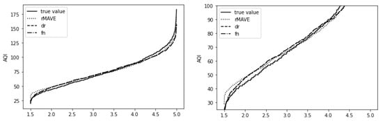
7. Conclusions

This work considers an estimation problem in single-index models with spatio-temporal correlation and heterogeneity. We propose a parametric component reweighting estimated method based on the variance function of the error. Theoretical results show that the proposed reweighting estimators have smaller asymptotic variances while maintaining the same biases. Numerical simulations show that the estimators revealed that heterogeneity is closer to the true value. A real data analysis was conducted to illustrate the proposed methods.

Author Contributions

Methodology, H.H.; Formal analysis, Z.Z.; Writing—original draft, H.W.; Writing—review & editing, C.H. All authors have read and agreed to the published version of the manuscript.

Funding

This research was supported by the National Social Science Fund of China under Grant No. 22BTJ021.

Data Availability Statement

The data presented in this study are available on request from the corresponding author.

Conflicts of Interest

The authors declare no conflict of interest.

Appendix A. Assumptions

In order to obtain asymptotic results, we will assume throughout the paper that at any fixed moment t , { ε i , t , i I n } satisfies the following mixing condition: there exists a function φ 1 ( t ) 0 as t , φ 1 ( 0 ) = 1 , such that whenever E , E I n with finite cardinals
α ( β ( E ) , β ( E ) ) = sup { P ( A B ) P ( A ) P ( B ) | A β ( E ) , B β ( E ) } ψ 1 ( c a r d ( E ) , c a r d ( E ) ) φ 1 ( d ( E , E ) ) ,
where β ( E ) (resp, β ( E ) ) denotes the Borel σ —field generated by { ε i , t } i E (resp, { ε i , t } i E ), Card E (resp, Card E ) is the cardinality of E(resp, E ) and d ( E , E ) is the ordinary Euclidean distance. ψ 1 : N 2 R + is a symmetric positive function that is nondecreasing in each variable.
Similarly, we assume that at any fixed location i 0 ,   { ε i 0 , t , t T n } satisfies the following mixing condition: there exists a function φ 2 ( t ) 0 as t , φ 2 ( 0 ) = 1 , such that whenever G , G T n with finite cardinals
α ( β ( G ) , β ( G ) ) = sup { P ( A B ) P ( A ) P ( B ) | A β ( G ) , B β ( G ) } ψ 2 ( c a r d ( G ) , c a r d ( G ) φ 2 ( d ( G , G ) ) ,
where β ( G ) (resp, β ( G ) ) denote the Borel σ —field generated by { ε i 0 , t } t G (resp, { ε i 0 , t } t G ), ψ 2 : N 2 R + is a symmetric positive function that is nondecreasing in each variable. Furthermore, the random field { ( X i , t , Y i , t ) , i I n , t T n } also satisfies the above assumption.
The following conditions are imposed to obtain the asymptotic properties of the resulting estimators. They are not the weakest, but they are introduced to make the evidence easier.
(C1)
The density function f β ( v ) of β T X and its derivatives up to the third order are bounded on R for all β : β β 0   < δ where δ > 0 is a constant, E X 6 < , and E | Y | 3 < .
(C2)
The conditional mean g β ( v ) = E ( Y | β T X = v ) and its derivatives up to the third order are bounded for all β : β β 0   < δ where δ > 0 .
(C3)
K ( · ) is a symmetric univariate density function with finite moments of all orders and a bounded derivative. Bandwidth h n n 1 / 5 and lim n log ( 1 / h n ) / n h n 2 = 0 .
(C4)
L ( · ) is a symmetric multivariate density function with finite moments and bounded derivatives. Bandwidth l n n d / 5 and lim n log ( 1 / l n d ) / n l n 2 d = 0 . s > 2 , δ ˜ < 1 s 1 , such that lim n n 2 δ ˜ 1 l n = + .
(C5)
Q ( · ) is a symmetric univariate density function with finite moments and bounded derivatives. Bandwidth b n n 1 / 5 and lim n log ( 1 / b n ) / n b n 2 = 0 . s > 2 , ρ ˜ < 1 s 1 , such that lim n n 2 ρ ˜ 1 b n = + .
According to (C1), covariate X can have discrete components provided that β T X is continuous for β in a small neighbor of β 0 ; see also [23]. In order to be able to use the optimal bandwidth, there needs to be a moment of order higher than the second order moment for the variable Y. The smoothness requirement of the link function in hypothesis (C2) can be relaxed to the existence of a bounded second-order derivative but requires a more complex proof process and a smaller bandwidth. The hypotheses (C3)–(C5) are common hypotheses in kernel regression; see [13].
Let ξ n = ( n h n / log n ) 1 / 4 , κ n = h n 2 + ξ n , and δ β = β β 0 . For any k, e k denotes a k-dimension vector with all elements equal to 1, and E k denotes a p × p matrix with all elements equal to 1. For any vector V ( v ) of functions of v, we define ( V ( v ) ) = d V ( v ) / d v . Recall that K ( · ) is a symmetric density function. Thus, μ 0 = K ( v ) d v = 1 and μ 1 = v K ( v ) d v = 0 . For ease of exposition, we assume that μ 2 = v 2 K ( v ) d v = 1 . Otherwise, K ( v ) = μ 2 1 / 2 K ( μ 2 1 / 2 v ) . Let D n = { x   :   x   <   n c , f β ( β T x ) > n ϵ , β B n } , where B n = { β   :   β β 0   <   n 1 + 2 c 0 } , c 1 . In order to prove the result of the theorems, we first present the following lemmas.

Appendix B. Proof

Lemma A1. 
Suppose m n ( χ , Z ) , n = 1 , 2 , , are measurable functions of Z with index χ R d , where d is any integer number, such that ( i )   | m n ( χ , Z ) | a n M ( Z ) with E ( M ( Z ) r ) < for some r > 2 , and a n increases with n such that a n < c 0 n 1 2 / r ; ( i i )   E ( m n ( χ , Z ) ) a n m 0 2 ( χ ) with | m 0 ( χ ) m 0 ( χ ) |   c χ χ α 1 , where α 1 > 0 and c > 0 are two constants (without loss of generality, we assume m 0 ( χ ) 1 ); and that ( i i i )   | m n ( χ , Z ) m n ( χ , Z ) |     | χ χ | α 1 n α 2 G ( Z ) with some α 2 > 0 , and E G 2 ( Z ) exists. Suppose { Z i , i = 1 , , n } is a random sample from Z. Then, for any positive α 0 , we have:
sup | χ | n α 0 | { m 0 ( χ ) } 1 n 1 i I n t T n { m n ( χ , Z i , t ) E m n ( χ , Z i , t ) } | = O P { ( a n log n / n ) 1 / 4 } .
Proof of Lemma A1. 
For the “continuity argument” approach, see [13,25]. For simplicity, let m n ( χ , Z ) denote m n ( χ , Z ) / m 0 ( χ ) . Let D n = def | χ | < n α 0 be bounded and its Borel measure be less than n d + α 0 . There are n α 4 ( α 4 > d + α 0 ) balls B n k centered at χ n k , 1 k n α 4 with a diameter smaller than c n 2 ( 2 + α 2 ) / α 1 , so that D n 1 k n α 4 B n k . Then,
s u p χ D n 1 n i I n t T n m n χ , Z i , t E m n χ , Z i , t m a x 1 k n α 4 1 n i I n t T n m n χ n k , Z i , t E m n χ n k , Z i , t + max 1 k n α 4 sup χ B n k 1 n i I n t T n m n χ , Z i , t m n χ n k , Z i , t E m n χ , Z i , t m n χ n k , Z i , t = def m a x 1 k n α 4 R n , k , 1 + m a x 1 k n α 4 s u p χ B n k R n , 2 .
By ( i i ) , we have:
m a x 1 k n α + s u p χ B n k m χ , Z i , t m χ n k , Z i , t m a x 1 k n α + s u p χ B n k n α 2 χ χ n k α 1 G Z i , t c n 2 G Z i , t .
By assumption ( i i i ) ,
m a x 1 k n α + s u p χ B n k R n , 2 c n 2 i I n t T n G Z i , t = O n 1 .
Let L n = n l o g ( n ) a n 8 9 , m n L χ , Z i , t = m n χ n k , Z i , t I M Z i , t L n , and m n O χ , Z i , t = m n χ n k , Z i , t m n L χ , Z i , t ; then, we have:
R n , k , 1 = 1 n i I n t T n m n L χ n k , Z i , t E m n L χ n k , Z i , t + 1 n i I n t T n ξ n k , i , t ,
where ξ n k , i , t = m n O χ n k , Z i , t E m n O χ n k , Z i , t . Because of P ( | M ( Z ) | > L n ) L n r E | M ( Z ) | r and n = 1 T n r < , for all sufficiently large n , with probability 1, | M ( Z i , t ) | L n for ( i , t ) . This implies that the first term on the right-hand side of (A5) is eventually 0. By assumption ( i i ) , we have:
m a x 1 k n α 4 Var i I n t T n n ξ n k , i , t c 1 n a n = def S 1 .
By ( i ) , we can obtain:
m a x 1 k n α ξ n k , i , t c 0 a n T n c n a n log n 1 / 9 = def S 2 .
Let S 3 = c n a n log n 3 4 , N = S 3 c S 2 . According to Theorem 2.1 of [26],
P i I n t T n ξ n k , i , t > S 3 4 exp S 3 2 64 n N S 1 + 8 3 S 3 N S 2 1 + 4 n N α N exp c a n log n n 1 8 + 4 n N α N .
According to the α mixing condition, α N 0 when N is large enough. Hence,
n = 1 Pr max 1 k n α 4 i I n t T n ξ n k , i , t S 3 < .
By the Borel-Cantelli lemma, we have:
max 1 k n α 4 i I n t T n ξ n k , i , t = O S 3 .
Combining (A4) and (A9), we have:
max 1 k n α 4 R n , k , 1 = O ( S 3 ) .
Therefore, Lemma A1 follows. □
Lemma A2 ([11]). 
Assume that φ ( β ) and ϕ ( β ) are two measurable functions of ( X , Y ) such that sup β , θ | φ ( β ) φ ( θ ) | < | β θ | ζ a . s . , sup β , θ | ϕ ( β ) ϕ ( θ ) | < | β θ | ζ a . s . , with E ζ r < c for some r > 2 , and E { ϕ ( β ) | β T X } = 0 for all β B . Suppose that ( X i , t , Y i , t ) , φ i ( β ) , and ϕ i ( β ) , i = 1 , , n are random copies of ( X , Y ) , φ ( β ) and ϕ ( β ) , respectively. If (C1), (C3), and (C4) hold, then:
sup β B 1 2 i = 1 n j = 1 n [ K h n ( β T X i j ) φ j ( β ) E j { K h n ( β T X i j ) φ j ( β ) } ] ϕ i ( β ) = O ( ξ n 2 ) .
Lemma A3. 
Suppose E ( Z | β T X = β T x ) = m ( β T x ) and its derivatives up to the second order are bounded for all β B , and suppose that E Z r exists for some r > 3 . Let ( X i , t , Z i , t ) be a sample from ( X , Z ) and X ( i , t ) x = X i , t x . If conditions (C1), (C3), and (C4) hold, then:
n 1 i I n t T n K h n ( β T X ( i , t ) x ) ( β T X ( i , t ) x / h n ) p Z i = f β ( β T x ) m ( β T x ) μ p + { f β ( β T x ) m ( β T x ) } μ p + 1 h n + O P ( κ n ) ,
where μ p = K ( v ) v p d v , p = 0 , 1 , .
Proof of Lemma A3. 
Since:
E { K h n ( β T X ( i , t ) x ) ( β T X ( i , t ) x / h n ) p m ( β T X i , t ) } = f β ( β T x ) m ( β T x ) μ p + { f β ( β T x ) m ( β T x ) } μ p + 1 h n + O P ( h n 2 ) ,
where μ p = v p K ( v ) d v , combining it with Lemma A1, we complete the proof of Lemma A3. □
Lemma A4. 
Let
Σ n β ( x ) = n 1 i I n t T n K h n ( β T X ( i , t ) x ) 1 β T X ( i , t ) x / h n 1 β T X ( i , t ) x / h n T ,
and
a x β b x β h n = { n Σ n β ( x ) } 1 i = 1 n K h n ( β T X ( i , t ) x ) 1 β T X ( i , t ) x / h n Y i , t .
Under conditions (C1)–(C4), we have:
a x β = g ( β 0 T x ) + g ( β 0 T x ) v β 0 T ( x ) ( β 0 β ) + 1 2 g ( β 0 T x ) h n 2 + Θ n , 1 ( x ) + O P { ( h n κ n + δ β 2 ) n ϵ } ( 1 + x 4 ) ,
b x β h n = g ( β 0 T x ) h n + Θ n , 2 ( x ) + O P { ( h n κ n + δ β 2 ) n ϵ e p } ( 1 + x 4 ) ,
where:
Θ n , 1 ( x ) = { n f β ( β T x ) } 1 i I n t T n K h n ( β T X ( i , t ) x ) ε i , t ,
and
Θ n , 2 ( x ) = { n h n f β ( β T x ) } 1 i I n t T n K h n ( β T X ( i , t ) x ) β T X ( i , t ) x ε i , t .
Proof of Lemma A4. 
By the Taylor expansion of g ( β 0 T X i , t ) at β 0 T x and β 0 = β + ( β 0 β ) , we have:
Y i , t = g ( β 0 T x ) + g ( β 0 T x ) β 0 T + 1 2 g ( β 0 T x ) ( β 0 T X ( i , t ) x ) 2 + ε i , t + O ( | β 0 T X ( i , t ) x | 3 ) = g ( β 0 T x ) + g ( β 0 T x ) β 0 T X ( i , t ) x + 1 2 g ( β 0 T x ) ( β 0 T X ( i , t ) x ) 2 + ε i , t + Ω n ( x , X i , t , β ) = g ( β 0 T x ) + g ( β 0 T x ) β T X ( i , t ) , x + 1 2 g ( β 0 T x ) ( β 0 T X ( i , t ) , x ) 2 + g ( β 0 T x ) ( β 0 β ) T X ( i , t ) , x + ε i , t + Ω n ( x , X i , t , β ) ,
where Ω n ( x , X i , β ) = O ( | β T X ( i , t ) , x | 3 + | β T X ( i , t ) , x | · X ( i , t ) , x δ β + X ( i , t ) , x 2 δ β 2 ) . By Equation (A11), it follows that:
a x β b x β h n = { n Σ n β ( x ) } 1 i I n t T n K h n ( β T X ( i , t ) , x ) 1 β T X ( i , t ) , x / h n · { g ( β 0 T x ) + g ( β 0 T x ) β T X ( i , t ) , x } + { n Σ n β ( x ) } 1 i I n t T n K h n ( β T X ( i , t ) , x ) 1 β T X ( i , t ) , x / h n 1 2 g ( β 0 T x ) ( β 0 T X ( i , t ) , x ) 2 + { n Σ n β ( x ) } 1 i I n t T n K h n ( β T X ( i , t ) , x ) 1 β T X ( i , t ) , x / h n g ( β 0 T x ) ( β 0 β ) T X ( i , t ) , x + { n Σ n β ( x ) } 1 i I n t T n K h n ( β T X ( i , t ) , x ) 1 β T X ( i , t ) , x / h n ε i , t + { n Σ n β ( x ) } 1 i I n t T n K h n ( β T X ( i , t ) , x ) 1 β T X ( i , t ) , x / h n Ω n ( x , X i , t , β ) : = A 1 + A 2 + A 3 + A 4 + A 5 .
According to Lemma A3, we have:
Σ n β ( x ) = f β ( β T x ) f β ( β T x ) h n f β ( β T x ) h n f β ( β T x ) + O p ( κ n ) .
If f β ( β T x ) > n ϵ , we have:
{ Σ n β ( x ) } 1 = f β 1 ( β T x ) I f β 1 0 f β ( β T x ) h n f β ( β T x ) h n 0 + O p ( κ n n ϵ ) .
It is easy to check that
A 1 = g ( β 0 T x ) g ( β 0 T x ) h n .
According to Lemma A3 and Equation (A11), we have:
A 2 = g ( β 0 T x ) h n 2 g ( β 0 T x ) f β ( β T x ) h n 3 + O p ( h n κ n n ϵ e d + 1 ) .
By Lemma A3, we have:
A 3 = g ( β 0 T x ) v β T ( x ) ( β 0 β ) O ( h n δ β ) ( 1 + x ) + O p ( κ n δ β n ϵ e d + 1 ) ( 1 + x ) .
For the noise term, we have:
A 4 = { n f β ( β T x ) } 1 i = 1 n K h n ( β T X ( i , t ) , x ) 1 β T X ( i , t ) , x / h n ε i , t + O p ( κ n δ β n ϵ e d + 1 ) .
It follows from Lemma A2 that:
n 1 i = 1 n K h n ( β T X ( i , t ) , x ) 1 β T X ( i , t ) , x / h n | β T X ( i , t ) , x | k X ( i , t ) , x l = O p ( h n k ) ( 1 + x l ) .
Then, we have:
A 5 = O p { ( h n 3 + δ β 2 ) n ϵ e d + 1 } ( 1 + x 3 ) .
Thus, Lemma A4 follows from (A13)–(A17). □
Lemma A5. 
Under conditions (C1)–(C4), we have:
n 2 j I n τ T n i I n t T n ρ ^ j , τ β ( b j , τ β ) 2 K h n ( β T X ( i , t ) , ( j , τ ) ) X ( i , t ) , ( j , τ ) X ( i , t ) , ( j , τ ) T / f ^ β ( β T X j , τ ) 1 = β 0 β 0 T [ E { g ( β 0 T X ) 2 } ] 1 h n 2 1 2 [ E { g ( β 0 T X ) 2 } ] 1 ( β 0 F T W g 0 + + W g 0 + F β 0 T ) + 1 2 W g 0 + + O P { ( κ n h n n ϵ + δ β / h n 2 ) E d } ,
where W g 0 = E { g ( β 0 T X ) 2 v β 0 ( X ) v β 0 T ( X ) } and F = E { [ g ( β 0 T X ) ] 2 ( f β 0 ( β 0 T X ) v β 0 ( X ) ) f β 0 ( β 0 T X ) } .
Proof of Lemma A5. 
According to condition (C1), we have:
i I n t T n P ( i I n t T n { X i , t D n } ) i I n t T n n P ( X i , t D n ) i I n t T n n P ( | X i , t | n c ) < i I n t T n n n 6 c E | X | 6 < .
By the Borel–Cantelli lemma, we have:
P i I n t T n { X i , t D n } , i . o . = 0 .
Let D ˜ n = { x : f β ( β T x ) > 2 n ϵ } . Similarly, we have:
P i I n t T n { X i , t D ˜ n } , i . o . = 0 .
Hence, we can exchange summations over { X j , τ : j I n , τ T n } , { X j , τ : X j , τ D n , j I n , τ T n } , { X j , τ : X j , τ D ˜ n , j I n , τ T n } in the sense of almost sure consistently. By Lemma A3 and condition (C1), we have:
f ^ β ( β T x ) = f β ( β T x ) + O ( κ n ) .
By Equation (A19) and the smoothness of ρ n ( · ) with | ρ n ( · ) | < c n ϵ for some c > 0 , we have:
ρ n ( f ^ β ( β T x ) ) = ρ n ( f β ( β T x ) ) + O ( κ n n ϵ ) = 1 + O ( κ n n ϵ ) .
Denote by ( β , D ) an orthogonal matrix. According to Lemma A3, we have:
n 1 i I n t T n K h n ( β T X ( i , t ) , x ) β T X ( i , t ) , x X ( i , t ) , x T β = f β ( β T x ) h n 2 + O p ( h n 2 κ n ) , n 1 i I n t T n K h n ( β T X ( i , t ) , x ) β T X ( i , t ) , x X ( i , t ) , x T D = f β ( β T x ) v β T ( x ) D h n 2 + O p ( h n 2 κ n e p 1 ) , n 1 i I n t T n K h n ( β T X ( i , t ) , x ) D T X ( i , t ) , x X ( i , t ) , x T D = f β ( β T x ) C β ( x ) + O p ( κ n E p 1 ) ( 1 + | x | 2 ) ,
where C β ( x ) = D T w ˜ β ( x ) D , w ˜ β ( x ) = w β ( x ) x μ β T ( x ) μ β ( x ) x T + x x T . It follows from (A19) that:
{ n f ^ β ( β T x ) } 1 i I n t T n K h n ( β T X ( i , t ) , x ) X ( i , t ) , x X ( i , t ) , x T = ( β , D ) h n 2 F β T ( x ) D h n 2 D T F β ( x ) h n 2 C β ( x ) ( β , D ) T + O p ( h n κ n n ϵ E d ) ( 1 + x 2 ) ,
where F β ( x ) = f β ( β T x ) v β ( x ) / f β ( β T x ) . According to (A20), we have: b x β = g ( β 0 T x ) + O ( κ n n 2 ϵ / h n ) ( 1 + x 4 ) . Note that E { g ( β 0 T X j , τ ) 2 C β 0 ( X j , τ ) } = 2 D 0 T W g 0 D 0 . Thus,
n 2 i I n t T n j I n τ T n ρ ^ j , τ β ( b j , τ β ) 2 K h n ( β T X ( i , t ) , ( j , τ ) ) X ( i , t ) , ( j , τ ) X ( i , t ) , ( j , τ ) T / f ^ β ( β T X j , τ ) = n 1 X j , τ D n ρ n ( f ^ β ( β T X j , τ ) ) ( b j , τ β ) 2 { n f ^ β ( β T X j , τ ) } 1 · i I n t T n K h n ( β T X ( i , t ) , x ) X ( i , t ) , ( j , τ ) X ( i , t ) , ( j , τ ) T = ( β , D ) n 1 j I n τ T n g ( β 0 T X j , τ ) 2 h n 2 F β T ( X j , τ ) D h n 2 D T F β ( X j τ ) h n 2 C β ( X j , τ ) + O ( h n κ n n ϵ ) ( 1 + | X j , τ | 6 ) ( β , D ) T = ( β , D ) E { g ( β 0 T X ) 2 } h n 2 F T D h n 2 D T F h n 2 2 D T W g 0 D ( β , D ) T + O ( h n κ n n ϵ + δ β E d ) ,
where F = E { [ g ( β 0 T X ) ] 2 F β 0 ( X ) } . Therefore, by the matrix inversion formula in blocks [27], we have:
n 2 i I n t T n j I n τ T n ρ ^ j , τ β ( b j , τ β ) 2 K h n ( β T X ( i , t ) , ( j , τ ) ) X ( i , t ) , ( j , τ ) X ( i , t ) , ( j , τ ) T / f ^ β ( β T X j ) 1 = β β T [ E { g ( β 0 T X j , τ ) 2 } ] 1 h n 2 1 2 [ E { g ( β 0 T X j , τ ) 2 } ] 1 ( D H D T F β T + β F T D T H D ) + 1 2 D H D T + O { h n 2 ( h n κ n n ϵ + δ β ) E d } ,
where H = ( D T W g 0 D ) 1 . Note that D = D 0 + δ β . Then, H = ( D 0 T W g 0 D 0 ) 1 + δ β . By the definition of the Moore–Penrose inverse, we have:
D 0 ( D 0 T W g 0 D 0 ) 1 D 0 T = W g 0 + .
Combining the facts that D D T = I β β T = I β 0 β 0 T + O ( δ β ) and β 0 T W g 0 = 0 , we complete the proof. □
Lemma A6. 
Under conditions (C1)–(C4), we have:
n 2 j I n τ T n i I n t T n ρ ^ j , τ β K h n ( β T X ( i , t ) , ( j , τ ) ) b j , τ β X ( i , t ) , ( j , τ ) ( Y i , t a j , τ β b j , τ β β 0 T X ( i , t ) , ( j , τ ) ) ) / f ^ β ( β T X j , τ ) = W g 0 ( β β 0 ) + n 1 i I n t T n g ( β 0 T X i , t ) v β 0 ( X i , t ) ε i , t + o P ( n 1 / 2 e d ) .
Proof of Lemma A6. 
According to Lemma A4, we have:
n 2 j I n τ T n i I n t T n ρ ^ j , τ β K h n ( β T X ( i , t ) , ( j , τ ) ) b j , τ β X ( i , t ) , ( j , τ ) ( Y i a j , τ β b j , τ β β 0 T X ( i , t ) , ( j , τ ) ) / f ^ β ( β T X j , τ ) = n 2 j I n τ T n i I n t T n ρ ^ j , τ β f ^ β 1 ( β T X j , τ ) K h n ( β T X ( i , t ) , ( j , τ ) ) b j , τ β X ( i , t ) , ( j , τ ) ε i , t + n 2 j I n τ T n i I n t T n ρ ^ j , τ β f ^ β 1 ( β T X j , τ ) K h n ( β T X ( i , t ) , ( j , τ ) ) b j , τ β X ( i , t ) , ( j , τ ) g ( β 0 T X j , τ ) v β T ( X j , τ ) ( β β 0 ) + n 2 j I n τ T n i I n t T n ρ ^ j , τ β f ^ β 1 ( β T X j , τ ) K h n ( β T X ( i , t ) , ( j , τ ) ) b j , τ β X ( i , t ) , ( j , τ ) 1 2 g ( β 0 T X j , τ ) × { ( β T X ( i , t ) , ( j , τ ) ) 2 h n 2 } n 2 j I n τ T n i I n t T n ρ ^ j , τ β f ^ β 1 ( β T X j , τ ) K h n ( β T X ( i , t ) , ( j , τ ) ) × b j , τ β X ( i , t ) , ( j , τ ) { Θ n , 1 ( X j , τ ) + Θ n , 2 ( X j , τ ) β 0 T X ( i , t ) , ( j , τ ) / h n } + n 2 j I n τ T n i I n t T n ρ ^ j , τ β f ^ β 1 ( β T X j , τ ) K h n ( β T X ( i , t ) , ( j , τ ) ) b j , τ β X ( i , t ) , ( j , τ ) × O { ( h n κ n + δ β 2 ) n ϵ } ( 1 + | X j , τ | 4 ) ( 1 + | β 0 T X ( i , t ) , ( j , τ ) | / h n ) : = B 1 + B 2 + B 3 + B 4 + B 5 .
Denote by U ( i , t ) , ( j , τ ) = ρ n ( f β ( β T X j , τ ) ) K h n ( β T X ( i , t ) , ( j , τ ) ) b j , τ β X ( i , t ) , ( j , τ ) . We have E { E j , τ ( U ( i , t ) , ( j , τ ) ) g ( β 0 T X j , τ ) v β ( X j , τ ) } 2 = O { ( h n + δ β ) 2 } . Note that Θ n , 1 = O ( κ n n ϵ ) and Θ n , 2 = O ( κ n n ϵ ) . By Lemmas A1 and A2, we have:
B 1 = n 2 j I n τ T n i I n t T n { U ( i , t ) , ( j , τ ) E j ( U ( i , t ) , ( j , τ ) ) } ε i , t + n 1 i I n t T n E j ( U ( i , t ) , ( j , τ ) ) ε i , t + o d ( n 1 / 2 e d ) = n 1 i I n t T n g ( β 0 T X i , t ) v β ( X i , t ) ε i + o p ( n 1 / 2 e d ) .
According to Lemma A3, (A18) and (A19), we have:
B 2 = W g 0 ( β β 0 ) + O p { ( κ n + δ β ) e d / h n } .
By Lemmas A3 and A4, we have:
B 3 = O p { ( h n 2 κ n n ϵ e d } .
Letting V ( i , t ) , ( j , τ ) = K h n ( β T X ( i , t ) , ( j , τ ) ) X ( i , t ) , ( j , τ ) , then we have E i ( V ( i , t ) , ( j , τ ) ) = v β ( X j , τ ) + O p ( h n 2 e d ) ( 1 + X j , τ ) . Note that E { v β ( X j , τ ) } = 0 . According to Lemma A2, we have:
B 4 = n 2 j I n τ T n i I n t T n ρ n ( f β ( β T X j , τ ) ) V ( i , t ) , ( j , τ ) g ( β T X j , τ ) f β 1 ( β T X j , τ ) × { Θ n , 1 ( X j , τ ) + Θ n , 2 ( X j , τ ) β 0 T X ( i , t ) ( j , τ ) / h n } + O p ( n 1 / 2 e d ) = n 1 j I n τ T n ρ n ( f β ( β T X j , τ ) ) v β ( X j , τ ) g ( β T X j , τ ) f β 1 ( β T X j , τ ) × { Θ n , 1 ( X j , τ ) + Θ n , 2 ( X j , τ ) β 0 T X ( i , t ) , ( j , τ ) / h n } + O p ( n 1 / 2 e d ) = O p ( n 1 / 2 ) e d .
By Lemma A1 and Corollary 2 in [28] ( p. 122), we have:
B 5 = O p { ( h n κ n + δ β 2 e d ) n ϵ } O ( 1 ) n 1 j I n τ T n | X j , τ | 5 = O p { ( h n κ n + δ β 2 ) n ϵ e d } .
Combining (A21)–(A25), we complete the proof of this lemma. □
Lemma A7. 
According to Theorem 3 in [29], for δ < 1 s 1 lim n + n 2 δ 1 h ˜ = + , we have:
sup x R d | 1 n i I n t T n K ˜ h ˜ ( X ˜ i , t x ) Y ˜ i , t E ( K ˜ h ˜ ( X ˜ i , t x ) Y ˜ i , t ) | = O p ( l o g ( n ) n h ˜ d ) .
Lemma A8. 
Under conditions (C1)–(C5), we have:
sup x R d σ β 0 2 ( x ) i I n t T n w ˜ i , t ( x ) σ β 0 2 ( x ) = O p h ˜ 2 d + l o g ( 1 / h ˜ d ) n h ˜ d 1 2 ,
where:
w ˜ i , t ( x ) = K ˜ h ˜ ( X i , t x ) j I n τ T n K ˜ h ˜ ( X j , τ x ) , j I n , τ T n .
Proof of Theorem 1. 
For any x R d , let:
ϖ j , τ ( x ) = L l n ( X j , τ x ) i I n t T n L l n ( X i , t x ) .
According to Equations (9) and (10), by Lemma A4, we have:
σ ^ β ^ n 2 ( x ) j I n τ T n ε ^ j , τ 2 ϖ j , τ ( x ) = j I n τ T n ( Y j , τ a i , t β ^ n ) 2 ϖ j , τ ( x ) = j I n τ T n Y j , τ g ( β 0 T X j , τ ) g ( β 0 T X j , τ ) v β 0 T ( X j , τ ) ( β 0 β ^ n ) 1 2 g ( β 0 T X j , τ ) h n 2 Θ n , 1 ( X j , τ ) 2 · ϖ j , τ ( x ) = j I n τ T n ε j , τ 2 ϖ j , τ ( x ) + j I n τ T n g ( β 0 T X j , τ ) 2 v β 0 T ( X j , τ ) ( β 0 β ^ n ) v β 0 T ( X j , τ ) ( β 0 β ^ n ) ϖ j , τ ( x ) + 1 4 j I n τ T n g ( β 0 T X j , τ ) 2 h n 4 ϖ j , τ ( x ) + j I n τ T n Θ n , 1 ( X j , τ ) 2 ϖ j , τ ( x ) 2 j I n τ T n g ( β 0 T X j , τ ) v β 0 T ( X j , τ ) ( β 0 β ^ n ) ε j , τ ϖ j , τ ( x ) j I n τ T n g ( β 0 T X j , τ ) h n 2 ε j , τ ϖ j , τ ( x ) 2 j I n τ T n Θ n , 1 ( X j , τ ) ε j , τ ϖ j , τ ( x ) + j I n τ T n g ( β 0 T X j , τ ) h n 2 Θ n , 1 ( X j , τ ) ϖ j , τ ( x ) + j I n τ T n g ( β 0 T X j , τ ) v β 0 T ( X j , τ ) ( β 0 β ^ n ) g ( β 0 T X j , τ ) h n 2 ϖ j , τ ( x ) + 2 j I n τ T n g ( β 0 T X j , τ ) v β 0 T ( X j , τ ) ( β 0 β ^ n ) Θ n , 1 ( X j , τ ) ϖ j , τ ( x ) : = C 1 + C 2 + C 3 + C 4 + C 5 + C 6 + C 7 + C 8 + C 9 + C 10 .
Thus, we can obtain from the results in Lemmas A7 and A8 that:
sup x R d C 1 σ β 0 2 ( x ) = sup x R d C 1 j I n τ T n ϖ j , τ ( x ) σ β 0 2 ( X j , τ ) + j I n τ T n ϖ j , τ ( x ) σ β 0 2 ( X j , τ ) σ β 0 2 ( x ) sup x R d C 1 j I n τ T n ϖ j , τ ( x ) σ β 0 2 ( X j , τ ) + sup x R d j I n τ T n ϖ j , τ ( x ) σ β 0 2 ( X j , τ ) σ β 0 2 ( x ) = O p l n 2 d + l o g ( 1 / l n d ) n l n d 1 2 .
Since β ^ n B n , applying the result of Lemma A7 obtains:
sup x R d | C 2 | = sup x R d j I n τ T n g ( β 0 T X j , τ ) 2 v β 0 T ( X j , τ ) ( β 0 β ^ n ) v β 0 T ( X j , τ ) ( β 0 β ^ n ) ϖ j , τ ( x ) = O p n 1 + 2 c 0 ,
sup x R d | C 3 | = sup x R d 1 4 j I n τ T n g ( β 0 T X j , τ ) 2 h n 4 ϖ j , τ ( x ) = O p h n 4 ,
sup x R d | C 4 | = sup x R d j I n τ T n Θ n , 1 ( X j , τ ) 2 ϖ j , τ ( x ) = O p l o g ( n ) n l n d ,
sup x R d | C 5 | = sup x R d 2 j I n τ T n g ( β 0 T X j , τ ) v β 0 T ( X j , τ ) ( β 0 β ^ n ) ε j , τ ϖ j , τ ( x ) = O p n 1 + 2 c 0 · l o g ( n ) n l n d 1 2 ,
sup x R d | C 6 | = sup x R d j I n τ T n g ( β 0 T X j , τ ) h n 2 ε j , τ ϖ j , τ ( x ) = O p ( h n 2 ) · O p l o g ( n ) n l n d 1 2 ,
sup x R d | C 7 | = sup x R d 2 j I n τ T n Θ n , 1 ( X j , τ ) ε j , τ ϖ j , τ ( x ) = O p l o g ( n ) n l n d ,
sup x R d | C 8 | = sup x R d j I n τ T n g ( β 0 T X j , τ ) h n 2 Θ n , 1 ( X j , τ ) ϖ j , τ ( x ) = O p ( h n 2 ) · O p l o g ( n ) n l n d 1 2 ,
sup x R d | C 9 | = sup x R d j I n τ T n g ( β 0 T X j , τ ) v β 0 T ( X j , τ ) ( β 0 β ^ n ) g ( β 0 T X j , τ ) h n 2 ϖ j , τ ( x ) = O p h n 2 · n 1 + 2 c 0 ,
sup x R d | C 10 | = sup x R d 2 j I n τ T n g ( β 0 T X j , τ ) v β 0 T ( X j , τ ) ( β 0 β ^ n ) Θ n , 1 ( X j , τ ) ϖ j , τ ( x ) = O p n 1 + 2 c 0 · O p l o g ( n ) n l n d 1 2 .
Thus, combining (A26)–(A36), we complete the proof of Theorem 1. □
Proof of Theorem 2. 
Theorem 2 can be proven in the same way as Theorem 1, so it is omitted here. □
Proof of Theorem 3. 
After one iteration, by Lemmas A5 and A6, we have that the new β ( 1 ) is:
β ( 1 ) = β 0 + j I n τ T n i I n t T n ρ ^ j , τ β ( b j , τ β ) 2 K h n ( β T X ( i , t ) , ( j , τ ) ) X ( i , t ) , ( j , τ ) X ( i , t ) , ( j , τ ) T / f ^ β ( β T X j , τ ) 1 × j I n τ T n i I n t T n ρ ^ j , τ β K h n ( β T X ( i , t ) , ( j , τ ) ) X ( i , t ) , ( j , τ ) ( Y i , t a j , τ β b j , τ β β 0 T X ( i , t ) , ( j , τ ) ) / f ^ β ( β T X j , τ ) = β 0 + h n 2 { E [ g ( β 0 T X ) ] 2 } 1 β 0 β 0 T W g 0 ( β β 0 ) + h n 2 { E [ g ( β 0 T X ) ] 2 } 1 1 n i = 1 n g ( β 0 T X i , t ) β 0 β 0 T v β 0 ( X i , t ) ε i , t 1 2 { E [ g ( β 0 T X ) ] 2 } 1 β 0 F T W g 0 + W g 0 ( β β 0 ) 1 2 n { E [ g ( β 0 T X ) ] 2 } 1 i I n t T n g ( β 0 T X i , t ) β 0 F T W g 0 + v β 0 ( X i , t ) ε i , t 1 2 { E [ g ( β 0 T X ) ] 2 } 1 W g 0 + F β 0 T W g 0 ( β β 0 ) 1 2 n { E [ g ( β 0 T X ) ] 2 } 1 i I n t T n g ( β 0 T X i , t ) W g 0 + F β 0 T v β 0 ( X i , t ) ε i , t + 1 2 W g 0 + W g 0 ( β β 0 ) + 1 2 n W g 0 + i I n t T n g ( β 0 T X i , t ) v β 0 ( X i , t ) ε i , t = β 0 + 1 2 ( I β 0 β 0 T ) ( β β 0 ) + 1 2 n W g 0 + i I n t T n g ( β 0 T X i , t ) v β 0 ( X i , t ) ε i , t + O p ( n 1 2 e d ) ;
the last equation holds because β 0 T v β 0 ( X i , t ) = 0 , β 0 T W g 0 = 0 , W g 0 + W g 0 = I β 0 β 0 T , and
1 2 n F T W g 0 + i I n t T n g ( β 0 T X i , t ) v β 0 ( X i , t ) ε i , t + 1 2 F T W g 0 + W g 0 ( β β 0 ) = O p ( e d ) .
It is easy to check that β ( 1 ) = 1 + o ( 1 ) , so then β ( 1 ) / β ( 1 ) = β ( 1 ) . Let β ( k ) be the value of β after k iterations. We have:
β ( k + 1 ) = β 0 + 1 2 ( I β 0 β 0 T ) ( β ( k ) β 0 ) + 1 2 n W g 0 + i I n t T n g ( β 0 T X i , t ) v β 0 ( X i , t ) ε i , t + + O p ( n 1 2 e d ) .
Recursing the preceding equation, we have, as the iteration k :
β ( k ) = β 0 + 1 2 k 1 ( I β 0 β 0 T ) ( β ( 1 ) β 0 ) + ( 1 1 2 k 1 ) 1 n W g 0 + i I n t T n g ( β 0 T X i , t ) v β 0 ( X i , t ) ε i , t β 0 + 1 n W g 0 + i I n t T n g ( β 0 T X i , t ) v β 0 ( X i , t ) ε i , t .
The following lemmas are used to prove Theorem 3. □
Lemma A9. 
(i) Suppose (A1) holds, and let L l 1 ( F ) denote the class of F —measurable r.v’s X satisfying X l 1 = ( E | X | l 1 ) 1 l 1 < . Let X L l 1 ( B ( E ) ) , Y L l 2 ( B ( E ) ) . Suppose 1 l 1 , l 2 , l 3 < , and l 1 1 + l 2 1 + l 3 1 = 1 ; then:
| E ( X Y ) E X E Y | c X l 1 Y l 2 { ψ 1 ( C a r d E , C a r d E ) φ 1 ( d ( E , E ) ) } 1 l 3 .
(ii) If, moreover, | X | and | Y | are P a . s bounded, the right-hand side of (A37) can be replaced with c ψ 1 ( C a r d E , C a r d E ) φ 1 ( d ( E , E ) ) .
Lemma A10. 
(i) Suppose (A2) holds, and let L l 1 ( F ) denote the class of F —measurable r.v’s X satisfying X l 1 = ( E | X | l 1 ) 1 l 1 < . Let X L l 1 ( B ( G ) ) , Y L l 2 ( B ( G ) ) . Suppose 1 l 1 , l 2 , l 3 < , a n d l 1 1 + l 2 1 + l 3 1 = 1 ; then:
| E ( X Y ) E X E Y | c X l 1 Y l 2 { ψ 2 ( C a r d G , C a r d G ) φ 2 ( d ( G , G ) ) } 1 l 3 .
(ii) If, moreover, | X | and | Y | are P a . s bounded, the right-hand side of (A38) can be replaced with c ψ 2 ( C a r d G , C a r d G ) φ 2 ( d ( G , G ) ) .
Lemma A11. 
Under assumptions (C1) and (C2), one has:
E n β ( k ) β 0 = 0 .
Proof of Lemma A11. 
E n β ( k ) β 0 = n E β 0 + 1 n W g 0 + i I n t T n g ( β 0 T X i , t ) v β 0 ( X i , t ) ε i , t β 0 = 1 n E W g 0 + i I n t T n g ( β 0 T X i , t ) v β 0 ( X i , t ) ε i , t = 0 .
Lemma A12. 
Under assumptions (C1)–(C5), one has:
V a r n β ( k ) β 0 = W g 0 + Δ W g 0 + ,
where W g 0 = E { g ( β 0 T X ) 2 W 0 ( X ) } and Δ = E { g ( β 0 T X ) 2 W 0 ( X ) σ β 0 2 ( X ) } .
Proof of Lemma A12. 
V a r n β ( k ) β 0 = 1 n i I n t T n V a r W g 0 + g ( β 0 T X i , t ) v β 0 ( X i , t ) ε i , t β 0 + 1 n i j t τ E W g 0 + g ( β 0 T X i , t ) v β 0 ( X i , t ) ε i , t W g 0 + g ( β 0 T X j , τ ) v β 0 ( X j , τ ) ε j , τ = J 1 + J 2 ,
J 1 = 1 n i I n t T n V a r W g 0 + g ( β 0 T X i , t ) v β 0 ( X i , t ) ε i , t = V a r W g 0 + g ( β 0 T X i , t ) v β 0 ( X i , t ) ε i , t β 0 = W g 0 + E { g ( β 0 T X ) 2 W 0 ( X ) σ β 0 2 ( X ) } W g 0 + .
By the boundedness of ( W g 0 + g ( β 0 T X i , t ) v β 0 ( X i , t ) for i I n , t T n , and then by the mixing condition, and similar to the proof of I 22 0 in Lemma 4.4 in [5],
J 2 = 1 n i j t τ E W g 0 + g ( β 0 T X i , t ) v β 0 ( X i , t ) ε i , t W g 0 + g ( β 0 T X j , τ ) v β 0 ( X j , τ ) ε j , τ c n i j t τ E ε i , t ε j , τ 0 .
Lemma A13. 
Under assumptions (C1)–(C5), one has:
n β ( k ) β 0 E n β ( k ) β 0 D N ( 0 , W g 0 + Δ W g 0 + ) .
Proof of Lemma A13. 
To simplify, let H n = W g 0 + g ( β 0 T X i , t ) v β 0 ( X i , t ) ε i , t , n β ( k ) β 0 E n β ( k ) β 0 = 1 n i I n t T n ( H n E H n ) . Then, let 1 n i I n t T n ( H n E H n ) = i I n t T n i , t .
Let us now introduce a space–time block decomposition, which has been used by [30]. Fix integers p k = O ( log n k ) 1 8 ( N + 1 ) , k = 1 , , N + 1 , q = O ( log n N + 1 ) 1 16 ( N + 1 ) , k = 1 , , N + 1 , and assume that, for some integer r,
n k = r ( p k + q ) a n d w e h a v e lim n p k q = , k = 1 , , N + 1 .
The random variables i , t are now set into blocks of different sizes. Let:
U ( 1 , n , j ) = i k = j k ( p k + q ) + 1 k = 1 , , N j k ( p k + q ) + p k t = j N + 1 ( p N + 1 + q ) + 1 j N + 1 ( p N + 1 + q ) + p N + 1 i , t , U ( 2 , n , j ) = i k = j k ( p k + q ) + 1 k = 1 , , N j k ( p k + q ) + p k t = j N + 1 ( p N + 1 + q ) + p N + 1 + 1 ( j N + 1 + 1 ) ( p N + 1 + q ) i , t , U ( 3 , n , j ) = i k = j k ( p k + q ) + 1 k = 1 , , N 1 j k ( p k + q ) + p k i N = j N ( p N + q ) + p N + 1 ( j N + 1 ) ( p N + 1 + q ) t = j N + 1 ( p N + 1 + q ) + 1 j N + 1 ( p N + 1 + q ) + p N + 1 i , t , U ( 4 , n , j ) = i k = j k ( p k + q ) + 1 k = 1 , , N 1 j k ( p k + q ) + p k i N = j N ( p N + q ) + p N + 1 ( j N + 1 ) ( p N + q ) t = j N + 1 ( p N + 1 + q ) + p N + 1 + 1 ( j N + 1 + 1 ) ( p N + 1 + q ) i , t ,
and so on. Note that:
U ( 2 N + 1 1 , n , j ) = i k = j k ( p k + q ) + p k + 1 k = 1 , , N ( j k + 1 ) ( p k + q ) t = j N + 1 ( p N + 1 + q ) + 1 j N + 1 ( p N + 1 + q ) + p N + 1 i , t .
Finally,
U ( 2 N + 1 , n , j ) = i k = j k ( p k + q ) + p k + 1 k = 1 , , N ( j k + 1 ) ( p k + q ) t = j N + 1 ( p N + 1 + q ) + p N + 1 + 1 ( j N + 1 + 1 ) ( p N + 1 + q ) i , t .
Setting R = { 0 , , r 1 } × × { 0 , , r 1 } , we define for each integer i = 1 , , 2 N + 1 ,
T ( n , i ) = j R U ( i , n , j ) .
Then, with this notation, we obtain the decomposition
1 n i I n t T n ( H n E H n ) = i = 1 2 N + 1 T ( n , i ) .
Note that T ( n , 1 ) is the sum of the random variables i , t over “large” blocks, whereas T ( n , i ) , 2 i 2 N + 1 are sums over “small” blocks. If it is not the case that n k = r ( p k + q ) for r, then an additional term T ( n , 2 N + 1 + 1 ) , say, containing all the i , t terms that are not included in the big or small blocks, can be considered. This term will not change the proof much.
The main idea is to show that, as n :
Q 1 = | E exp [ i u T ( n , 1 ) ] j k = 0 k = 1 , , N + 1 r 1 E exp [ i u U ( 1 , n , j ) ] | 0 ,
Q 2 = ( i = 2 2 N + 1 T ( n , i ) ) 2 0 ,
Q 3 = j k = 0 k = 1 , , N + 1 r 1 E [ U ( 1 , n , j ) ] 2 W g 0 + Δ W g 0 + ,
Q 4 = j k = 0 k = 1 , , N + 1 r 1 E [ ( U ( 1 , n , j ) ) 2 I { | U ( 1 , n , j ) | > ε W g 0 + Δ W g 0 + } ] 0 .
Proof of (A42)). 
The proof is similar to the proof of (5.42) in [31]. □
Proof of (A43). 
According to assumption (C1), if for each 2 i 2 N + 1 , E ( T ( n , i ) ) 2 0 exists, (A43) can be proven. Without loss of generality, it suffices to prove that, for E [ T ( n , 2 ) ] 2 0 . Enumerate the r.v’s U ( 2 , n , j ) in an arbitrary manner and refer to them as U ^ 1 , , U ^ M , where M = r N + 1 = ( n 1 p 1 + q ) ( n N + 1 p N + 1 + q ) . □
Now,
E [ T ( n , 2 ) ] 2 = j = 1 M V a r ( U ^ i ) + 2 i = 1 i M j = 1 j M C o v ( U ^ i , U ^ j ) = I 1 + I 2 .
If I 1 0 , and I 2 0 can be shown, Q 2 0 is obvious.
V a r i , t = V a r ( 1 n ( H n E H n ) ) = 1 n E ( H n E H n ) 2 = 1 n E W g 0 + E { g ( β 0 T X ) 2 W 0 ( X ) σ β 0 2 ( X ) } W g 0 +
c n .
Similar to (A47), we have:
E i , t j , τ = 1 n E W g 0 + g ( β 0 T X i , t ) v β 0 ( X i , t ) ε i , t W g 0 + g ( β 0 T X j , τ ) v β 0 ( X j , τ ) ε j , τ
c 1 n φ ( i j , | t τ | ) δ 2 + δ .
Then, by Equations (A47) and (A49), we have:
V a r ( U ^ i ) = V a r ( i k = 1 k = 1 , , N p k t = 1 q i , t ) i k = 1 k 1 , , N p k t = 1 q V a r i , t + j k = 1 k = 1 , , N i k j k f o r p k τ = 1 s o m e q i k = 1 k = 1 , , N 1 k N o r p k t = 1 t τ q | E j , τ i , t | i k = 1 k = 1 , , N p k t = 1 q V a r i , t + i k = 1 k = 1 , , N p k t = 1 t q τ = 1 τ q | E i , τ i , t | + i k = 1 f o r s o m e p k j k i k k = 1 , , N p k t = 1 t q τ = 1 τ q | E j , τ i , t | + t = 1 q i k = 1 f o r s o m e p k j k i k k = 1 , , N p k | E j , t i , t | .
By Lemma A9, the above inequality continues as:
c p 1 p N q n + c p 1 p N q n [ t = 1 φ 2 ( t ) δ 2 + δ + i k = 1 k = 1 , , N φ 1 ( i ) ) + q i k = 1 k = 1 , , N φ 1 ( i ) ] c p 1 p N q n [ 1 + t = 1 φ 2 ( t ) δ 2 + δ + q i = 1 i N φ 1 ( i ) δ 2 + δ ] c p 1 p N q 2 n .
Consequently,
I 1 M c p 1 p N q 2 n * = n * ( p 1 + q ) ( p N + 1 + q ) · c p 1 p N q 2 n * q 2 p N + 1 ,
which tends to zero by the definition of p k = O ( log n k ) 1 8 ( N + 1 ) and q = O ( log n N + 1 ) 1 16 ( N + 1 ) .
Let:
I ( 2 , n , j ) = { ( i , t ) : j k ( p k + q ) + 1 i k j k ( p k + q ) + p k , 1 k N , j N + 1 ( p N + 1 + q ) + p N + 1 + 1 t ( j N + 1 + 1 ) ( p N + 1 + q ) } .
Then, U ( 2 , n , j ) is the sum of i , t with sites in I ( 2 , n , j ) . Since p k > q , if j and j belong to the two distinct sets I ( 2 , n , j ) and I ( 2 , n , j ) , then j k j k for some 1 k N + 1 , and j j q . To simplify, denoting p = p 1 p N , then we obtain:
I 2 c p 2 q 2 { t = τ i j q | E j , τ i , t | + i = j | t τ | q | E j , τ i , t | + | t τ | q i j q | E j , τ i , t | } ;
by Lemma A9, we have the following equation:
c p 2 q 2 n * { n N + 1 k = 1 k q i j < ( k + 1 ) q φ 1 ( i j ) δ 2 + δ + n 1 n N · k = 1 k q | t τ | < ( k + 1 ) q φ 2 ( | t τ | ) δ 2 + δ + n N + 1 2 k = 1 k q i j < ( k + 1 ) q φ 1 ( i j ) δ 2 + δ } c p 2 q 2 n * [ n 1 n N k = 1 φ 2 ( k q ) δ 2 + δ + ( n N + 1 + n N + 1 2 ) k = 1 k N φ 1 ( k q ) δ 2 + δ ] c p 2 q 2 n N + 1 ,
which tends to 0 by the definition of p k and q. Hence, (A43) holds.
Proof of (A44). 
Let S n = i = 1 2 N + 1 T ( n , i ) , S n = T ( n , 1 ) and S n = i = 2 2 N + 1 T ( n , i ) . Then, S n is the sum of i , t terms over the “large” blocks, and S n is over the "small" ones. Lemmas A11 and A12 imply that E S n 2 W g 0 + Δ W g 0 + ; this, combined with (A43), entails E S n 2 W g 0 + Δ W g 0 + . Now,
E S n 2 = Q 3 + j k = 0 k = 1 , , N + 1 i k j k f o r r 1 i k = 0 k = 1 , , N + 1 s o m e k r 1 C o v ( U ( 1 , n , j ) , U ( 1 , n , i ) ) .
If the last term of Equation (A51) tends to zero as n , then Equation (A44) can be obtained. By the same argument used in obtaining I 2 0 , the last term of (A51) is bounded by:
c ( p 1 p N + 1 ) 2 { t = τ i j q | E j , τ i , t | + i = j | t τ | q | E j , τ i , t | + | t τ | q i j q | E j , τ i , t | } c ( p 1 p N + 1 ) 2 n [ n 1 n N k = 1 φ 2 ( k q ) δ 2 + δ + ( n N + 1 + n N + 1 2 ) k = 1 k N φ 1 ( k q ) δ 2 + δ ] c ( p 1 p N + 1 ) 2 n N + 1 ,
which tends to 0 by the assumptions and the definition of p k and q. □
Proof of (A45). 
We need a truncation argument, so set L = L n = O ( n ) 1 5 , H n = W g 0 + g ( β 0 T X i , t ) v β 0 ( X i , t ) ε i , t , i , t L = 1 n [ H n L E H n L ] , and define U L ( 1 , n , j ) = i k = j k ( p k + q ) + 1 k = 1 , , N j k ( p k + q ) + p k t = j N + 1 ( p N + 1 + q ) + 1 j N + 1 ( p N + 1 + q ) + p N + 1 i , t L . Set
Q 4 L = j k = 0 k = 1 , , N + 1 r 1 E [ ( U L ( 1 , n , j ) ) 2 I { | U L ( 1 , n , j ) | > ε W g 0 + Δ W g 0 + } ] .
Clearly, | i , t | L c L ( n ) 1 2 ; therefore, | U L ( 1 , n , j ) | c L ( p 1 p N + 1 ) ( n ) 1 2 . Hence,
Q 4 L c L 2 ( p 1 p N + 1 ) 2 n j k = 0 k = 1 , , N + 1 r 1 P ( | U L ( 1 , n , j ) |   > ε σ 2 W g 0 + Δ W g 0 + ) .
Now, | U L ( 1 , n , j ) | c L ( p 1 p N + 1 ) ( n ) 1 2 0 by the definition of p k = O ( log n k ) 1 8 ( N + 1 ) . Thus, P ( | U L ( 1 , n , j ) | > ε σ 2 W g 0 + Δ W g 0 + ) = 0 at all j for sufficiently large n, so Q 4 L = 0 for large n. Hence,
i , t L L N ( 0 , σ 2 C T Σ C ) .
Define S * = ( i , t i , t L ) , and we know that 1 n ( H n E H n ) = S * + i , t L . By Equation (A52), to prove the lemma, it suffices to prove E S * 2 0 . Similar to Lemma A12, we can show that E S * 2 0 . According to the above lemmas, we have:
n β ( k ) β 0 E n β ( k ) β 0 D N ( 0 , W g 0 + Δ W g 0 + ) .
Additionally, by Lemma A11, we have E n β ( k ) β 0 P 0 , and then we obtain n β ( k ) β 0 D N ( 0 , W g 0 + Δ W g 0 + ) .
Proof of Theorem 4. 
By Theorems 1 and 2, similar to Lemma A5, under conditions (C1)–(C4), we have:
n 2 j I n τ T n i I n t T n ρ ˜ j , τ β ( b j , τ β ) 2 K h n ( β T X ( i , t ) , ( j , τ ) ) X ( i , t ) , ( j , τ ) X ( i , t ) , ( j , τ ) T / f ^ β ( β T X j , τ ) 1 = β 0 β 0 T [ E { g ( β 0 T X ) 2 / σ β 0 2 ( X ) } ] 1 h n 2 1 2 [ E { g ( β 0 T X ) 2 / σ β 0 2 ( X ) } ] 1 ( β 0 F ˜ T W ˜ g 0 + + W ˜ g 0 + F ˜ β 0 T ) + 1 2 W ˜ g 0 + + O P { ( κ n h n n ϵ + δ β / h n 2 ) E d } ,
where F ˜ = E { [ g ( β 0 T X ) ] 2 / σ β 0 2 ( X ) ( f β 0 ( β 0 T X ) v β 0 ( X ) ) / f β 0 ( β 0 T X ) } . Similar to Lemma A6, under conditions (C1)–(C4), we have:
n 2 j I n τ T n i I n t T n ρ ˜ j , τ β K h n ( β T X ( i , t ) , ( j , τ ) ) b j , τ β X ( i , t ) , ( j , τ ) ( Y i , t a j , τ β b j , τ β β 0 T X ( i , t ) , ( j , τ ) ) / f ^ β ( β T X j , τ ) = W ˜ g 0 ( β β 0 ) + n 1 i I n t T n g ( β 0 T X i , t ) v β 0 ( X i , t ) ε i , t / σ β 0 2 ( X i , t ) + o P ( n 1 / 2 ) .
Similar to Theorem 3, β 0 T W ˜ g 0 = 0 , W ˜ g 0 + W ˜ g 0 = I β 0 β 0 T , recursing the preceding equation, and we have, as the iteration k :
β ( k ) = β 0 + 1 2 k 1 ( I β 0 β 0 T ) ( β ( 1 ) β 0 ) + ( 1 1 2 k 1 ) 1 n W ˜ g 0 + · i I n t T n g ( β 0 T X i , t ) v β 0 ( X i , t ) ε i , t / σ β 0 ( X i , t ) β 0 + 1 n W ˜ g 0 + i I n t T n g ( β 0 T X i , t ) v β 0 ( X i , t ) / σ β 0 ( X i , t ) · ε i , t / σ β 0 ( X i , t ) .
Similar to the proof of Theorem 3, as n , Theorem 4 holds. □
Proof of Theorem 5. 
Set η i , t = g ( β 0 T X i , t ) v β 0 ( X i , t ) , Σ = d i a g { σ β 0 2 ( X 1 ) , , σ β 0 2 ( X n ) } , η = ( η 1 T , η 2 T , , η n T ) . According to the definitions of W g 0 , Δ , and W ˜ g 0 , we have:
W ˜ g 0 + = lim n + 1 n i I n t T n η i , t η i , t T σ β 0 2 ( X n ) + = lim n + n η T Σ 1 η + ,
and
W g 0 + Δ W g 0 + = lim n + 1 n i I n t T n η i , t η i , t T + lim n + 1 n i I n t T n η i , t η i , t T σ β 0 2 ( X n ) lim n + 1 n i I n t T n η i , t η i , t T + = n ( η T η ) + ( η T Σ η ) ( η T η ) + .
For any d-dimensional vector c R d , let c Σ = c T Σ c . Since Σ is a positive matrix, then · Σ is a norm of space R p . Therefore, we have:
c T ( η T η ) + ( η T Σ η ) ( η T η ) + c = η ( η T η ) + c Σ = η ( η T η ) + c Σ 1 η ( η T Σ 1 η ) + c + Σ 1 η ( η T Σ 1 η ) + c Σ = η ( η T η ) + c Σ 1 η ( η T Σ 1 η ) + c Σ + Σ 1 η ( η T Σ 1 η ) + c Σ + 2 c T ( η T Σ 1 η ) + η T Σ 1 Σ η ( η T η ) + c Σ 1 η ( η T Σ 1 η ) + c = η ( η T η ) + c Σ 1 η ( η T Σ 1 η ) + c Σ + Σ 1 η ( η T Σ 1 η ) + c Σ Σ 1 η ( η T Σ 1 η ) + c Σ = c T η T Σ 1 η + c .
By the universality of the column vector c, we can obtain Theorem 5. □
Proof of Theorem 6. 
For simplicity, set v = β 0 T x , by Lemma A4; then, we have:
g ^ n ( v ) = a x β 0 = g ( v ) + 1 2 g ( v ) h n 2 + Θ n , 1 ( x ) + O P { ( h n κ n + δ β 2 ) n ϵ } ( 1 + x 4 ) .
Thus,
n h n g ^ n ( v ) g ( v ) h n 2 2 g ( v ) + O p ( h n 2 ) = h n ( n f β 0 ( v ) ) 1 i I n t T n K h n ( β 0 T X ( i , t ) x ) ε i , t .
After some simple computations, by Lemma A1, we have:
E [ h n ( n f β 0 ( v ) ) 1 i I n t T n K h n ( β 0 T X ( i , t ) x ) ε i , t ] = 0 ,
V a r [ h n ( n f β 0 ( v ) ) 1 i I n t T n K h n ( β 0 T X ( i , t ) x ) ε i , t ] = σ β 0 2 ( x ) f β 0 ( v ) + o ( 1 ) .
Similar to the proof of Theorem 3, as n , Theorem 6 holds. □

References

  1. Fotheringham, A.S.; Yang, W.; Kang, W. Multiscale geographically weighted regression (MGWR). Ann. Am. Assoc. Geogr. 2017, 107, 1247–1265. [Google Scholar] [CrossRef]
  2. Wu, C.; Ren, F.; Hu, W.; Du, Q. Multiscale geographically and temporally weighted regression: Exploring the spatio-temporal determinants of housing prices. Int. J. Geogr. Inf. Sci. 2019, 33, 489–511. [Google Scholar] [CrossRef]
  3. Chu, H.J.; Huang, B.; Lin, C.Y. Modeling the spatio-temporal heterogeneity in the PM10-PM2.5 relationship. Atmos. Environ. 2015, 102, 176–182. [Google Scholar] [CrossRef]
  4. Yuan, Z.; Zhou, X.; Yang, T. Hetero-ConvLSTM: A deep learning approach to traffic accident prediction on heterogeneous spatio-temporal data. In Proceedings of the 24th ACM SIGKDD International Conference on Knowledge Discovery & Data Mining, London, UK, 19–23 August 2018; pp. 984–992. [Google Scholar]
  5. Wang, H.; Wang, J.; Huang, B. Prediction for spatio-temporal models with autoregression in errors. J. Nonparametric Stat. 2012, 24, 1–28. [Google Scholar] [CrossRef]
  6. Wang, H.; Zhao, Z.; Wu, Y.; Luo, X. B-spline method for spatio-temporal inverse model. J. Syst. Sci. Complex. 2022, 35, 2336–2360. [Google Scholar] [CrossRef]
  7. Římalovȧ, V.; Fišerováa, E.; Menafogliob, A.; Pinic, A. Inference for spatial regression models with functional response using a permutational approach. J. Multivar. Anal. 2022, 189, 104893. [Google Scholar] [CrossRef]
  8. Lin, W.; Kulasekera, K.B. Identifiability of single-index models and additive-index models. Biometrika 2007, 94, 496–501. [Google Scholar] [CrossRef]
  9. Stoker, T.M. Consistent estimation of scaled coefficients. Econometrica 1986, 54, 1461–1481. [Google Scholar] [CrossRef]
  10. Powell, J.L.; Stock, J.H.; Stoker, T.M. Semiparametric estimation of index coefficients. Econometrica 1989, 57, 1403–1430. [Google Scholar] [CrossRef]
  11. Xia, Y. Asymptotic distributions for two estimators of the single-index model. Econom. Theory 2006, 22, 1112–1137. [Google Scholar] [CrossRef]
  12. Xia, Y. A constructive approach to the estimation of dimension reduction directions. Ann. Stat. 2007, 35, 2654–2690. [Google Scholar] [CrossRef]
  13. Härdle, W.; Hall, H.; Ichimura, H. Optimal smoothing in single-index models. Ann. Stat. 1993, 21, 157–178. [Google Scholar] [CrossRef]
  14. Li, G.; Peng, H.; Dong, K.; Tong, T. Simultaneous confidence bands and hypothesis testing for single-index models. Stat. Sin. 2014, 24, 937–955. [Google Scholar] [CrossRef]
  15. Fan, Y.; James, G.M.; Radchenko, P. Functional additive regression. Ann. Stat. 2015, 43, 2296–2325. [Google Scholar] [CrossRef]
  16. Xue, L. Estimation and empirical likelihood for single-index models with missing data in the covariates. Comput. Stat. Data Anal. 2013, 52, 1458–1476. [Google Scholar] [CrossRef]
  17. Xue, L.; Zhu, L. Empirical likelihood for single-index model. J. Multivar. Anal. 2006, 97, 1295–1312. [Google Scholar] [CrossRef]
  18. Cook, R.D.; Li, B. Dimension reduction for conditional mean in regression. Ann. Stat. 2002, 30, 455–474. [Google Scholar] [CrossRef]
  19. Zhu, L.; Ferré, L.; Wang, T. Sufficient dimension reduction through discretization-expectation estimation. Biometrika 2010, 97, 295–304. [Google Scholar] [CrossRef]
  20. Ma, Y.; Zhu, L. A review on dimension reduction. Int. Stat. Rev. 2013, 81, 134–150. [Google Scholar] [CrossRef]
  21. Zhao, Y.; Li, J.; Wang, H.; Zhao, H.; Chen, X. Efficient estimation in heteroscedastic single-index models. J. Nonparametric Stat. 2021, 33, 273–298. [Google Scholar] [CrossRef]
  22. Horowitz, J.L.; Härdle, W. Direct semiparametric estimation of single-index models with discrete covariates. J. Am. Stat. Assoc. 1996, 91, 1632–1640. [Google Scholar] [CrossRef]
  23. Ichimura, H. Semiparametric least squares (SLS) and weighted SLS estimation of single-index models. J. Econom. 1993, 58, 71–120. [Google Scholar] [CrossRef]
  24. Cressie, N.A.C. Statistics for Spatial Data; John Wiley & Sons: New York, NY, USA, 1993. [Google Scholar]
  25. Mack, Y.P.; Silverman, B.W. Weak and strong uniform consistency of kernel regression estimates. Zeitschrift für Wahrscheinlichkeitstheorie Und Verwandte Geb. 1982, 61, 405–415. [Google Scholar] [CrossRef]
  26. Liebscher, E. Strong convergence of sums of α-mixing random variables with applications to density estimation. Stoch. Process. Their Appl. 1996, 65, 69–80. [Google Scholar] [CrossRef]
  27. Schott, J.R. Matrix Analysis for Statistics; Wiley: Hoboken, NJ, USA, 1997. [Google Scholar]
  28. Chow, Y.S.; Teicher, H. Probability Theory: Independence, Interchangeability, Martin-Gales; Springer: Berlin/Heidelberg, Germany, 1978; p. 122. [Google Scholar]
  29. Lu, Z.; Arvid, L.; Dag, T.; Yao, Q. Exploring spatial nonlinearity using additive approximation. Bernoulli 2007, 13, 447–472. [Google Scholar] [CrossRef]
  30. Wang, H.; Wang, J. Estimation of the trend function for spatio-temporal models. J. Nonparametric Stat. 2009, 21, 567–588. [Google Scholar] [CrossRef]
  31. Lu, Z.; Linton, O. Local linear fitting under near epoch dependence. Econ. Theory 2007, 23, 37–70. [Google Scholar] [CrossRef]
Figure 1. Air pollution data fitting.
Mathematics 11 04289 g001
Table 1. Sample means, standard deviations, and relative efficiencies in Example 1 when n = 8 × 8 × 8 .
ItemEstimator θ 0 = 1.0 θ 0 = 1.5 θ 0 = 2.0
Mean β ^ 1 , n 0.27930.27450.2615
β ^ 1 , R F N 0.27610.27720.2578
β ^ 1 , R D R 0.27790.27930.2600
β ^ 2 , n 0.54870.55820.5291
β ^ 2 , R F N 0.53580.53900.5289
β ^ 2 , R D R 0.54200.54380.5277
β ^ 3 , n 0.78580.77840.7933
β ^ 3 , R F N 0.79630.79410.7947
β ^ 3 , R D R 0.79160.78920.7937
β ^ 4 , n −0.007−0.00700.0015
β ^ 4 , R F N −0.0004−0.00550.0009
β ^ 4 , R D R −0.0031−0.00360.0017
SSD β ^ 1 , n 0.02790.03620.2145
β ^ 1 , R F N 0.03180.03340.1653
β ^ 1 , R D R 0.03490.04210.1597
β ^ 2 , n 0.04300.06260.2183
β ^ 2 , R F N 0.02350.03190.1642
β ^ 2 , R D R 0.02280.02830.1583
β ^ 3 , n 0.02550.03860.2253
β ^ 3 , R F N 0.01250.01780.1633
β ^ 3 , R D R 0.01510.01900.1558
β ^ 4 , n 0.01440.01890.2306
β ^ 4 , R F N 0.00630.01130.1668
β ^ 4 , R D R 0.00640.00810.1572
SRE β ^ 1 , n 0.67580.69742.5971
β ^ 1 , R F N 0.79740.62101.4813
β ^ 1 , R D R 0.97130.97791.3349
β ^ 2 , n 4.18396.58452.6142
β ^ 2 , R F N 1.13341.52771.4925
β ^ 2 , R D R 1.18221.30791.3617
β ^ 3 , n 3.08874.79312.7372
β ^ 3 , R F N 0.63040.88871.6809
β ^ 3 , R D R 1.12641.22551.6126
β ^ 4 , n 4.05944.06052.6925
β ^ 4 , R F N 0.63961.58201.6784
β ^ 4 , R D R 0.81610.80231.6117
Table 2. Sample means, standard deviations, and relative efficiencies in Example 1 when n = 10 × 10 × 10 .
ItemEstimator θ 0 = 1.0 θ 0 = 1.5 θ 0 = 2.0
Mean β ^ 1 , n 0.26020.25580.2642
β ^ 1 , R F N 0.25630.25870.2577
β ^ 1 , R D R 0.25160.25480.2644
β ^ 2 , n 0.53450.55010.5096
β ^ 2 , R F N 0.53190.54230.5038
β ^ 2 , R D R 0.53910.54270.5312
β ^ 3 , n 0.80290.79120.8169
β ^ 3 , R F N 0.80520.79980.8227
β ^ 3 , R D R 0.80320.79930.8044
β ^ 4 , n −0.01130.0493−0.0018
β ^ 4 , R F N −0.00590.0161−0.0094
β ^ 4 , R D R −0.00390.0229−0.0028
SSD β ^ 1 , n 0.03060.04460.0256
β ^ 1 , R F N 0.02380.01860.0346
β ^ 1 , R D R 0.01850.01250.0138
β ^ 2 , n 0.02600.01790.0323
β ^ 2 , R F N 0.01420.01330.0278
β ^ 2 , R D R 0.01480.01410.0198
β ^ 3 , n 0.01580.02140.0226
β ^ 3 , R F N 0.00410.00900.0257
β ^ 3 , R D R 0.00880.01200.0135
β ^ 4 , n 0.02100.03050.0219
β ^ 4 , R F N 0.02070.02520.0214
β ^ 4 , R D R 0.02240.02120.0203
SRE β ^ 1 , n 1.65019.66403.6479
β ^ 1 , R F N 1.15141.91987.0692
β ^ 1 , R D R 0.98461.42181.0852
β ^ 2 , n 3.36752.8554.9831
β ^ 2 , R F N 1.04561.21215.1506
β ^ 2 , R D R 1.18841.36111.2101
β ^ 3 , n 3.95555.3584.8345
β ^ 3 , R F N 0.44940.79647.1304
β ^ 3 , R D R 1.24351.41591.2323
β ^ 4 , n 1.04024.84661.1845
β ^ 4 , R F N 0.84931.29021.3420
β ^ 4 , R D R 0.94471.41131.0247
Table 3. Sample means, standard deviations, and relative efficiencies in Example 2 when n = 8 × 8 × 8 .
ItemEstimator θ 0 = 1.0 θ 0 = 1.5 θ 0 = 2.0
Mean β ^ 1 , n 0.31800.32030.3091
β ^ 1 , R F N 0.30260.30600.3146
β ^ 1 , R D R 0.30130.29360.3070
β ^ 2 , n 0.54220.51310.5647
β ^ 2 , R F N 0.54170.51470.5581
β ^ 2 , R D R 0.54120.51520.5587
β ^ 3 , n 0.77600.79450.7602
β ^ 3 , R F N 0.78240.79730.7681
β ^ 3 , R D R 0.78420.80220.7635
β ^ 4 , n 0.0114−0.01010.0185
β ^ 4 , R F N 0.00830.00150.0301
β ^ 4 , R D R 0.00760.00140.0045
SSD β ^ 1 , n 0.02390.05990.1064
β ^ 1 , R F N 0.02280.05760.1007
β ^ 1 , R D R 0.02050.03170.0672
β ^ 2 , n 0.01270.02780.0515
β ^ 2 , R F N 0.00950.02350.0421
β ^ 2 , R D R 0.00820.02020.0115
β ^ 3 , n 0.00810.03730.0762
β ^ 3 , R F N 0.00980.03500.0632
β ^ 3 , R D R 0.00690.03080.0360
β ^ 4 , n 0.05090.02000.0337
β ^ 4 , R F N 0.03570.01330.0337
β ^ 4 , R D R 0.03440.00550.0089
SRE β ^ 1 , n 1.81270.88800.7741
β ^ 1 , R F N 1.02061.11881.2239
β ^ 1 , R D R 0.91120.99410.9501
β ^ 2 , n 0.66601.53480.8369
β ^ 2 , R F N 1.29031.15651.0343
β ^ 2 , R D R 0.90320.99600.9485
β ^ 3 , n 1.73530.82571.5072
β ^ 3 , R F N 1.06901.16781.3741
β ^ 3 , R D R 0.98461.01080.9238
β ^ 4 , n 1.85454.60523.8478
β ^ 4 , R F N 0.86564.24921.9594
β ^ 4 , R D R 0.98300.96441.3002
Table 4. Sample means, standard deviations, and relative efficiencies in Example 2 when n = 10 × 10 × 10 .
ItemEstimator θ 0 = 1.0 θ 0 = 1.5 θ 0 = 2.0
Mean β ^ 1 , n 0.30330.30710.3112
β ^ 1 , R F N 0.30220.30110.3018
β ^ 1 , R D R 0.29860.29600.2952
β ^ 2 , n 0.55320.52670.5474
β ^ 2 , R F N 0.54920.52880.5448
β ^ 2 , R D R 0.54490.52980.5380
β ^ 3 , n 0.77000.80200.7742
β ^ 3 , R F N 0.77640.80170.7799
β ^ 3 , R D R 0.77810.80160.7810
β ^ 4 , n 0.0552−0.0040−0.012
β ^ 4 , R F N 0.0468−0.0033−0.0089
β ^ 4 , R D R 0.0463−0.0031-0.0063
SSD β ^ 1 , n 0.02960.01540.0150
β ^ 1 , R F N 0.02380.01460.0117
β ^ 1 , R D R 0.02250.01000.0098
β ^ 2 , n 0.02090.01620.0132
β ^ 2 , R F N 0.01880.01250.0098
β ^ 2 , R D R 0.01460.01020.0026
β ^ 3 , n 0.00880.02560.0087
β ^ 3 , R F N 0.00730.02300.0033
β ^ 3 , R D R 0.00230.01600.0010
β ^ 4 , n 0.05820.00620.0920
β ^ 4 , R F N 0.05660.00170.0832
β ^ 4 , R D R 0.05080.00090.0708
SRE β ^ 1 , n 0.96461.54201.7484
β ^ 1 , R F N 0.97380.94650.8725
β ^ 1 , R D R 0.99941.01621.1460
β ^ 2 , n 1.10771.86861.9866
β ^ 2 , R F N 1.09151.43660.9473
β ^ 2 , R D R 1.01150.76470.9885
β ^ 3 , n 1.35241.32911.5706
β ^ 3 , R F N 0.87501.24290.8803
β ^ 3 , R D R 0.92611.01081.1370
β ^ 4 , n 1.03741.49910.7267
β ^ 4 , R F N 1.01930.89730.9798
β ^ 4 , R D R 0.99410.96441.1907
Disclaimer/Publisher’s Note: The statements, opinions and data contained in all publications are solely those of the individual author(s) and contributor(s) and not of MDPI and/or the editor(s). MDPI and/or the editor(s) disclaim responsibility for any injury to people or property resulting from any ideas, methods, instructions or products referred to in the content.

