Abstract
In this article, we present a hyperbolic secant-squared distribution via the nonlinear evolution equation. Namely, for this equation, the probability density function of the hyperbolic secant-squared (HSS) distribution has been determined. The density of our model has a variety of shapes, including symmetric, left-skewed, and right-skewed. Eight distinct frequent list estimation methods have been proposed for estimating the parameters of our models. Additionally, these estimation techniques have been used to examine the behavior of the HSS model parameters using data sets that were generated randomly. To demonstrate how the findings may be used to model real data using the HSS distribution, we also use real data. Finally, the proposed justification can be applied to a variety of other complex physical models.
Keywords:
nonlinear evolution equation; hyperbolic secant-squared distribution; left-skewed; estimation techniques; real applications MSC:
35A20; 60E05; 62F10; 33B30; 35Q62
1. Introduction
Nonlinear partial differential equations (NPDEs) are tremendously important due to their numerous important applications [1,2,3,4,5]. Nonlinear phenomena are some of the most exciting subjects for academics in today’s modern period of science [6,7,8,9,10]. As a result, there is a lot of interest in determining the results for NPDEs using various methodologies. NPDE-based models may include physical characteristics with finite or infinite dimensions, such as the conductivity field of a heterogeneous medium, whose accurate values are unknown but which must be provided before the model can be utilized. In such instances, statistical techniques can be used to estimate these parameters. These statistical strategies use data and statistical hypotheses to describe how the data relate to the hypothesized NPDE modes [11,12,13].
In this article, we consider the following nonlinear evolution equation [14]:
where a, b, and c are constants. This equation includes some particular important equations such as the Klein–Gordon, Landau–Ginsburg–Higgs, Duffing, and Phi-4 equation. Thus, this equation is of great importance in explaining many interesting phenomena in applied science, namely, chemical physics, nonlinear optics, plasma physics, fluid dynamics, statistical mechanics particles, and nuclear physics [15]. Equation (1) also appears in relativistic physics and is used to prescribe dispersive wave phenomena. El-Wakil et al. [14] employed the extended tanh-function method to obtain multiple travelling wave solutions for Equation (1). El-Wakil et al. [16] obtained the periodic wave solutions for Equation (1) using the Jacobi elliptic functions method. Yang et al. [17] employed the modified expansion method to solve Equation (1).
Over the last two decades, numerous extensions of this lifetime distribution have been studied in the statistical literature. Despite the fact that the majority of the extensions of classical distributions produced are algebraic, recent research has focused on statistical distributions based on trigonometric and hyperbolic functions. Trigonometric and hyperbolic functions can be particularly useful in statistical investigations due to their unlimited motivations and influences. Several distributions, including the beta trigonometric distribution, make use of trigonometric and hyperbolic functions [18], the cosine–sine distribution [19], weighted cosine exponential distribution [20], and a modified hyperbolic secant distribution [21], among others. For the first time, we present a novel applied sciences motive in this study. We specifically illustrate a very close connection between statistics and applied mathematics. The probability density function of the hyperbolic secant-squared (HSS) distribution, which corresponds to the nonlinear evolution equation, is introduced. The difficulties of this analysis is to choose the proper statistical distributions according to the solutions presented with certain constraints. Actually, the presented technique can also be used to solve numerous other models of applied science, such as the Schrödinger equation, Phi-4 equation, Heisenberg ferromagnetic spin chain equation,…etc. These models provide a plethora of intriguing partial-differential-equation-based statistics tasks.
The rest of the work is as follows. Section 2 gives some basic solutions for the nonlinear evolution equation. In order to represent the solutions to the nonlinear evolution equation, we derive a new hyperbolic secant-squared distribution of (1) in Section 3. Eight estimation techniques are presented in Section 4 for estimating the two parameters of the proposed distribution. Some numerical results are shown in Section 5. Section 6 depicts the application of our main findings in a real data set. The conclusion is reported in Section 7.
2. Structure of Solutions
Our aim in this section is to find solutions of the nonlinear evolution equation with certain constraints for the analysis of this work. For this purpose, we use the traveling wave solution of the following form:
where is the wave speed. Equation (1) then becomes
In view of [22], the solutions to Equation (3) are given by the following:
3. Hyperbolic Secant-Squared Distribution
In this section, we will use an appropriate statistical distribution as a model for the solutions to the problem under consideration. As a result, a new hyperbolic secant-squared (HSS) distribution is generated as a solution to the nonlinear evaluation equation in (1). Using , we can obtain the probability density function (pdf) for the HSS, which corresponds to the present solution of the nonlinear evaluation equation expressed as Equation (6). Consequently, we could have
As a direct consequence, with as the normalizing constant, we obtain the pdf of our distribution as
The corresponding cumulative distribution function (cdf) and hazard rate function (hrf) are, respectively, defined as
Different plots of the pdf of the HSS model are displayed in Figure 1 for several parameter values.
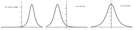
Figure 1.
Possible pdf shapes of the HSS model.
The quantile function for the HSS model is defined as
4. Estimation Methods
In this part, we will use several estimate methods to find the parameter estimators for our suggested models and . Estimation techniques are general processes that may be used to produce estimators in a parametric estimation issue. In general, these strategies determine the distribution or model parameters by maximizing or minimizing an objective function. In this paper, we will look at eight alternative estimating approaches to estimate the parameters of our model, as are shown below.
The maximum likelihood estimate approach is the first method (EM1). Our suggested model estimators and are produced using this strategy by maximizing the following equation:
Our suggested model estimators and are obtained using the Anderson–Darling estimation method (EM2) by minimizing the following equation:
The Cram’er-von Mises estimate is the third estimation method (EM3). In this strategy, we obtain our suggested model estimators and by minimizing the following equation:
The maximum product of the spacings estimation technique (EM4) is used to estimate and in the fourth approach. It is calculated by solving the following equation and maximizing it:
where
The least-squares estimating approach is the fifth method (EM5). Using this technique, the estimators of and are calculated by minimizing the following equation:
The percentile estimation technique (EM6) is used in the sixth approach to determine and by minimizing the following equation:
The right-tail Anderson–Darling estimating approach (EM7) is used to obtain our suggested model estimators and in the seventh approach. It is calculated by solving the following equation:
The weighted least-squares estimation technique (EM8) is used in the final procedure to construct the estimators of and by minimizing the following equation:
The performance of the various estimating approaches will be explored using numerical examples in the next section. The performance outcomes of the estimating methods might differ from one model to the next. In other words, the performance of an estimating approach may be the best in one situation for determining model parameters but not in another.
5. Numerical Simulation
This section investigates the performance of all of the estimating techniques mentioned in Section 4. We created random data sets using our proposed model, and we then used these estimation methods to discover the suggested model estimators. In this analysis, we utilize the three measures listed below to evaluate the performance of the estimation methods:
- The average of the absolute bias (BIAS), which is computed by .
- The mean squared errors (MSE), which is found using .
- The mean absolute relative errors (MRE), which is calculated using , .
Another goal of this simulation research is to determine the optimal estimate strategy for computing our suggested model estimators. We ran this simulation by producing random samples from our model of varying sizes and determining the measurements we employed; we then repeated that process thousands of times.
Table A1, Table A2, Table A3, Table A4 and Table A5 in Appendix A show the results of our simulation. We also display the values from these tables in Figure 2, Figure 3, Figure 4, Figure 5 and Figure 6. Figure 2, Figure 3, Figure 4, Figure 5 and Figure 6 show the performance outcomes for the eight different estimation methods; from these figures, we can generally see that, as the sample size increased, the measure decreased. The power of any value has been shown to be proportional to its position with respect to all of the estimating approaches. Table A6 shows our estimators’ partial and total ranks.
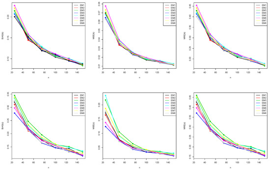
Figure 2.
Graphical representation of BIAS, MSE, and MRE values in Table A1.
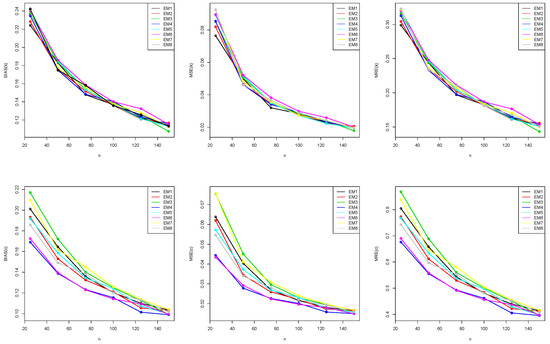
Figure 3.
Graphical representation of BIAS, MSE, and MRE values in Table A2.
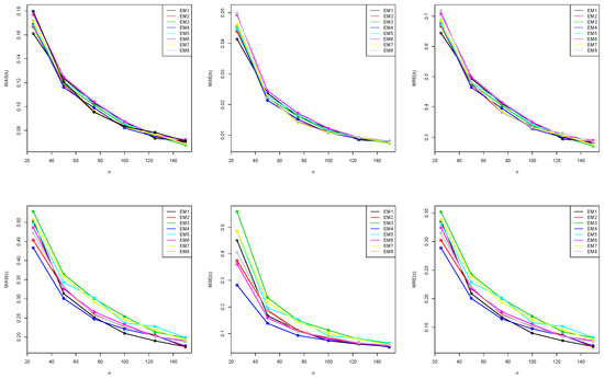
Figure 4.
Graphical representation of BIAS, MSE, and MRE values in Table A3.
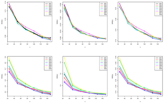
Figure 5.
Graphical representation of BIAS, MSE, and MRE values in Table A4.
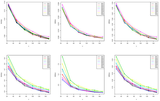
Figure 6.
Graphical representation of BIAS, MSE, and MRE values in Table A5.
In light of the outcomes obtained through simulation analysis and subsequent ranking assessments, several critical findings emerge:
- Consistency property of estimators: It was observed that all of the estimators under investigation demonstrated the property of consistency. This indicates that, as the sample size, denoted as ‘n’, increases, the estimators converge in probability to the true population parameter values. Such convergence lends robustness to these estimators, thus affirming their suitability for statistical inference tasks.
- Bias reduction with increasing sample size: For all of the considered estimating techniques, a discernible reduction in bias was discerned as the sample size ‘n’ increased. This finding underscores the beneficial impact of larger sample sizes on the accuracy and the unbiasedness of parameter estimation. This phenomenon can be attributed to the diminishing influence of random fluctuations in larger datasets.
- MSE minimization with growing sample size: An additional noteworthy observation was the diminishing trend in the MSE across all of the estimators as the sample size ‘n’ expanded. The MSE represents a comprehensive measure of the estimation performance, thereby incorporating both bias and variance components. The observed decline in the MSE underscores the improvement in the overall estimation precision with augmented sample sizes.
- Decreasing MRE with increasing sample size: Moreover, it became evident that the MRE decreased consistently across all of the estimating techniques as ‘n’ increased. The MRE provides insights into the relative accuracy of the estimators with respect to the true parameter values. A decline in the MRE indicates enhanced accuracy as larger data sets are utilized in the estimation process.
- Optimal estimation technique: Notably, the analysis revealed that the MPS estimation technique consistently outperformed other methods in terms of accuracy when estimating the parameters of interest. As a consequence, our empirical evidence strongly supports the adoption of the MPS approach by researchers dealing with data sets generated from the model proposed in this study. The MPS technique exhibited superior accuracy and reliability in parameter estimation, thereby constituting a highly recommended strategy for practitioners seeking precise parameter estimates.
- Finally, the findings derived from the simulation-based analysis presented in this study underscore the importance of the sample size in the context of parameter estimation. Furthermore, they provide empirical support for the preference of the MPS estimation technique over alternative methods, thus offering valuable guidance to researchers engaged in statistical modeling with data sets conforming to the model proposed herein.
6. Real Data Analysis
In this section, we consider the log returns of the Ethereum ERs real data set to illustrate the flexibility of the proposed distribution. It represents the daily Ethereum ERs based on USA dollars from 30 June 2017 to 30 June 2022. It is available on (https://www.google.com/finance/quote/ETH-USD).
To demonstrate how flexible the investigated models are, we will compare the proposed model to a number of well-known models, including the following: the type IV generalized logistic (IVGL) [23], Gumbel (Gu), Arctan Gumbel (AGu) [24], normal (Nr), Arctan normal (ANr) [24], beta-generalized logistic type IV (BGLIV) [25], and type II beta-generalized logistic (TIIBGL) [26] distributions.
The computed models were compared using some analytical measures, including information criteria (IC) such as the Akaike IC (AIC), corrected AIC (CAIC), and Hannan—Quinn IC (HQIC), as well as goodness-of-fit measures such as the Anderson—Darling (AD), Cramer—von Mises (CM), and Kolmogorov—Smirnov (KS) with its emphp value (KS emphp-value). In Table 1, the analytical measures, as well as the MLE and related standard errors (SEs), are presented in parenthesis for the analyzed real data set. We may deduce from this table that the proposed model fit better than the other models.

Table 1.
Numerical information criteria values with the goodness-of-fit measures for the Ethereum real data set.
The estimated PDF, CDF, SF, and P-P plots of the HS distribution for the real data set are shown in Figure 7. These results demonstrate that the proposed distribution is preferable for fitting the real data set. Figure 8 depicts the behavior of a log-likelihood function with the estimated parameters, which is a unimodal function with estimated parameters that are global maximum points. This means that they optimize the log-likelihood function and provide the best parameter estimates.
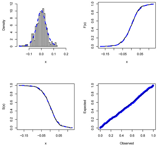
Figure 7.
Histogram of the Ethereum real data set with the fitted PDF, CDF, SF, and P-P plots.
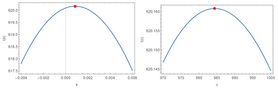
Figure 8.
The profile of the log-likelihood functions for k and c of the Ethereum real data set.
7. Conclusions
We have utilized the nonlinear evolution equation to construct a new probability density function of the hyperbolic secant (HS) distribution. This probability density function has been generated for the second family of solutions. We will consider the other two families in future work. Actually, this density function can be left-skewed, symmetric, or right-skewed. The behavior of the HS model parameters was investigated using these estimating techniques on randomly generated data sets using eight different frequent estimators for the parameters of our model. We extended our results to real-world data to demonstrate the HS distribution’s utility in simulating real data. To our knowledge, no other scientific work has ever presented the method that is being offered in this paper. Finally, a variety of other complex physical models can use the proposed motivation.
Author Contributions
A.F.D.: Conceptualization, Data curation, Formal analysis, Writing—original draft. A.M.T.A.E.-B.: Conceptualization, Data curation, Writing—review editing. A.M.G.: Conceptualization, Software, Formal analysis, Writing—original draft. M.A.E.A.: Conceptualization, Software, Formal analysis, Writing—review editing. S.Z.H.: Conceptualization, Data curation, Formal analysis, Writing—original draft. All authors have read and agreed to the published version of the manuscript.
Funding
The Deputyship for Research and Innovation via the Ministry of Education in Saudi Arabia provided funding this research work through the project number 445-9-339.
Data Availability Statement
The data used to support the findings of this study are included within the article.
Acknowledgments
The authors extend their appreciation to the Deputyship for Research and Innovation via the Ministry of Education in Saudi Arabia for funding this research work through the project number 445-9-339.
Conflicts of Interest
The authors declare that they have no competing interest.
Appendix A
Table A1.
Simulation values of BIAS, MSE, and MRE for .
Table A1.
Simulation values of BIAS, MSE, and MRE for .
| n | Est. | Est. Par. | ||||||||
|---|---|---|---|---|---|---|---|---|---|---|
| 25 | BIAS | |||||||||
| MSE | ||||||||||
| MRE | ||||||||||
| 50 | BIAS | |||||||||
| MSE | ||||||||||
| MRE | ||||||||||
| 75 | BIAS | |||||||||
| MSE | ||||||||||
| MRE | ||||||||||
| 100 | BIAS | |||||||||
| MSE | ||||||||||
| MRE | ||||||||||
| 125 | BIAS | |||||||||
| MSE | ||||||||||
| MRE | ||||||||||
| 150 | BIAS | |||||||||
| MSE | ||||||||||
| MRE | ||||||||||
Table A2.
Simulation values of BIAS, MSE, and MRE for .
Table A2.
Simulation values of BIAS, MSE, and MRE for .
| n | Est. | Est. Par. | ||||||||
|---|---|---|---|---|---|---|---|---|---|---|
| 25 | BIAS | |||||||||
| MSE | ||||||||||
| MRE | ||||||||||
| 50 | BIAS | |||||||||
| MSE | ||||||||||
| MRE | ||||||||||
| 75 | BIAS | |||||||||
| MSE | ||||||||||
| MRE | ||||||||||
| 100 | BIAS | |||||||||
| MSE | ||||||||||
| MRE | ||||||||||
| 125 | BIAS | |||||||||
| MSE | ||||||||||
| MRE | ||||||||||
| 150 | BIAS | |||||||||
| MSE | ||||||||||
| MRE | ||||||||||
Table A3.
Simulation values of BIAS, MSE, and MRE for .
Table A3.
Simulation values of BIAS, MSE, and MRE for .
| n | Est. | Est. Par. | ||||||||
|---|---|---|---|---|---|---|---|---|---|---|
| 25 | BIAS | |||||||||
| MSE | ||||||||||
| MRE | ||||||||||
| 50 | BIAS | |||||||||
| MSE | ||||||||||
| MRE | ||||||||||
| 75 | BIAS | |||||||||
| MSE | ||||||||||
| MRE | ||||||||||
| 100 | BIAS | |||||||||
| MSE | ||||||||||
| MRE | ||||||||||
| 125 | BIAS | |||||||||
| MSE | ||||||||||
| MRE | ||||||||||
| 150 | BIAS | |||||||||
| MSE | ||||||||||
| MRE | ||||||||||
Table A4.
Simulation values of BIAS, MSE, and MRE for .
Table A4.
Simulation values of BIAS, MSE, and MRE for .
| n | Est. | Est. Par. | ||||||||
|---|---|---|---|---|---|---|---|---|---|---|
| 25 | BIAS | |||||||||
| MSE | ||||||||||
| MRE | ||||||||||
| 50 | BIAS | |||||||||
| MSE | ||||||||||
| MRE | ||||||||||
| 75 | BIAS | |||||||||
| MSE | ||||||||||
| MRE | ||||||||||
| 100 | BIAS | |||||||||
| MSE | ||||||||||
| MRE | ||||||||||
| 125 | BIAS | |||||||||
| MSE | ||||||||||
| MRE | ||||||||||
| 150 | BIAS | |||||||||
| MSE | ||||||||||
| MRE | ||||||||||
Table A5.
Simulation values of BIAS, MSE, and MRE for .
Table A5.
Simulation values of BIAS, MSE, and MRE for .
| n | Est. | Est. Par. | ||||||||
|---|---|---|---|---|---|---|---|---|---|---|
| 25 | BIAS | |||||||||
| MSE | ||||||||||
| MRE | ||||||||||
| 50 | BIAS | |||||||||
| MSE | ||||||||||
| MRE | ||||||||||
| 75 | BIAS | |||||||||
| MSE | ||||||||||
| MRE | ||||||||||
| 100 | BIAS | |||||||||
| MSE | ||||||||||
| MRE | ||||||||||
| 125 | BIAS | |||||||||
| MSE | ||||||||||
| MRE | ||||||||||
| 150 | BIAS | |||||||||
| MSE | ||||||||||
| MRE | ||||||||||
Table A6.
Partial and overall ranks of all the methods of estimation of proposed distribution using various values of model parameters.
Table A6.
Partial and overall ranks of all the methods of estimation of proposed distribution using various values of model parameters.
| Parameter | n | ||||||||
|---|---|---|---|---|---|---|---|---|---|
| 25 | 4.0 | 3.0 | 7.5 | 1.0 | 5.0 | 6.0 | 7.5 | 2.0 | |
| 50 | 4.0 | 1.0 | 6.0 | 2.0 | 7.5 | 5.0 | 7.5 | 3.0 | |
| 75 | 3.0 | 6.0 | 8.0 | 1.5 | 7.0 | 4.0 | 5.0 | 1.5 | |
| 100 | 1.0 | 4.0 | 2.5 | 2.5 | 6.0 | 7.0 | 8.0 | 5.0 | |
| 125 | 5.0 | 4.0 | 8.0 | 1.0 | 7.0 | 6.0 | 3.0 | 2.0 | |
| 150 | 2.0 | 3.0 | 4.0 | 1.0 | 8.0 | 5.0 | 6.0 | 7.0 | |
| 25 | 3.0 | 3.0 | 7.0 | 1.0 | 5.0 | 3.0 | 8.0 | 6.0 | |
| 50 | 6.0 | 3.0 | 8.0 | 1.0 | 7.0 | 4.0 | 5.0 | 2.0 | |
| 75 | 2.5 | 2.5 | 6.0 | 1.0 | 4.0 | 5.0 | 8.0 | 7.0 | |
| 100 | 3.0 | 2.0 | 7.5 | 6.0 | 5.0 | 4.0 | 7.5 | 1.0 | |
| 125 | 4.0 | 1.0 | 5.0 | 3.0 | 2.0 | 6.0 | 8.0 | 7.0 | |
| 150 | 7.0 | 8.0 | 1.0 | 4.0 | 2.0 | 4.0 | 6.0 | 4.0 | |
| 25 | 3.0 | 1.0 | 8.0 | 2.0 | 4.0 | 5.0 | 7.0 | 6.0 | |
| 50 | 3.0 | 2.0 | 6.0 | 1.0 | 6.0 | 6.0 | 8.0 | 4.0 | |
| 75 | 4.5 | 3.0 | 6.5 | 2.0 | 8.0 | 6.5 | 4.5 | 1.0 | |
| 100 | 4.0 | 3.0 | 8.0 | 1.0 | 7.0 | 6.0 | 5.0 | 2.0 | |
| 125 | 1.0 | 4.0 | 5.0 | 2.0 | 8.0 | 3.0 | 7.0 | 6.0 | |
| 150 | 5.0 | 1.0 | 3.0 | 2.0 | 6.0 | 8.0 | 4.0 | 7.0 | |
| 25 | 6.0 | 3.0 | 8.0 | 1.0 | 4.0 | 5.0 | 7.0 | 2.0 | |
| 50 | 4.5 | 1.0 | 7.0 | 2.0 | 3.0 | 6.0 | 8.0 | 4.5 | |
| 75 | 4.5 | 1.0 | 8.0 | 2.0 | 3.0 | 6.0 | 7.0 | 4.5 | |
| 100 | 5.0 | 2.0 | 6.0 | 1.0 | 8.0 | 7.0 | 3.0 | 4.0 | |
| 125 | 2.0 | 4.0 | 7.0 | 1.0 | 5.0 | 6.0 | 8.0 | 3.0 | |
| 150 | 3.0 | 2.0 | 4.0 | 1.0 | 8.0 | 5.0 | 6.0 | 7.0 | |
| 25 | 4.0 | 1.0 | 8.0 | 2.0 | 3.0 | 6.0 | 5.0 | 7.0 | |
| 50 | 2.0 | 5.0 | 6.5 | 3.0 | 4.0 | 6.5 | 8.0 | 1.0 | |
| 75 | 4.0 | 2.5 | 5.0 | 1.0 | 6.0 | 7.0 | 8.0 | 2.5 | |
| 100 | 3.0 | 1.5 | 4.0 | 1.5 | 5.0 | 6.0 | 8.0 | 7.0 | |
| 125 | 1.0 | 2.0 | 8.0 | 3.0 | 5.0 | 6.0 | 7.0 | 4.0 | |
| 150 | 1.0 | 2.0 | 5.0 | 3.0 | 6.5 | 6.5 | 8.0 | 4.0 | |
| ∑ Rank | 105.0 | 81.5 | 183.5 | 56.5 | 165.0 | 166.5 | 198.0 | 124.0 | |
| Overall Rank | 3 | 2 | 7 | 1 | 5 | 6 | 8 | 4 |
References
- Mirzaee, F.; Rezaei, S.; Samadyar, N. Numerical solution of two-dimensional stochastic time-fractional sine-Gordon equation on non-rectangular domains using finite difference and meshfree methods. Eng. Anal. Bound. Elem. 2021, 127, 53–63. [Google Scholar] [CrossRef]
- Yamaguchi, R. Analysis of electro-optical behavior in liquid crystal cells with asymmetric anchoring strength. Symmetry 2022, 14, 85. [Google Scholar] [CrossRef]
- Alharbi, Y.F.; El-Shewy, E.K.; Abdelrahman, M.A.E. New and effective solitary applications in Schrödinger equation via Brownian motion process with physical coefficients of fiber optics. AIMS Math. 2023, 8, 4126–4140. [Google Scholar] [CrossRef]
- Yiasir Arafat, S.M.; Khan, K.; Rayhanul Islam, S.M.; Rahman, M.M. Parametric effects on paraxial nonlinear Schrödinger equation in Kerr media. Chin. J. Phys. 2023, 83, 361–378. [Google Scholar] [CrossRef]
- Ma, Y.L.; Li, B.Q. Kraenkel-Manna-Merle saturated ferromagnetic system: Darboux transformation and loop-like soliton excitations. Chaos Solitons Fractals 2022, 159, 112179. [Google Scholar] [CrossRef]
- Shakeel, M.; Iqbal, M.A.; Din, Q.; Hassan, Q.M.; Ayub, K. New exact solutions for coupled nonlinear system of ion sound and Langmuir waves. Indian J. Phys. 2020, 94, 885–894. [Google Scholar] [CrossRef]
- Matsushima, J.; Ali, M.Y.; Bouchaala, F. Propagation of waves with a wide range of frequencies in digital core samples and dynamic strain anomaly detection: Carbonate rock as a case study. Geophys. J. Int. 2021, 224, 340–354. [Google Scholar] [CrossRef]
- Younas, U.; Rezazadeh, H.; Ren, J.; Bilal, M. Propagation of diverse exact solitary wave solutions in separation phase of iron (Fe-Cr-X(X = Mo, Cu)) for the ternary alloys. Int. J. Mod. Phys. B 2022, 36, 2250039. [Google Scholar] [CrossRef]
- Tian, Q.; Yang, X.; Zhang, H.; Xu, D. An implicit robust numerical scheme with graded meshes for the modified Burgers model with nonlocal dynamic properties. Comput. Appl. Math. 2023, 42, 246. [Google Scholar] [CrossRef]
- Yang, X.; Wu, L.; Zhang, H. A space-time spectral order sinc-collocation method for the fourth-order nonlocal heat model arising in viscoelasticity. Appl. Math. Comput. 2023, 457, 128192. [Google Scholar] [CrossRef]
- Stuart, A.M. Inverse problems: A Bayesian perspective. Acta Numer. 2010, 19, 451–559. [Google Scholar] [CrossRef]
- Mirzaee, F.; Rezaei, S.; Samadyar, N. Solving one-dimensional nonlinear stochastic sine-Gordon equation with a new meshfree technique. Int. J. Numer. Model. 2021, 34, e2856. [Google Scholar] [CrossRef]
- de Bouard, A.; Debussche, A. Soliton dynamics for the Korteweg-de Vries equation with multiplicative homogeneous noise. Electron. J. Probab. 2009, 14, 1727–1744. [Google Scholar] [CrossRef]
- El-Wakil, S.A.; Elgarayhi, A.; Elhanbaly, A. Exact periodic wave solutions for some nonlinear partial differential equations. Chaos Solitons Fractals 2006, 29, 1037–1044. [Google Scholar] [CrossRef]
- Ablowitz, M.J.; Clarkson, P.A. Solitons, Nonlinear Evolution Equations and Inverse Scattering; Cambridge University Press: Cambridge, UK, 1991. [Google Scholar]
- El-Wakil, S.A.; El-labany, S.K.; Zahran, M.A.; Sabry, R. Modified extended tanh-function method for solving nonlinear partial differential equations. Phys. Lett. A 2002, 299, 179–188. [Google Scholar] [CrossRef]
- Yang, L.; Wang, D.; An, F. Exact solutions for generalized Klein-Gordon equation. J. Inform. Math. Sci. 2012, 4, 351–358. [Google Scholar]
- Nadarajah, S.; Kotz, S. Beta trigonometric distributions. Port. Econ. J. 2006, 5, 207–224. [Google Scholar] [CrossRef]
- Abd El-Bar, A.M.T.; Bakouch, H.S.; Chowdhury, S. A new trigonometric distribution with bounded support and an application. Rev. UnióN Matemática Argent. 2021, 62, 459–473. [Google Scholar] [CrossRef]
- Abate, J.; Choudhury, G.L.; Lucantoni, D.N.; Whitt, W. Asymptotic analysis of tail probabilities based on the computation of moments. Ann. Appl. Probab. 1995, 5, 983–1007. [Google Scholar] [CrossRef]
- Thongchan, P.; Bodhisuwan, W. A modified hyperbolic secant distribution. Songklanakarin J. Sci. Technol. 2017, 39, 11–18. [Google Scholar]
- Alomair, R.A.; Hassan, S.Z.; Abdelrahman, M.A.E. A new structure of solutions to the coupled nonlinear Maccari’s systems in plasma physics. AIMS Math. 2022, 7, 8588–8606. [Google Scholar] [CrossRef]
- Prentice, R.L. A generalization of the probit and logit methods for dose response curves. Biometrics 1976, 32, 761–768. [Google Scholar] [CrossRef] [PubMed]
- Alkhairy, I.; Nagy, M.; Muse, A.H.; Hussam, E. The Arctan-X family of distributions: Properties, simulation, and applications to actuarial sciences. Complexity 2021, 2021, 4689010. [Google Scholar] [CrossRef]
- Nassar, M.M.; Elmasry, A. A study of generalized logistic distributions. J. Egypt. Math. Soc. 2012, 20, 126–133. [Google Scholar] [CrossRef]
- Morais, A.L.; Cordeiro, G.M.; Cysneiros, A.H. The beta generalized logistic distribution. Braz. J. Probab. Stat. 2013, 27, 185–200. [Google Scholar] [CrossRef]
Disclaimer/Publisher’s Note: The statements, opinions and data contained in all publications are solely those of the individual author(s) and contributor(s) and not of MDPI and/or the editor(s). MDPI and/or the editor(s) disclaim responsibility for any injury to people or property resulting from any ideas, methods, instructions or products referred to in the content. |
© 2023 by the authors. Licensee MDPI, Basel, Switzerland. This article is an open access article distributed under the terms and conditions of the Creative Commons Attribution (CC BY) license (https://creativecommons.org/licenses/by/4.0/).