Optimization of Task-Scheduling Strategy in Edge Kubernetes Clusters Based on Deep Reinforcement Learning

Abstract

Kubernetes, known for its versatility in infrastructure management, rapid scalability, and ease of deployment, makes it an excellent platform for edge computing. However, its native scheduling algorithm struggles with load balancing, especially during peak task deployment in edge environments characterized by resource limitations and low latency demands. To address this issue, a proximal policy optimization with the least response time (PPO-LRT) algorithm was proposed in this paper. This deep reinforcement learning approach learns the pod-scheduling process, which can adaptively schedule edge tasks to the most suitable worker nodes with the shortest response time according to the current cluster load and pod state. To evaluate the effectiveness of the proposed algorithm, multiple virtual machines were created, and we built a heterogeneous node cluster. Additionally, we deployed k3s, a Kubernetes distribution suited for edge environments, on the cluster. The load balancing, high load resilience, and average response time during peak task deployment were tested by initiating numerous tasks within a limited time frame. The results validate that the PPO-LRT-based scheduler shows superior performance in cluster load balancing compared to the Kube scheduler. After the deployment of 500 random tasks, several cluster nodes become overwhelmed by using the Kube scheduler, whereas the PPO-LRT-based scheduler evenly allocates the workload across the cluster, reducing the average response time by approximately 31%.

1. Introduction

Edge computing is a decentralized computing model that brings computation and data processing closer to data sources and end-user devices. Its mission is to mitigate the data-transmission latency, ease network bandwidth constraints, and enhance real-time responsiveness and reliability. Servers, gateway devices, and intelligent terminals at the network edge handle computational tasks, meeting the demands of voluminous data and real-time applications. Task allocation in edge computing aims to optimally allocate tasks across suitable edge nodes, enhancing system performance and resource utilization. Its general workflow encompasses edge-node selection, a task-requirements analysis, a node evaluation, and a task-scheduling strategy.

The advantages of Kubernetes over other general edge-computing architectures are that it offers autoscaling capabilities and dynamically modifies the number of edge nodes based on workload shifts, thereby guaranteeing optimal resource use and efficient task execution. Kubernetes supports a variety of deployment modes, including a hybrid deployment of edge nodes and cloud data centers. This deployment and management flexibility of containerized applications in edge environments allows for the selection of the appropriate deployment methods based on specific needs, and it can also help automate the deployment, scaling, maintenance, and monitoring resources and applications in the edge-computing environment. This helps to simplify management tasks and reduce operational costs but introduces some challenges in the edge-computing architecture.

The Kube scheduler is a crucial Kubernetes component, responsible for scheduling pods (container groups) to suitable nodes for execution. The optimization of pod-scheduling algorithms in Kubernetes holds significant importance in improving cluster performance, resource utilization, reliability, and efficiency. With more intelligent scheduling algorithms, it becomes possible to better utilize the resources within the cluster, ensuring the optimal resource allocation to pods on nodes. This, in turn, reduces resource waste and enhances the overall cluster efficiency. By sensibly allocating pods across various nodes within the cluster, the application availability can be enhanced. In the event of a node failure, pods can be rescheduled onto other healthy nodes, ensuring the continuous operation of applications. Optimized scheduling algorithms can also consider the performance characteristics of nodes, scheduling pods onto the most suitable nodes to improve the application performance. Furthermore, better support for automation and autoscaling can be achieved by refining scheduling algorithms, enabling the cluster to automatically adjust resource allocation based on load conditions.

The default scheduling algorithm it uses involves rule-based rules, primarily focusing on factors like node resource availability, affinity, and anti-affinity rules for pod scheduling. These rules and algorithms are predetermined and cannot dynamically adjust to real-time environments and workload conditions. Traditional scheduling algorithms in the context of edge-task scheduling present several challenges:

Static Rules: Traditional algorithms typically employ static rules for scheduling, which cannot adapt flexibly to the swiftly changing requirements in edge environments. Frequent changes in node resources and network conditions in the edge environment make it challenging for traditional algorithms to optimize scheduling decisions based on real-time conditions.

Communication Cost: In edge computing, edge nodes are often spread across regions with weaker network connectivity, leading to higher communication costs compared to centralized cloud data centers. Traditional algorithms tend to schedule tasks to the cloud data center, resulting in underutilized edge node computational resources and increased data-transmission latency and network load.

Node Resource Imbalance: Traditional algorithms tend to assign tasks to nodes with ample resources, while edge nodes typically have limited resources. This could result in overloading some edge nodes while leaving others idle, leading to resource utilization imbalances.

Lack of Intelligent Decision Making: Traditional algorithms lack intelligent decision-making capabilities, making them unable to cater to specific task characteristics and requirements. Edge tasks may have varying real-time requirements, security needs, and location constraints, which traditional algorithms cannot accommodate.

Kubernetes scheduling algorithms can be primarily categorized into three types: rule-based optimization algorithms, metaheuristic algorithms, and intelligent predictive-scheduling algorithms. The rule-based optimization algorithms rely on affinity and antiaffinity scheduling, where Kubernetes facilitate defining relationships between pods and nodes by using labels and affinity rules, striving for refined resource allocation and node selection. Wöbker et al. [1] proposed a custom label system which was used by the schedulers for pod-to-node allocation. Medel et al. [2] used four labels for applications: high CPU utilization, low CPU utilization, high disk utilization, and low disk utilization. To prevent resource contention, containers with applications labeled as high utilization are not allocated to the same node. Lai et al. [3] concentrated on heuristic rule-based pod scheduling to optimize network latency in edge Kubernetes clusters, considering heterogeneous environments’ performance. However, these algorithms have a relatively singular optimization objective with limited adaptability, indicating potential for improvement in load balancing and capacity handling.

Metaheuristic algorithms are essential optimization algorithms for scientific workflow-scheduling problems, hybrid job-shop-scheduling problems, multiobjective decision-making problems, and so on. Tirkolaee et al. [4] designed a parallel heuristic algorithm that utilizes three prominent metaheuristic algorithms: a genetic algorithm (GA), particle swarm optimization (PSO), and ant colony optimization (ACO) to optimize the parallel job-scheduling problems, automated guided vehicles (AGVs), and transporters in a hybrid job-shop system. They found that parallel computing can enable heuristic algorithms to achieve better objective values. Goli et al. [5] discussed non permutation flow-shop-scheduling problems and proposed a novel multiobjective metaheuristic algorithm, providing pareto-optimal solutions in a shorter time. Kchaou [6] used interval type-2 fuzzy c-means (IT2FCM), a fuzzy clustering method, and PSO to optimize task scheduling while considering data placement. The concepts of multiobjective optimization and parallel computing in these algorithms can provide valuable insights for research on task-scheduling optimization in Kubernetes and edge computing.

The intelligent predictive-scheduling algorithms employ machine learning, reinforcement learning, and similar methods to anticipate node resource utilization based on historical data and trends. The goal is to enhance resource utilization and system performance. Park et al. [7] utilized a deep linear model (DLinear) to predict future resource usage based on collected resource utilization data and applied scoring to an efficient resource utilization (SERU) algorithm to allow it to select the best node. Ishak et al. [8] developed a scheduler for Kubernetes environments that uses machine learning methods based on a runtime prediction of applications, efficiently selecting the suitable device (CPU or GPU) for various tasks in heterogeneous systems. Kubernetes’ container-scheduling strategy (KCSS) [9] is a multicriteria decision-analysis algorithm that aggregates all the criteria into a single ranking and then chooses the node with the top rank to execute newly submitted containers. Deep reinforcement learning is a hot topic in edge architecture. Shi et al. [10] designed a task-offloading strategy based on a deep reinforcement learning algorithm. This strategy effectively enhances the long-term revenue for users when edge servers dynamically change service prices as users move. Yamansavascilar et al. [11] developed a task coordinator called DeepEdge based on deep reinforcement learning. It can learn offloading strategies to meet different task requirements under highly stochastic network conditions involving mobile users and applications without human intervention. Xiao et al. [12] proposed a reinforcement-learning-based mobile task-loading scheme for edge computing to counter interference attacks. This scheme employs secure reinforcement learning to avoid risky offloading strategies that cannot meet task computation latency requirements. Lim et al. [13] introduced a soft actor–critic (SAC) approach based on deep reinforcement learning to compute offloading decisions and facilitate multiaccess edge-computing (MEC) server decisions in a multiuser, multi-MEC server environment. Xu et al. [14] modeled the task offloading subproblem as an exact potential game (EPG) and proposed a multiagent distributed deep deterministic policy gradient (MAD4PG) algorithm to achieve Nash equilibrium.

Inspired by various deep reinforcement learning (DRL)-based edge-computing task-offloading and resource-allocation strategies, some research focuses on Kubernetes container-scheduling optimization in cloud environments by using reinforcement learning intelligent algorithms [15,16]. Jiaming [17] developed an RLSK job scheduler by using the deep Q learning network (DQN) algorithm, which adaptively schedules independent batch jobs across multiple federated cloud computing clusters. Peng [18] proposed the DL2 algorithm, a deep-learning-based scheduler for deep learning clusters, enhancing global training job scheduling by dynamically adjusting resource allocation for jobs. It outperforms other schedulers in terms of the average job-completion time.

After analyzing the current research on Kubernetes schedulers, we find that traditional scheduling strategies have difficulty adapting to the real-time and complex edge tasks. One key requirement in edge computing is the ability to make optimal decisions for future unknown tasks within an extremely short time frame. Conversely, existing predictive-scheduling strategies based on intelligent algorithms like machine learning and reinforcement learning effectively address adaptability and real-time issues. However, they have not been specifically designed and optimized for edge-device resource constraints, making them prone to device congestion during peak computing periods.

Deep reinforcement learning possesses features such as sample optimization, experience replay, function approximation, and model independence, making it highly suitable for dynamic environments like edge clusters and real-time task scheduling. Furthermore, the proximal policy optimization (PPO) algorithm, which uses a clipped function to restrict policy updates’ magnitude, speeds up the training’s convergence, reducing the training process’s load on edge clusters and enhancing the training efficiency. Therefore, a deep-reinforcement-learning-based proximal policy optimization with least response time (PPO-LRT) algorithm for enhancing pod scheduling in edge Kubernetes clusters was proposed in this paper. The PPO-LRT algorithm addresses cluster-load management in the context of heterogeneous edge environments, ensuring a more balanced cluster load during potential task peaks and reducing the maximum workload on worker nodes. To meet edge computing’s low-latency requirements, the LRT algorithm is integrated into the PPO’s reward function. This enables the model to make decisions with the shortest response time, decreasing the average response time of task-scheduling execution.

Our research contribution primarily revolves around modeling the Kubernetes pod-scheduling process as a Markov process, combining the PPO algorithm with the LRT algorithm to design Kubernetes pod-scheduling algorithms that are more suitable for edge environments. This achieves better load balancing and an increased load capacity. We also designed a reward function that facilitates a shorter scheduling time, leading to significant improvement in multiple objective optimizations. Furthermore, in terms of practical engineering, the custom scheduler we developed around the algorithm exhibits excellent maintainability and scalability.

The contributions are as follows:

• A Markov process for pod scheduling in edge heterogeneous environments using the k3s framework is modeled. A custom Kubernetes scheduler based on deep reinforcement learning is designed and implemented.
• The PPO-LRT algorithm is proposed by combining PPO with LRT. The reward function is designed to emphasize load balancing within the cluster and includes a mechanism to guard against excessively high workloads. Additionally, the algorithm incorporates a response time calculation, leading to more balanced loads on different nodes in the Kubernetes edge cluster and controlling resource utilization within a more reasonable range. This adaptive optimization addresses the resource constraints and low-latency requirements of the edge environment.
• The proposed PPO-LRT algorithm is implemented as a custom Kubernetes scheduler and interacts with the cluster. Different types and quantities of task sets are used to test the algorithm’s load-balancing adjustment capabilities and high-load bearing capacity in a heterogeneous and resource-limited cluster during task-scheduling peaks.

The remaining sections of this paper consist of the following: an overall architecture of the scheduling system based on deep reinforcement learning is described in Section 2. A Markov process modeling for Kubernetes task scheduling in edge environments is described and the PPO-LRT-scheduling algorithm is presented in Section 3. The evaluation experiments and analysis of the custom scheduler based on PPO-LRT are conducted in Section 4. Conclusions are drawn in Section 5.

2. Scheduling System Design

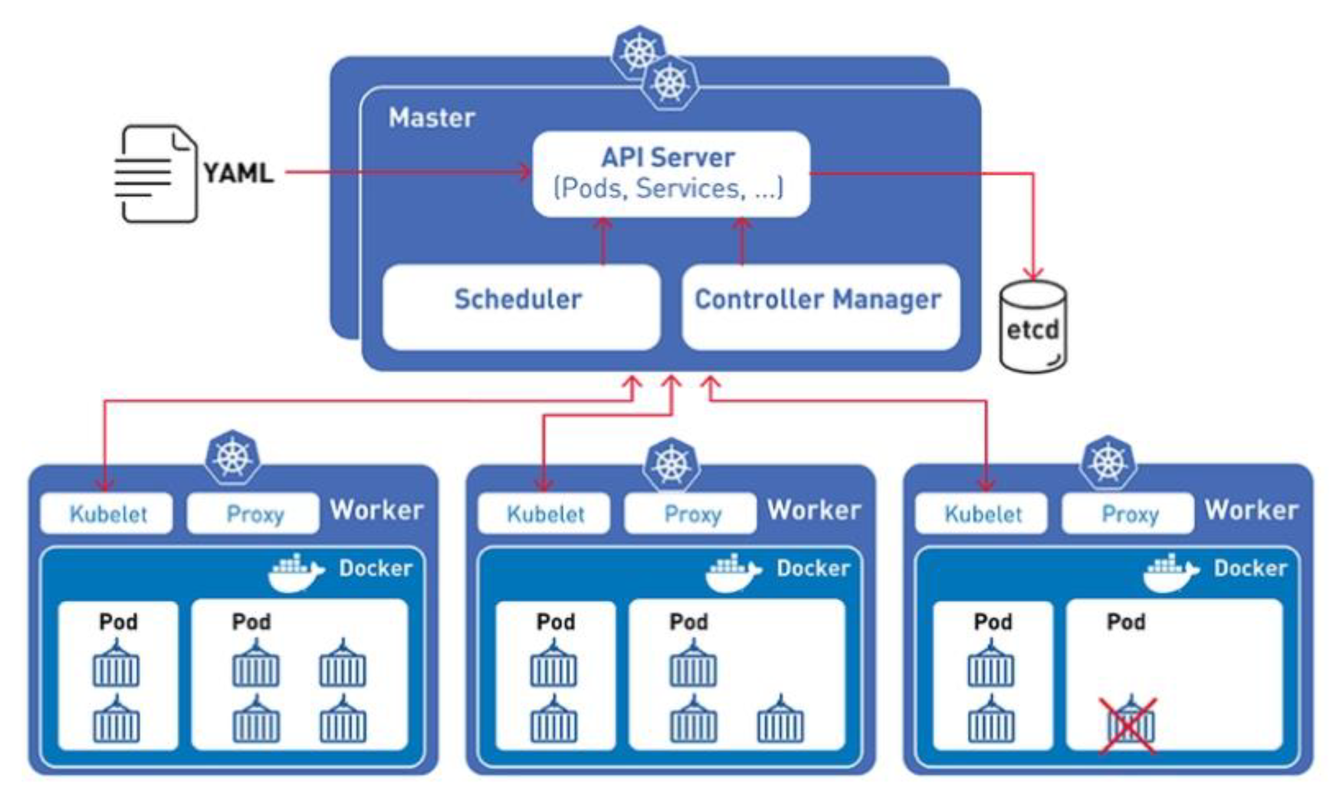
2.1. Kubernetes Cluster Architecture

The edge environment is a mesh of interconnected edge devices forming a multinode cluster environment. In such a setting, a distributed Kubernetes cluster architecture proves to be an excellent fit. Presently, Kubernetes boasts multiple distribution versions tailored for edge environments, such as k3s and KubeEdge. These distributions are Kubernetes architecture-based, supporting collaborative edge-computing nodes, task orchestration, and scheduling abilities on the edge-computing platform. Moreover, they are compatible with the requisite technical interfaces of the Kubernetes framework, which enables the use of identical interfaces for operations like gathering the node status or deploying pods.

As depicted in Figure 1, the node cluster within the Kubernetes framework includes both a master node and multiple worker nodes. The worker nodes operate as the working cells of the cluster where containers execute. The master node acts as the cluster control plane, handling the management and oversight of the overall cluster states and scheduling. Typically, it comprises several core components, including the API server, etcd, scheduler, and controller manager. Among these, the scheduler is the critical component responsible for task scheduling within the Kubernetes cluster. It allocates containerized applications (pods) to execute on nodes based on user-defined requirements and cluster-resource availability. The scheduler’s primary objectives are to maximize cluster resource utilization and ensure a high availability and application performance [19]. These are achieved by monitoring the cluster states, tracking resource usage, and making decisions per the defined scheduling policies. The scheduler is pluggable and can be customized or extended as per user requirements. Kubernetes provides various ways to implement custom schedulers such as modifying the Kube-scheduler source code, implementing extended schedulers, or creating custom score plugins in the scheduling framework [20,21].

Considering the interaction between the deep reinforcement learning program and the cluster, and with an eye on future algorithm optimization iterations and custom scheduler maintenance and updates, a custom scheduler using the extended scheduler approach is implemented, using HTTP/S calls to the Kubernetes API to enable an interaction between the scheduler and the cluster during the training and scheduling processes.

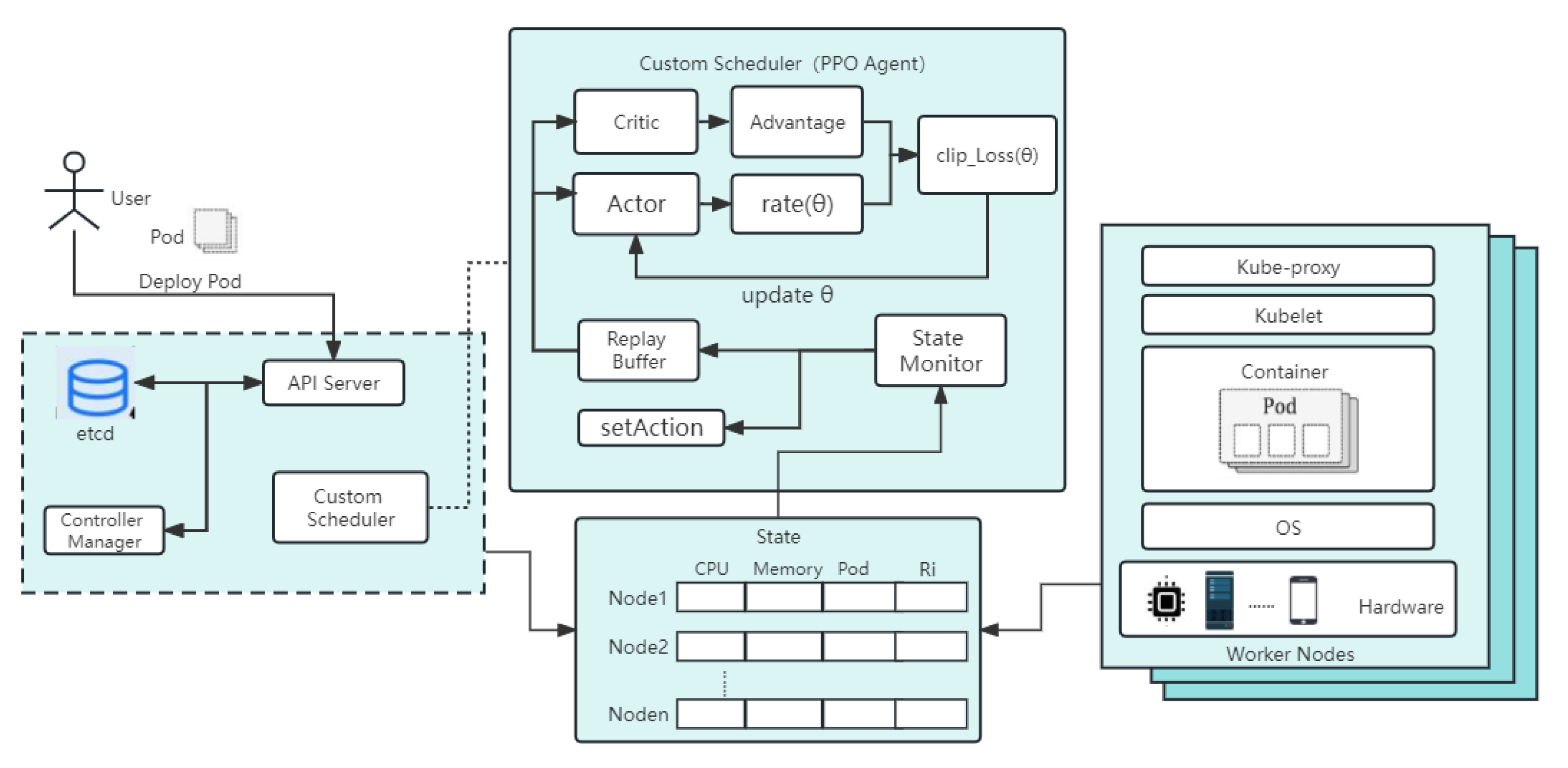
2.2. Custom Scheduler Design Based on DRL

A scheduling policy-optimization training program based on the PPO-LRT algorithm is set forth and a scheduler is developed subsequently in this study. The schematic of the Kubernetes scheduler based on the PPO-LRT algorithm is shown in Figure 2. When a user wishes to deploy a pod, a request with resource requirements for the CPU, memory, and other resources is forwarded to the API server component of the master. These data inform the initial node selection by the scheduler. The custom scheduler operates as an external scheduler, interacting with the master node via the HTTP protocol. This methodology offers more flexibility and maintainability compared to direct modifications of the default scheduler. It allows for cooperation with the default scheduler, or it can work independently as a custom scheduler. The PPO agent, responsible for policy optimization, employs the state monitor component to continuously track the cluster’s state and subsequently train the actor–critic network for improved policy decision making. To ensure stable and efficient policy updates within the PPO-LRT algorithm, the clip-loss function is employed to limit drastic changes in the policy. Finally, the trained optimal policy is incorporated into the custom scheduler, either as a replacement or supplement to the default Kubernetes scheduler. The ultimate objective is to achieve a balanced cluster load and optimized resource utilization.

In the scheduling architecture, the cluster consists of four nodes, including one master node and four worker nodes. The master node also acts as a worker node. Each node has different CPU and memory capacities to simulate a heterogeneous edge environment. During the task-scheduling phase, the default scheduler is bypassed and the custom scheduler is employed for scheduling. The custom scheduler uses the PPO deep reinforcement learning algorithm to train optimal scheduling policies to deploy pod applications based on user-defined resource requirements. Concurrently, it continually monitors the cluster’s states, making timely adjustments to overloaded nodes to ensure that the entire cluster and each node maintain reasonable resource utilization and load allocation.

The workload for testing comprises batch-created pods, and the pods’ configuration files define the required resource information, which is also part of the cluster’s state. To adapt to the deep reinforcement learning algorithm, the task-scheduling and workload-management problem in the Kubernetes cluster is characterized as a Markov decision process. Based on the PPO algorithm, the interaction and training process between the agent and the Kubernetes cluster are defined. This process is realized through the custom scheduler, integrating state monitoring, reinforcement learning training, and task deployment execution. The agent communicates with the cluster and performs pod control operations via the HTTP protocol and the Kubernetes API. The timing diagram illustrating the interaction between the custom scheduler based on PPO-LRT and other modules during the training process is shown in Figure 3.

3. PPO-LRT Algorithm

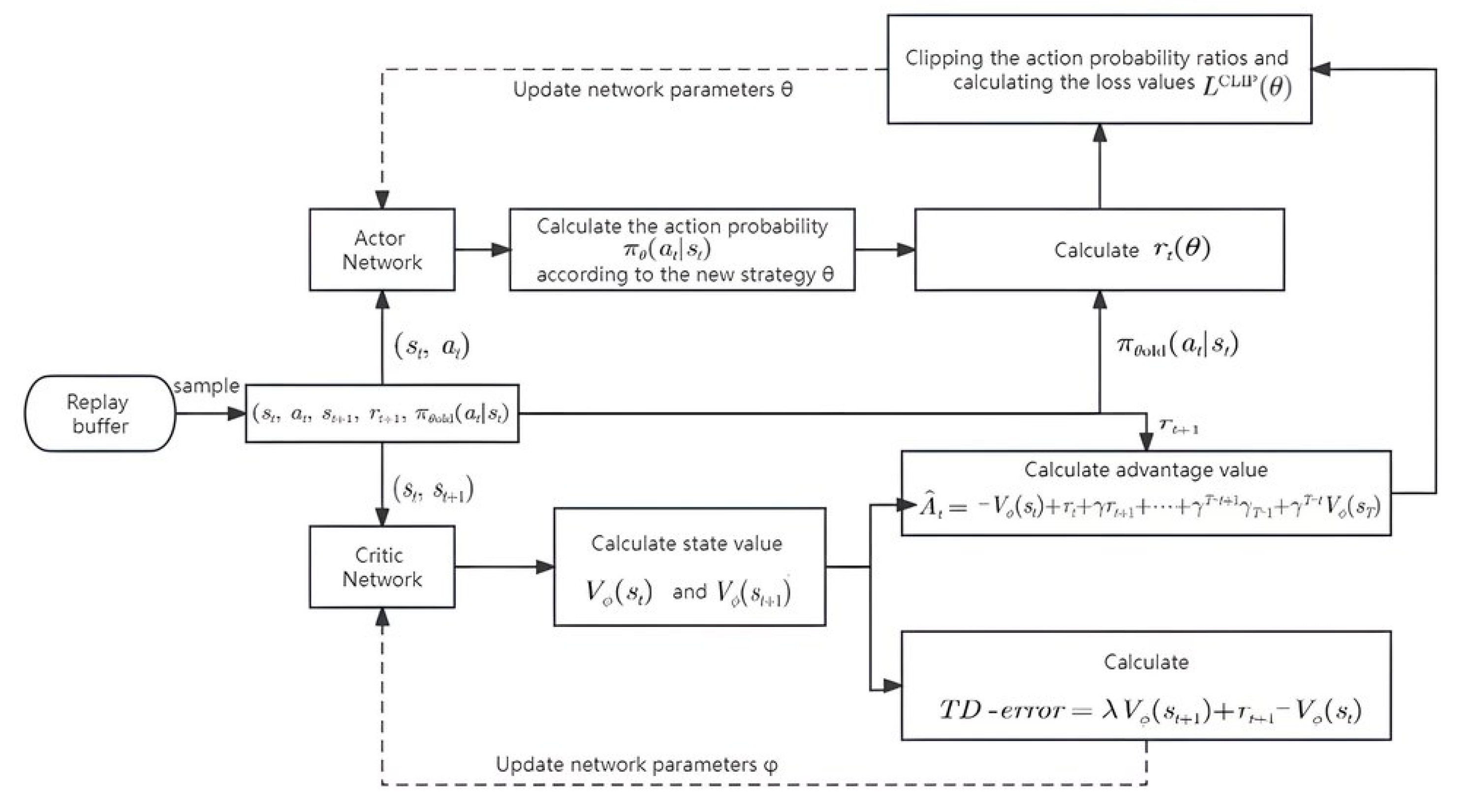
Whether in the traditional edge-computing architecture or edge-Kubernetes framework, task offloading and scheduling are dynamic and highly uncertain processes. Faced with the unstable dynamic cluster load states, PPO’s clipping algorithm can offer a relatively stable training process and faster convergence speed. Secondly, it demonstrates a higher training efficiency with fewer samples, which aligns well with resource-constrained edge environments. Additionally, in our scheduling problem, the action space is discrete, and when there are numerous nodes and extensive load parameters, the dimensionality of the collected state space also increases. For other algorithms suitable for discrete action spaces, the estimation of the value function typically becomes more complex. This might make it challenging to run the algorithm on edge devices since edge devices may not provide powerful computational capabilities. Therefore, as a policy gradient-based algorithm with clipping properties, PPO is better suited for dynamic edge environments.

3.1. PPO Algorithm

In the realm of deep reinforcement learning, an intelligent agent utilizes a deep neural network as its policy function to learn decision-making strategies. The agent examines the state and employs the neural network to estimate the value or probability distribution of each possible action. Following the estimated value or probability distribution, the agent opts for an action and interacts with its environment.

The deep neural network of the agent undergoes training and optimization by using the backpropagation algorithm. This process reduces the gap between the predicted value and actual reward (loss function), progressively refining the policy function. Consequently, the agent becomes more capable of garnering higher cumulative rewards within the environment [22].

The PPO algorithm used in this study is an algorithm dedicated to policy optimization for reinforcement learning. It aims to ensure stable policy improvement and maintain a high sample efficiency during the optimization process by restricting the magnitude of the policy updates and preventing drastic changes in the policy [23]. During the training process, the intelligent agent first interacts with the environment and collects a batch of trajectory data. It then uses the collected data to calculate the clipped surrogate objective and optimize the policy network and the value function network to improve the accuracy of the value function.

The optimization objective of PPO can be expressed as follows [23]:

$$J(\pi )={\mathbb{E}}_{s_0\sim {\rho }_0}\left[V_{\pi }\left(s_0\right)\right]$$

(1)

where $s_0$ represents the initial state, ${\rho }_0$ represents the initial state distribution, and $V_{\pi }\left(s_0\right)$ represents the state-value function under policy $\pi$. During the learning process, the relationship between the new policy ${\pi }_{\mathrm{n}\mathrm{e}\mathrm{w}}$ and the old policy ${\pi }_{\mathrm{o}\mathrm{l}\mathrm{d}}$ after each policy update can be represented as follows [24]:

$$J\left({\pi }_{\mathrm{new}}\right)=J\left({\pi }_{\mathrm{old}}\right)+{\mathbb{E}}_{s_0,a_0,s_1,a_1,\dots }\left[\sum _{t=0}^{\infty }{\gamma }^t{A}_{{\pi }_{\mathrm{old}}}\left(s_t,a_t\right)\right]$$

(2)

where $s_0\sim {\rho }_0,a_t\sim {\pi }_{\mathrm{new}}\left(\cdot |s_t\right),\hspace{1em}{s}_{t+1}\sim P\left(s_{t+1}|s_t,a_t\right),P\left(s_{t+1}|s_t,a_t\right)$ represents the environmental transition probability, γ is the discount factor, and $A_{\pi }\left(s_t,a_t\right)$ is the advantage function. As derived from Equation (2),

$$\begin{array}{c}J\left({\pi }_{\mathrm{new}}\right)-J\left({\pi }_{\mathrm{old}}\right)\ge \\ \frac{1}{1-\gamma }\underset{\begin{array}{c}s\sim D^{{\pi }_{\mathrm{old}}}\\ a\sim {\pi }_{\mathrm{old}}\end{array}}{\mathbb{E}}\left[\frac{{\pi }_{\mathrm{new}}(a|s)}{{\pi }_{\mathrm{old}}(a|s)}{A}^{{\pi }_{\mathrm{old}}}(s,a)\right]-\frac{\gamma ϵ}{{(1-\gamma )}^2}\underset{\begin{array}{c}s\sim D^{{\pi }_{\mathrm{old}}}\\ a\sim {\pi }_{\mathrm{old}}\end{array}}{\mathbb{E}}\left[\left|\frac{{\pi }_{\mathrm{new}}(a|s)}{{\pi }_{\mathrm{old}}(a|s)}-1\right|\right]\end{array}$$

(3)

In (3), the right-hand side of the inequality represents the lower bound of policy improvement, denoted as the policy improvement lower bound (PILB). The first term is the surrogate objective (SO), and the second term is the penalty term (PT). A policy improvement is made at each time as long as the lower bound of the policy improvement is positive, i.e., PILB = SO − PT ≥ 0, which ensures that the new policy is better than the old policy. To achieve this goal, it is necessary to enhance the SO while keeping the difference between the new and old policies relatively small, i.e.,

$$\begin{array}{c}\underset{{\pi }_{\mathrm{new}}}{maximize}\underset{\begin{array}{c}s\sim D^{{\pi }_{\mathrm{old}}}\\ a\sim {\pi }_{\mathrm{old}}\end{array}}{\mathbb{E}}\left[\frac{{\pi }_{\mathrm{new}}(a|s)}{{\pi }_{\mathrm{old}}(a|s)}{A}^{{\pi }_{\mathrm{old}}}(s,a)\right]\\ \mathrm{s}.\mathrm{t}.\underset{\begin{array}{c}s\sim D^{{\pi }_{\mathrm{old}}}\\ a\sim {\pi }_{\mathrm{old}}\end{array}}{\mathbb{E}}\left[\left|\frac{{\pi }_{\mathrm{new}}(a|s)}{{\pi }_{\mathrm{old}}(a|s)}-1\right|\right]\le \delta \end{array}$$

(4)

Because the distribution $D^{{\pi }_{\mathrm{old}}}$ in Equation (4) cannot be accurately computed, it is approximated by using the trajectory ${\pi }_{\mathrm{old}}$ generated by interacting with the environment. Additionally, if the policy is parameterized as ${\pi }_{\theta }$, the optimization problem in Equation (4) can be approximated by solving the optimization problem shown in Equation (5):

$$\begin{array}{c}\underset{\theta }{maximize}\underset{(s,a)\sim {\tau }_{\mathrm{old}}}{\mathbb{E}}\left[\frac{{\pi }_{\theta }(a|s)}{{\pi }_{{\theta }_{\mathrm{old}}}(a|s)}{A}^{{\pi }_{{\theta }_{\mathrm{old}}}}(s,a)\right]\\ \mathrm{s}.\mathrm{t}.\underset{(s,a)\sim {\tau }_{\mathrm{old}}}{\mathbb{E}}\left[\left|\frac{{\pi }_{\theta }(a|s)}{{\pi }_{{\theta }_{\mathrm{old}}}(a|s)}-1\right|\right]\le \delta \end{array}$$

(5)

The whole process is described in Figure 4. The algorithm quantifies the ratio of the new and old policies, denoted as $r_t\left(\theta \right)$, in the actor network and computes the advantage value ${\hat{A}}_t$ by utilizing the value function in the critic network. These values are then incorporated into the clipping function to evaluate the loss value $L^{\mathrm{C}\mathrm{L}\mathrm{I}\mathrm{P}}\left(\theta \right)$, as shown in Equations (6) and (7). It should be noted specifically that maximizing the objective function in Equation (7) can be considered as a further solution to the optimization problem in Equation (5), where ${\hat{A}}_t=A^{{\pi }_{{\theta }_{\mathrm{old}}}}(s,a)$. The other abbreviations in Figure 4 are defined in

Table 1. Parameter description.

Definition	Description
$r_t\left(\theta \right)$	Ratio of the new and old policies
$L^{\mathrm{C}\mathrm{L}\mathrm{I}\mathrm{P}}\left(\theta \right)$	Loss function based on clip function
$\theta$	Policy network parameter
$a_t$	The action at the moment t
$s_t$	The state at the moment t
$\epsilon$	Hyperparameter between 0 and 1
${{\displaystyle V}}_{\mathsf{\Phi }}(s)$	A value function in state $s_t$ that estimates the expected return of following a strategy in that state, where φ is a parameter of the value function, usually a neural network or other learning model
${\pi }_{\theta }\left(a_t\mid s_t\right)$	Probability of executing $a_t$ state $s_t$

. The PPO algorithm is a policy-optimization mechanism for reinforcement learning that curbs the degree of policy updates through approximate policy optimization and value-function optimization. This results in a steady, efficient policy improvement accompanied by a high sample efficiency and robust convergence performance:

$$r_t(\theta )=\frac{{\pi }_{\theta }\left(a_t\mid s_t\right)}{{\pi }_{\theta \mathrm{old} }\left(a_t\mid s_t\right)}$$

(6)

$$\begin{array}{c}{L}^{\mathrm{C}\mathrm{L}\mathrm{I}\mathrm{P}}(\theta )=\underset{(s,a)\sim {\tau }_{\mathrm{old}}}{\mathbb{E}}\left[min\left(r_t(\theta ){\hat{A}}_t,\mathrm{c}\mathrm{l}\mathrm{i}\mathrm{p}\left(r_t\left(\theta \right),1-\epsilon ,1+\epsilon \right){\hat{A}}_t\right)\right]\end{array}$$

(7)

3.2. Least Response Time (LRT)

The least response time (LRT) algorithm works by estimating each task’s response time based on its arrival and execution time. It then arranges the tasks by their response time [25]. The LRT algorithm follows these steps:

Task Arrival: the system records the arrival time of each task.

Compute Response Time: for each task, the response time is calculated as the sum of the task’s arrival time and its execution time.

Sort Tasks: the system sorts all tasks based on their response time, putting the task with the shortest response time first.

Execute Tasks: the tasks are executed according to the order set by the sorted response time.

The key to the LRT algorithm lies in its response time calculation $R_i=A_i+E_i$, where $A_i$ is the time from task i‘s creation to its scheduled state, i.e., the time from ‘container creating’ to the ‘pod scheduled’ state, and $E_i$ is the execution time of task i. The response time also reflects the cluster’s current load status, including network and disk loads.

LRT’s advantage is its ability to prioritize tasks with a shorter response time, thus diminishing the task waiting time. For this study, the LRT algorithm’s idea is incorporated into the reward function of PPO, creating the PPO-LRT algorithm. Although the LRT algorithm might not be ideal for real-time dynamic task scheduling, it can enhance load balancing and speed up the response time when combined with deep-reinforcement-learning-based real-time dynamic task-scheduling algorithms.

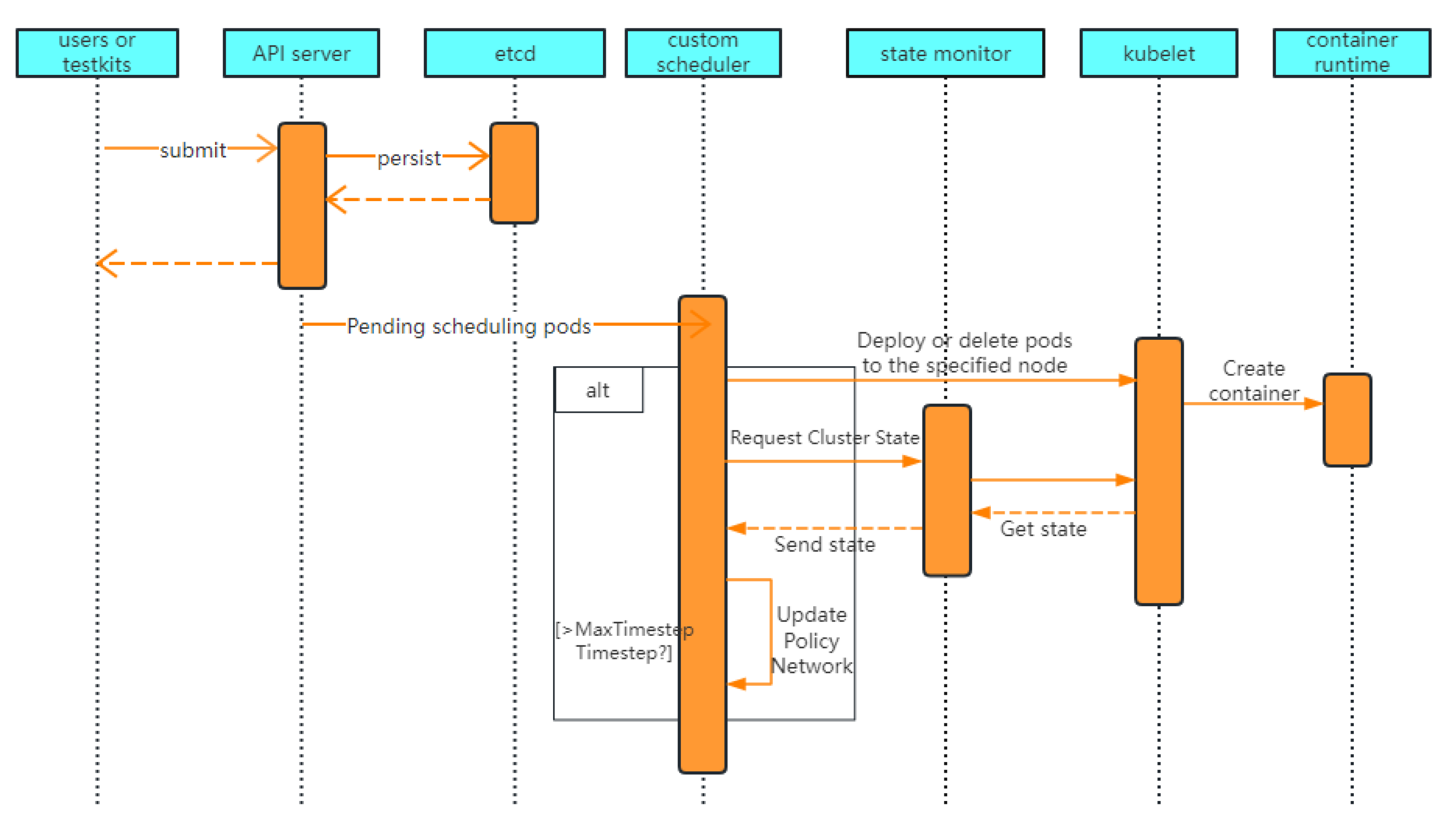
3.3. Scheduling Problem Modeling and PPO-LRT Algorithm Flow

The test workload generator is cyclically created, and the pods are deployed to the cluster based on the number of required training iterations and the effective operations. Following the deployment of the corresponding pod, the agent gathers the cluster state through a state-monitoring program, generating the state required for reinforcement learning training. The state considers factors such as the CPU load, memory utilization, and resource requirements (including CPU and memory demands) as specified in the pod configuration files. It also considers the response time of past pods. The state space is defined as follows:

$$state\left(t\right)=\left[{node}_1,{node}_2,\dots {node}_n,pod,r\right]$$

(8)

where ${node}_n$ is the state information of the n-th node in the cluster. Each ${node}_n$ state consists of four elements, where $c_n$ and $m_n$ represent the CPU load and memory utilization of the n-th node, respectively.${cp}_n$ and ${mp}_n$ represent the CPU and memory resource requirements for a pod running on n nodes, respectively. Their definitions are provided in Equation (9). The resource demands of pods are also a critical factor to be considered during scheduling, so in the state space, the pod is defined as the resource requirements of the currently deployed pod on the allocated node, which includes CPU and memory. Additionally, R represents the response time of the previous pod, defined in Equation (10):

$${node}_n=\left[c_n,m_n\right]$$

(9)

$$pod=[{cp}_n,{mp}_n]$$

(10)

Considering the optimization goals for pod-task scheduling and cluster-load balancing, the agent’s actions are designed into two categories: scheduling actions and load control actions. Scheduling actions entail selecting the node where a pod should be allocated. The output of the action decision is the node index (node). After acquiring the scheduling action, load control actions are ascertained based on the current load balance and resource utilization of each node. This involves deciding whether to deploy or remove some of the load. Within the cluster, the number of nodes is n, so the action space dimension is 2n, as shown in Equation (11):

$$action=\left[a_1,a_2\dots a_n\right]$$

$$a_n=[n,mod(n,2\left)\right]$$

(11)

where n denotes the node index. In the $a_n$ sequence, the first element indicates the node index where the agent’s load control action decision will be executed, symbolized as ${node}_n$. The second element is obtained by using the modulo function, where n is divided by two to yield a binary value representing the choice between scheduling and deploying pods or clearing some pods.

The reward function is designed based on the optimization goals. It incentivizes smaller load imbalances and shorter response time among clusters while ensuring that resource utilization stays within a reasonable range. The reward function also penalizes scenarios where resource utilization is excessively high. This is to achieve the objectives of load balancing control and optimizing resource utilization. The reward function is defined as follows:

$$reward=\alpha \times (\frac{1}{{\sigma }_c}+\frac{1}{{\sigma }_m})-\beta \times p-\gamma R_i$$

(12)

where α, β, and γ are the weights; p is the penalty value; $R_i$ denotes the task response time; and ${\sigma }_c$ is the dispersion of CPU loads across all nodes. The sequence [$c_1,c_2\dots c_n]$ represents the CPU load status values of n nodes, and ${\sigma }_c$ is the standard deviation of this sequence calculated according to Equation (13). The dispersion of the memory utilization sequence for all nodes ${\sigma }_m$ can be calculated similarly:

$${\sigma }_c=\sqrt{\frac{{\sum }_{i=1}^n{\left(c_i-\mathsf{\mu }\right)}^2}{n}}$$

(13)

Let $l_c$ $l_m$ represent the upper limit values of the reasonable range for CPU and memory, respectively. When the individual load status value surpasses the upper limit, the difference between the load status value and the upper limit is calculated as the penalty value. The penalty values for the CPU load $p_c$ are calculated according to Equation (14). The penalty values for the memory load $p_m$ can be calculated similarly:

$$p_c=\sum _{i=1}^n\left\{\left(c_i-l_c\right)|c_i>l_c\right\}$$

(14)

We set 300 episodes for training, and each episode contains 10 timesteps. Since a single pod has a limited impact on the cluster state, deploying only one pod in each training iteration may lead to small differences in the rewards between iterations, affecting the training speed and effectiveness. To mitigate this, we cyclically deploy 10 pods in each timestep, ensuring more substantial changes in the state with each deployment. The response time and resource demands of the tasks within the pods are randomized to simulate a more realistic and stochastic workload. The timespan of each iteration is determined by the completion time of all tasks, which also introduces randomness. After successfully scheduling all tasks to various nodes in the cluster, the agent interacts with the Kubelet through the Kube-Prometheus interface to obtain the cluster status data and gather response-time statistics. After a certain number of iterations, the training trajectory sequence $D_k$ is obtained, which includes the action (the scheduling result), the post scheduling cluster state, the instantaneous reward, and the response time for each iteration. The critic and actor networks are continuously updated by calculating the advantage function and maximizing the surrogate objective function with clipped values. At the end of each training iteration, the latest policy’s behavior decision is executed in the cluster through the “setAction” module within the agent, using the Kubernetes API to interact with the cluster. Algorithm 1 outlines the process of training the custom scheduler’s scheduling strategy by using the PPO-LRT algorithm with the batched deployment of tasks.

Algorithm 1 Pod Scheduling Algorithm Based on PPO-LRT

Initialize the policy parameters θ.

Initialize the value function network parameters ϕ.

for i in range(t):

Perform the scheduling of a certain number of pods based on the current policy ${\pi }_{\theta }$ and obtain trajectories $D_k=\left\{{\tau }_i\right\}$.

Calculate the rewards-to-go $\widehat{R_t}$ using Equation (5).

Obtain the current state data of all nodes in the cluster, including CPU, memory, resource requirements of the previous pod, and its response time. Then, use the current value function $V_{{\varnothing }_k}$ to estimate the advantage values $\widehat{A_t}$ of the trajectory data.

Updating the policy by maximizing the clipped surrogate objective function:

$L^{CLIP}\left(\theta \right)={\widehat{\mathbb{E}}}_t\left[min\left(r_t\left(\theta \right){\hat{A}}_t,\mathrm{clip}\left(r_t\left(\theta \right),1-ϵ,1+ϵ\right){\hat{A}}_t\right)\right]$

where $r_t\left(\theta \right)={\mathsf{\pi }}_{\theta }(\mathrm{a}|\mathrm{s})/{\mathsf{\pi }}_{\mathsf{\theta }\_\mathrm{old}}(\mathrm{a}|\mathrm{s})$, $\epsilon$ is a hyperparameter.

The value function is updated by minimizing the mean squared error between the predicted values and the observed returns:

${\varphi }_{k+1}=\arg \underset{\varphi }{min}\frac{1}{\left|{\mathcal{D}}_k\right|T}{\displaystyle \sum _{\tau \in {\mathcal{D}}_k}}{\displaystyle \sum _{t=0}^T}{\left(V_{\varphi }\left(s_t\right)-{\hat{R}}_t\right)}^2$.

Use the updated policy to repeat the process.

4. Evaluation

The effectiveness of the PPO-LRT algorithm in achieving load balancing and improving the overall task response time was evaluated. The experimental environment and test workloads were introduced at first. Since the default scheduler in the Kube scheduler has already considered priority-based preemption and load-based scoring algorithms, which are more comprehensive than traditional random and round-robin load-scheduling algorithms, the Kube scheduler was used as a comparative benchmark to evaluate the performance of the PPO-LRT algorithm in this paper.

4.1. Experimental Environment Setup

The experimental environment consists of four virtual machines, each simulating a node with differing CPU performances, memory sizes, and operating systems. Some nodes have constrained CPU and memory resources to mimic the conditions of heterogeneous and resource-restricted devices commonly found in edge environments. The virtual machines were interconnected, offering memory capacities between 3 GB and 8 GB. The master node, which acts as both the management and worker node, was allocated the maximum memory and CPU cores. Each of the other three worker nodes were assigned two CPU cores. Together, a four-node k3s edge device cluster running k3s version 1.22.6 was formed. The experimental environment is shown in

Table 2. Experimental environment.

Node	OS	CPU Cores	Memory
Master (Node1)	Centos7	8	8 GB
Node2	Centos7	2	3 GB
Node3	Ubuntu	2	4 GB
Node4	Redhat	2	4 GB

.

For the experiment, we employed two types of load-testing modes: balanced and random load testing. For the balanced load testing, we cyclically deployed Nginx as a single load during reinforcement learning training. For the random load testing, we used the PolybenchC benchmark suite to generate the random workload. PolybenchC, a comprehensive computer-system-performance evaluation suite, is typically used to gauge the effects of compiler optimization and parallel computing. It consists of a collection of C-language kernels representing common numerical computation algorithms, including matrix multiplication, matrix transpose, linear equation solving, and so on. We randomly selected 10 representative test programs from various types of computations in PolybenchC and packaged each program into a Docker image. These were then available to be pulled as test task sets when generating the pods. The benchmarks in PolybenchC vary greatly in resource requirements, such as CPU and memory, making it ideal for simulating the optimization effects of the PPO-LRT algorithm on Kubernetes cluster load under different task types. The specific test sets used, along with their computational types, are listed in

Table 3. Random load test programs (PolybenchC).

Name	Type	Description
Jacobi-2d	Linear Algebra	2D Jacobi stencil computation
3 mm	Linear Algebra	Three matrix multiplications
2 mm	Linear Algebra	Two matrix multiplications
Gemm	Linear algebra	Matrix multiplication
Atax	Linear Algebra	Matrix transpose and vector multiplication
Cholesky	Linear Algebra	Cholesky decomposition
heat-3d	Physics simulation	Heat equation over 3D data domain
Fdtd-2d	Physics simulation	2D finite-difference time-domain kernel
Covariance	Data mining	Covariance computation
Correlation	Data mining	Correlation computation

.

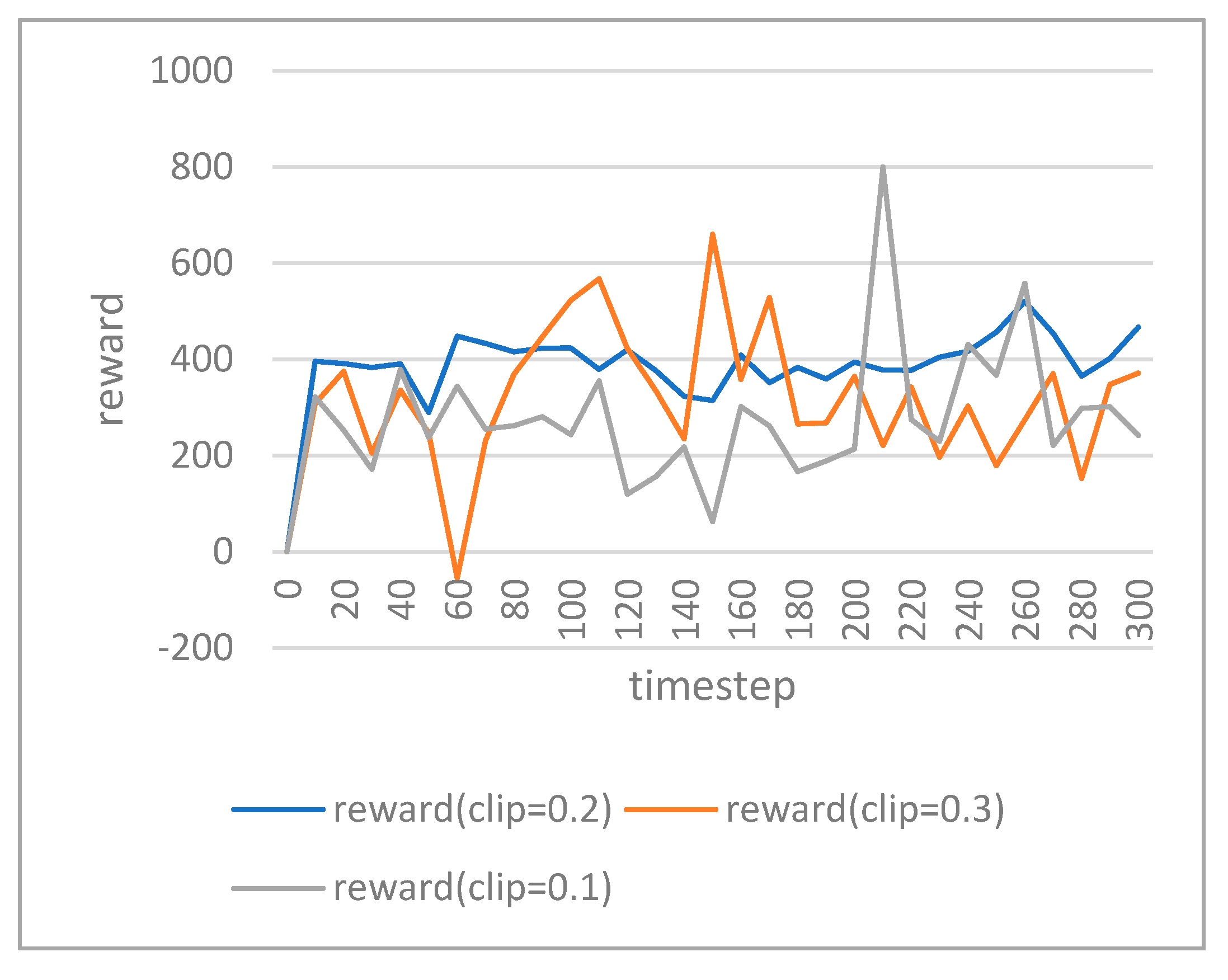
4.2. Training Performance

During the training process, we deployed 3000 pods over 300 training iterations. Each iteration consisted of ten timesteps, meaning that we deployed ten pods consecutively on a specific node during each step. This approach was implemented to amplify the impact of the action execution on the state input. Each pod ran a nginx application with a randomly assigned execution time to simulate different task execution effects. The lifecycle of the pod was determined by the task-execution period, and the pod would be automatically deleted upon task completion. We updated the policy every 30 steps during training and set the clipping parameter in the PPO algorithm to 0.2. The decay factor gamma was set to 0.99, and the learning rates for the actor and critic networks were set to 0.0003 and 0.001, respectively.

The average reward values during the training process are shown in Figure 5. The light-colored reward value curve represents the raw data, displaying a more accurate portrayal of the reward fluctuations, while the smoother reward value curve offers a clearer view of the average reward value’s increasing trend. The red curve corresponds to the reward values of the PPO-LRT algorithm, and the blue curve corresponds to the reward values of the default scheduling algorithm used by the Kube scheduler for the same scheduling training.

The average reward of the PPO-LRT algorithm rises rapidly within the first 0–50 steps, then increases at a slower pace within 50–200 steps, and finally approaches convergence after 300 training iterations. This demonstrates the advantage of the PPO algorithm in terms of the training convergence speed and stability. In contrast, the default scheduling algorithm exhibits significantly lower average rewards than the PPO-LRT and also displays a declining trend in the later stages. This phenomenon might be due to the Kube scheduler’s limitations in balancing the loads among different tasks and adapting swiftly to changes.

The clip parameter is an important hyperparameter used to limit the magnitude of policy updates. It plays a crucial role in maintaining the stability of policy updates while continually improving the policy in PPO. If the clipping parameter is set too small, policy updates may be overly constrained, resulting in slower convergence and requiring more training time to achieve the desired performance. Conversely, if the clipping parameter is set too large, policy updates may be too aggressive, leading to instability and divergence during training. This can result in excessive policy changes that prevent the effective learning of high-quality policies. Selecting an appropriate clipping parameter often requires experiments and hyperparameter tuning. Typically, an appropriate clipping parameter can be found to achieve fast, stable, and effective training. The reward curves trained with different clip parameters are shown in Figure 6. It can be observed that the clip parameter 0.2 results in more stable training and higher average reward values.

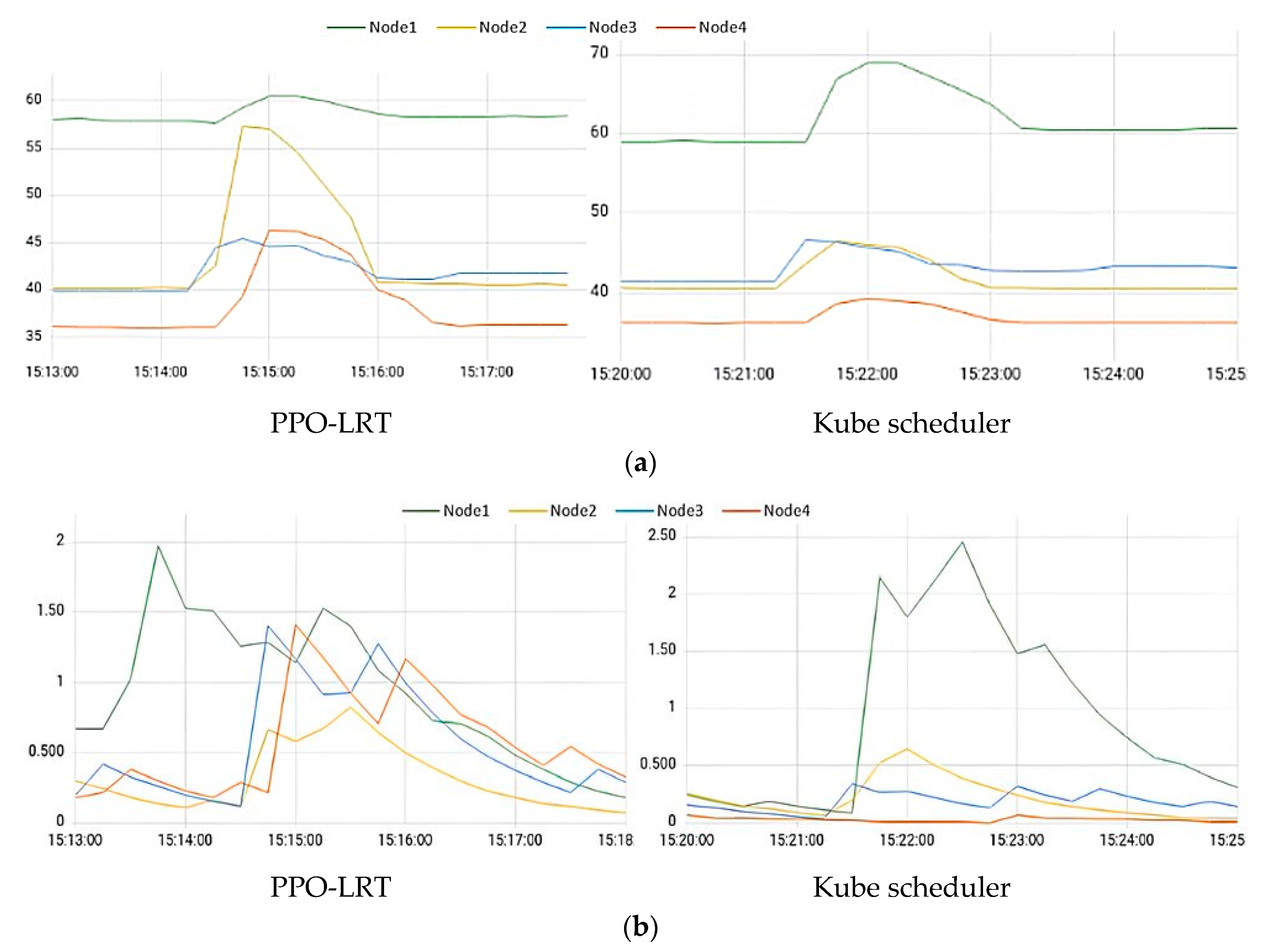
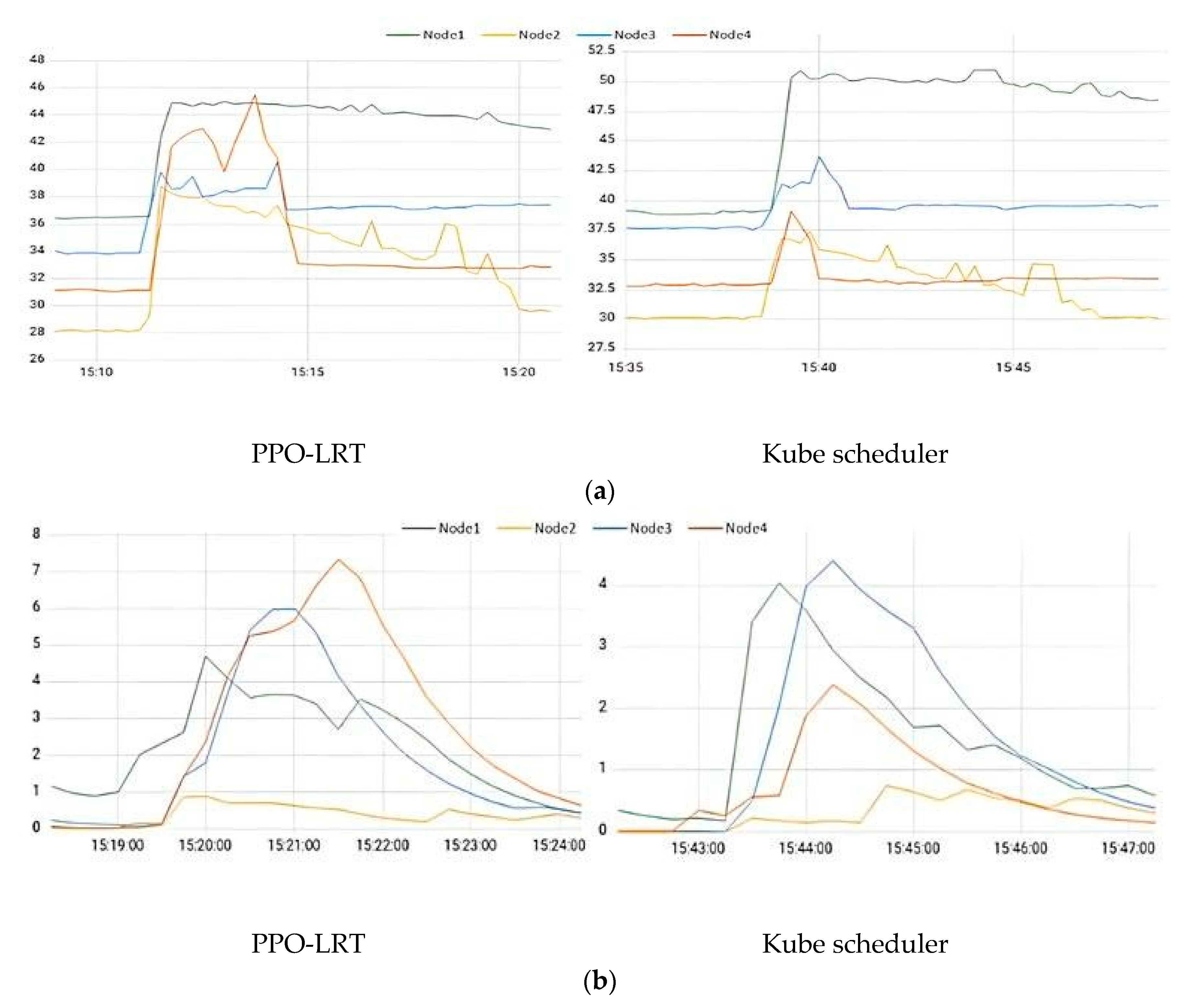
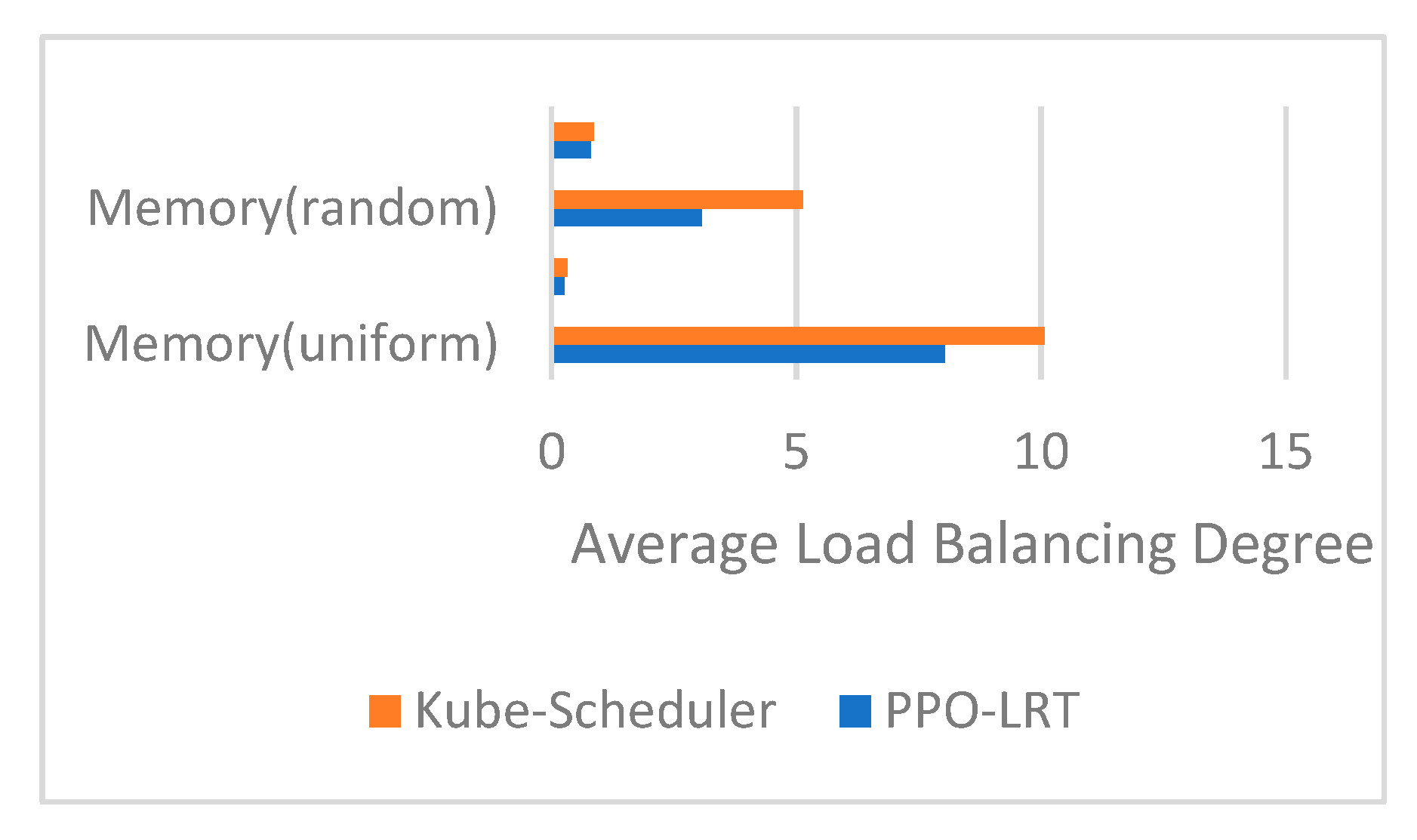
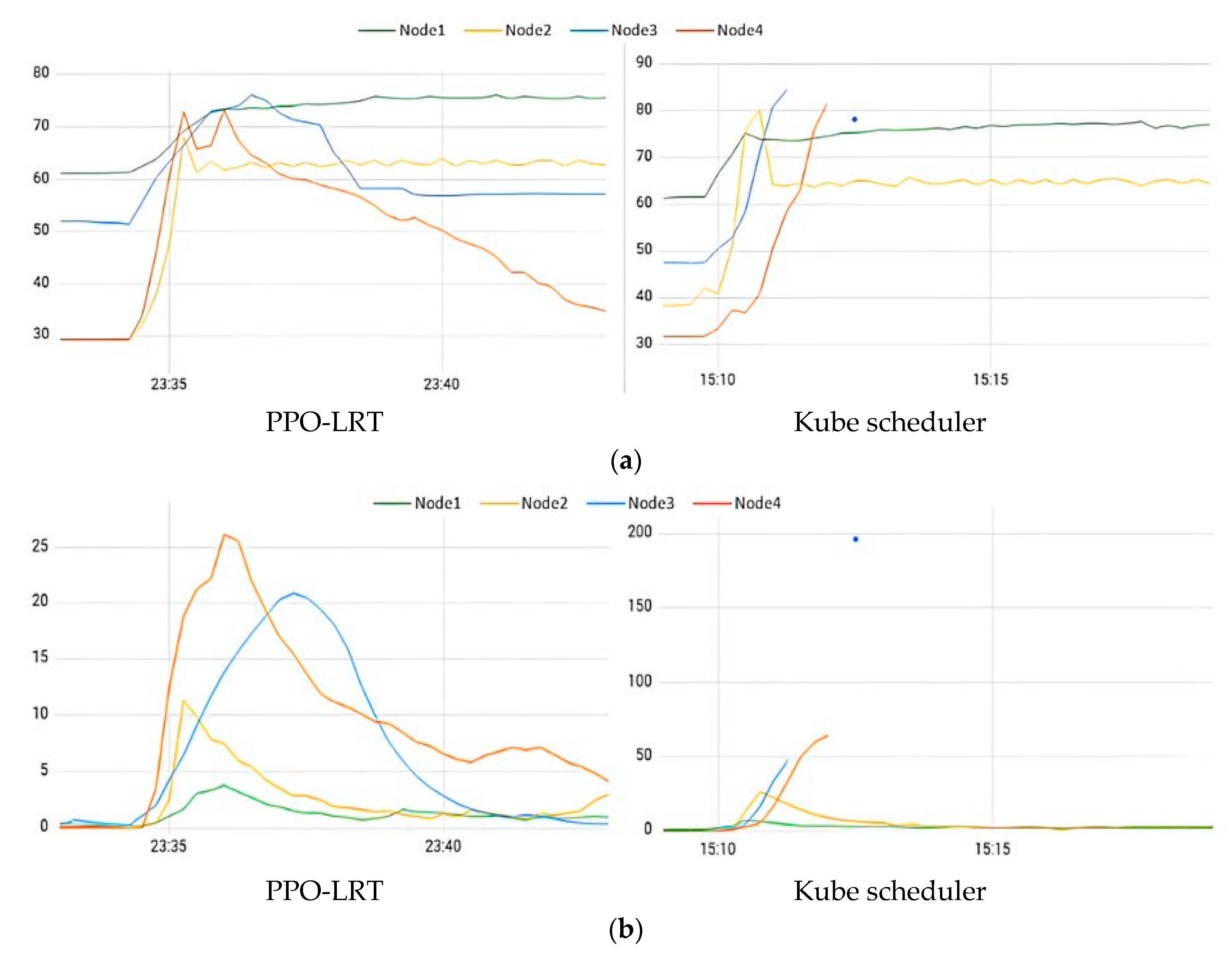
4.3. Load Balancing Test

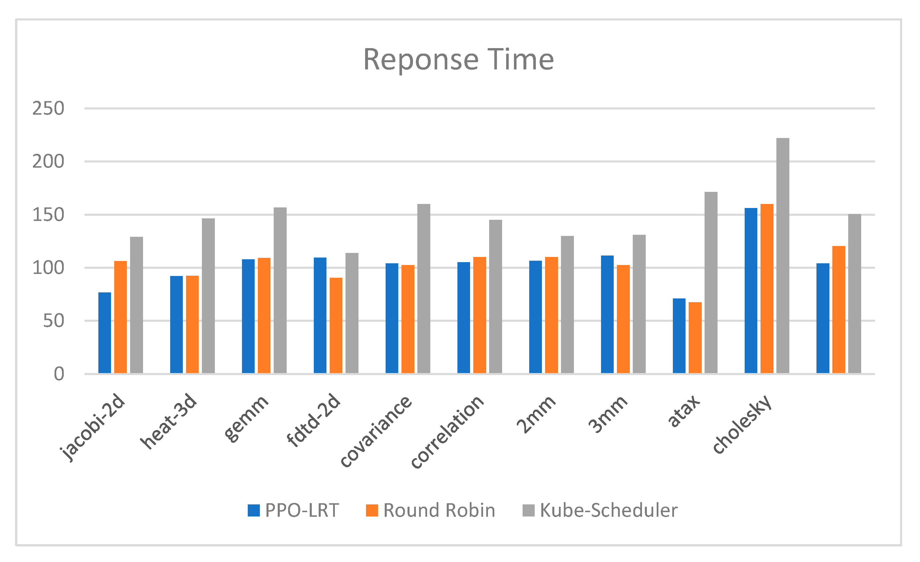
In edge clusters, workloads fluctuate unpredictably. A significant challenge for real-time task-scheduling optimization within the cluster is the ability to efficiently allocate and schedule a massive influx of tasks during peak workload periods. The aim is to prevent certain nodes from becoming overloaded, thereby averting blockage and a delayed task-response time. In this study, we employed both random and balanced workload test sets to determine if our PPO-LRT algorithm for edge Kubernetes clusters exhibits robust resilience under pressure and load-balancing optimization capabilities during peak workload scenarios. We compared its performance against the default Kube scheduler, and we also examined variations in the CPU and memory trends between the two schedulers throughout the test.

To recreate a peak workload environment, we deployed 100 Nginx applications for a uniform load test. Figure 7 illustrates the CPU and memory utilization patterns of the four nodes under this scenario. The closer the nodes’ curves align, the higher the level of load balancing within the cluster. As shown in Figure 7a, the PPO-LRT-scheduling results demonstrate effective load balancing under the circumstances of many applications being deployed quickly. The scheduler tends to allocate tasks to nodes with lower and more available resource utilization. Conversely, the default Kube scheduler tends to evenly allocate tasks among the four nodes, which may not be ideal. Node1′s memory load is already quite high before the test tasks arrive, but the Kube scheduler still assigns more tasks to it. Node1′s memory utilization is about 59% before the test tasks arrive. After deploying the test tasks, its memory utilization increases to about 69%. Node1 has the highest initial load, and its resource utilization increase is the highest among the four nodes, which can potentially lead to blocking. In Figure 7b, it is even more evident in the CPU load of each node in this situation. The number of tasks assigned to each node may not be evenly allocated with the PPO-LRT algorithm, but their overall loads are more balanced. In contrast, one node is overloaded with the Kube scheduler, which is a disadvantageous decision for the cluster.

Additionally, similar results are obtained in the random load test. We deployed 100 benchmarks at once, and each deployment randomly selected one program from the above 10 PolybenchC benchmarks. Random load testing is shown in Figure 8. It indicates that the scheduler with the PPO-LRT algorithm displays better load balancing, and CPU utilization is maintained at a relatively low level.

To demonstrate the advantages of the PPO-LRT algorithm more directly in terms of load balancing, we used Equation (8) as a measure of the load balance. Taking the CPU load as an example, during the testing period, we collected sample values at ten time points. We calculated the average load balance, denoted as average = $\sum _{t=1}^{10}{\sigma }_c^t/10$, which essentially represents the average standard deviation. Lower values indicate lower dispersion and a higher load balance. The same approach was applied to calculate the average memory load. We conducted tests by using two types of task sets: random and uniform. The four comparison scenarios are shown in Figure 9. In each scenario, we compared the load balance of the CPU and memory between cluster nodes when using the PPO-LRT and Kube scheduler for different types of tasks, respectively.

Further, we subjected the cluster to extreme task loads by deploying 500 pods with random tasks from PolybenchC during a brief period and recorded the CPU and memory trends of each node during the 10 min deployment. As shown in Figure 10, a normal cluster operation with relatively low load disparity among nodes was maintained by the PPO-LRT algorithm even under this high-pressure scenario, indicating sound-load balancing. However, memory loads of node3 and node4 exceed 80%, and CPU loads are around 50% when using the default scheduling algorithm of the Kube scheduler, which leads to interruptions in the status data, indicating that these nodes are blocked due to the high load.

4.4. Response Time

Response time is an important metric in real-time task scheduling in distributed clusters. It represents the total time taken for a task to be submitted to the cluster, executed, and the execution result returned to the user. A lower response time indicates that tasks can be executed faster, thereby improving the real-time performance of the system. Scheduling algorithms can prioritize nodes with shorter response times to execute tasks. It is to some extent a comprehensive reflection of the current cluster and node load status, as well as the network conditions. The goal of PPO-LRT is to balance the cluster load while taking into account the overall task-scheduling response time, maintaining the edge cluster in a good state for a longer period under resource-constrained and complex conditions, while providing faster and better services to clients.

To test the optimization effect of PPO-LRT on the response time, 10 selected PolybenchC benchmark programs from Table 3 were used. Each program was deployed 10 times by using both PPO-LRT and the default scheduler. After all the tasks were completed, the overall response time was recorded. Response time comparisons for real-time tasks with different algorithms are shown in Figure 11. PPO-LRT has a significant advantage in terms of response time compared to the Kube scheduler. According to the statistics, the average response time of all the tasks with PPO-LRT is 104.05 s, while the Kube scheduler had an average response time of 150.47 s. Overall, the PPO-LRT algorithm reduced the response time by approximately 31% compared to the Kube scheduler. However, when compared to the load-balancing round-robin scheduling algorithm with an average response time of 106.47 s, PPO-LRT’s response time is slightly improved by about 2.3%. The main reason is that the round-robin algorithm uses fixed round-robin scheduling, which evenly allocates tasks to the cluster in terms of quantity. However, this approach does not consider the initial load differences in the cluster. When the number of tasks is small, it can quickly allocate and execute them. When numerous tasks arrive in a short time and there are nodes with high loads in the cluster, this fixed strategy cannot adapt well to the situation and can easily lead to blockages in high-load nodes.

4.5. Results and Discussion

It is evident that the load difference among the nodes in the cluster using the PPO-LRT scheduler is significantly smaller than that of the Kube scheduler whether in a uniform load test or a random load test. This is because when designing the scheduling algorithm based on the PPO algorithm, we consider the standard deviation of the load values on each node as the most important measure in our reward function. If a node exceeds a reasonable load threshold, it incurs a penalty based on the actions from the previous scheduling round. Through this process, the scheduling strategy is trained to not only maintain load balance across the cluster but also to quantitatively measure load balance. The results indicate that PPO-LRT achieved the expected outcome. Furthermore, the LRT algorithm is employed to allocate different scores to each scheduling action based on its response time. The higher the score, the higher the reward during training, aiming to train strategies to respond faster. In summary, the above results demonstrate that PPO-LRT can bring superior load management and a faster response time to edge nodes.

The results also have a positive impact on three main areas: the edge environment efficiency, handling varying workloads, and providing a new optimization path for edge-task offloading. The proposed algorithm can improve the resource utilization to deal with limited and dynamically changing resources in edge-computing environments. As workloads continue to change with the increasing adoption of edge applications, it can adapt to the actual workload conditions, ensuring an effective cluster operation during a high-demand period. Finally, our research provides an effective way to manage and optimize Kubernetes clusters in edge environments and make task scheduling more scalable and maintainable.

5. Conclusions and Future Work

In edge environments, worker nodes lack the high computing power and capacity of cloud centers. Instead, they aim to provide faster and more secure computing services closer to the users. The nodes in an edge-computing cluster are often more dispersed and have limited computing resources. However, the unpredictable nature of tasks from IoT or vehicular networks, typical in edge-computing applications, challenges the cluster’s capacity. The solution lies in optimizing the task-scheduling algorithms, which must be in real time and dynamic for edge tasks. We tackled this problem by using deep reinforcement learning to enhance the Kubernetes pod-scheduling algorithm. First, the scheduling process is modeled by using Markov decision processes. Then, the PPO-LRT algorithm is designed. During batch-pod scheduling, the resource requirements, execution state, and cluster state changes are collected. The LRT algorithm is introduced into the reward function and the optimal scheduling policy network is obtained through actor–critic training. Finally, the scheduler based on PPO-LRT is tested by using the k3s framework. The results validate the superiority of our PPO-LRT-scheduling algorithm over the Kube scheduler in terms of the capacity during peak task-deployment periods, significantly improving load balancing across nodes in the cluster and reducing the likelihood of node blocking or crashes due to the workload. Furthermore, it improves the average execution speed by 31%.

However, there are still some limitations in our research. The single-agent algorithm used in our framework might not fully capture distributed decision-making capabilities. Kubernetes operates typically in a distributed environment with multiple nodes and clusters. Scheduling algorithms designed with a single intelligent agent may struggle to fully harness distributed decision-making capabilities and fail to consider communication and collaboration among nodes. It can be prone to local optima, especially in highly complex problems. Moreover, we designed our custom scheduler to be external, targeting improvements in maintainability and scalability. This design may introduce some network latency. Although the execution time of our algorithm is considered, providing some advantages over the default Kube scheduler, there is still room for optimization in terms of the network latency. These limitations suggest avenues for future research, such as exploring distributed reinforcement learning algorithms for Kubernetes scheduling in edge environments and further optimizing the network latency in custom schedulers.

We will continue to focus on task offloading and scheduling in a future study, aiming to design intelligent algorithms suitable for multinode coordinated scheduling, such as integrating multiagent reinforcement learning with edge multinode environments. Additionally, we will focus on improving the Kubernetes scheduling architecture, distributing decision-making authority to individual nodes to further boost cooperation and distributed processing capabilities during the task-scheduling decision-making process.

References

1. Wöbker, C.; Seitz, A.; Mueller, H.; Bruegge, B. Fogernetes: Deployment and management of fog computing applications. In Proceedings of the NOMS 2018—2018 IEEE/IFIP Network Operations and Management Symposium, Taipei, Taiwan, 23–27 April 2018; pp. 1–7. [Google Scholar]
2. Medel, V.; Tolón, C.; Arronategui, U.; Tolosana-Calasanz, R.; Bañares, J.Á.; Rana, O.F. Client-side scheduling based on application characterization on Kubernetes. In Proceedings of the Economics of Grids, Clouds, Systems, and Services: 14th International Conference, GECON 2017, Biarritz, France, 19–21 September 2017; Proceedings 14. Springer International Publishing: Berlin/Heidelberg, Germany, 2017; pp. 162–176. [Google Scholar]
3. Lai, W.K.; Wang, Y.C.; Wei, S.C. Delay-Aware Container Scheduling in Kubernetes. IEEE Internet Things J. 2023, 10, 11813–11824. [Google Scholar] [CrossRef]
4. Amirteimoori, A.; Tirkolaee, E.B.; Simic, V.; Weber, G.W. A parallel heuristic for hybrid job shop scheduling problem considering conflict-free AGV routing. Swarm Evol. Comput. 2023, 79, 101312. [Google Scholar] [CrossRef]
5. Goli, A.; Ala, A.; Hajiaghaei-Keshteli, M. Efficient multi-objective meta-heuristic algorithms for energy-aware non-permutation flow-shop scheduling problem. Expert Syst. Appl. 2023, 213, 119077. [Google Scholar] [CrossRef]
6. Kchaou, H.; Kechaou, Z.; Alimi, A.M. A PSO task scheduling and IT2FCM fuzzy data placement strategy for scientific cloud workflows. J. Comput. Sci. 2022, 64, 101840. [Google Scholar] [CrossRef]
7. Park, S.; Jeon, J.; Jeong, B.; Park, K.; Baek, S.; Jeong, Y.S. Actual Resource Usage-Based Container Scheduler for High Resource Utilization. In Proceedings of the International Conference on Computer Science and Its Applications and the International Conference on Ubiquitous Information Technologies and Applications, Vientiane, Laos, 19–21 December 2022; Springer Nature Singapore: Singapore, 2022; pp. 611–614. [Google Scholar]
8. Harichane, I.; Makhlouf, S.A.; Belalem, G. KubeSC-RTP: Smart scheduler for Kubernetes platform on CPU-GPU heterogeneous systems. Concurr. Comput. Pract. Exp. 2022, 34, e7108. [Google Scholar] [CrossRef]
9. Menouer, T. KCSS: Kubernetes container scheduling strategy. J. Supercomput. 2021, 77, 4267–4293. [Google Scholar] [CrossRef]
10. Shi, B.; Chen, F.; Tang, X. Deep Reinforcement Learning Based Task Offloading Strategy Under Dynamic Pricing in Edge Computing. In Proceedings of the International Conference on Service-Oriented Computing, Online. 22–25 November 2021; Springer International Publishing: Cham, Switzerland, 2021; pp. 578–594. [Google Scholar]
11. Yamansavascilar, B.; Baktir, A.C.; Sonmez, C.; Ozgovde, A.; Ersoy, C. Deepedge: A deep reinforcement learning based task orchestrator for edge computing. IEEE Trans. Netw. Sci. Eng. 2022, 10, 538–552. [Google Scholar] [CrossRef]
12. Xiao, L.; Lu, X.; Xu, T.; Wan, X.; Ji, W.; Zhang, Y. Reinforcement learning-based mobile offloading for edge computing against jamming and interference. IEEE Trans. Commun. 2020, 68, 6114–6126. [Google Scholar] [CrossRef]
13. Lim, D.; Joe, I. A DRL-Based Task Offloading Scheme for Server Decision-Making in Multi-Access Edge Computing. Electronics 2023, 12, 3882. [Google Scholar] [CrossRef]
14. Xu, X.; Liu, K.; Dai, P.; Jin, F.; Ren, H.; Zhan, C.; Guo, S. Joint task offloading and resource optimization in noma-based vehicular edge computing: A game-theoretic drl approach. J. Syst. Archit. 2023, 134, 102780. [Google Scholar] [CrossRef]
15. Zhao, N.; Ye, Z.; Pei, Y.; Liang, Y.C.; Niyato, D. Multi-agent deep reinforcement learning for task offloading in UAV-assisted mobile edge computing. IEEE Trans. Wirel. Commun. 2022, 21, 6949–6960. [Google Scholar] [CrossRef]
16. Agarwal, S.; Rodriguez, M.A.; Buyya, R. A reinforcement learning approach to reduce serverless function cold start frequency. In Proceedings of the 2021 IEEE/ACM 21st International Symposium on Cluster, Cloud and Internet Computing (CCGrid), Melbourne, Australia, 10–13 May 2021; pp. 797–803. [Google Scholar]
17. Huang, J.; Xiao, C.; Wu, W. Rlsk: A job scheduler for federated kubernetes clusters based on reinforcement learning. In Proceedings of the 2020 IEEE International Conference on Cloud Engineering (IC2E), Sydney, Australia, 21–24 April 2020; pp. 116–123. [Google Scholar]
18. Peng, Y.; Bao, Y.; Chen, Y.; Wu, C.; Meng, C.; Lin, W. Dl2: A deep learning-driven scheduler for deep learning clusters. IEEE Trans. Parallel Distrib. Syst. 2021, 32, 1947–1960. [Google Scholar] [CrossRef]
19. Burns, B.; Beda, J.; Hightower, K.; Evenson, L. Kubernetes: Up and Running; O’Reilly Media, Inc.: Sebastopol, CA, USA, 2022. [Google Scholar]
20. Carrión, C. Kubernetes scheduling: Taxonomy, ongoing issues and challenges. ACM Comput. Surv. 2022, 55, 1–37. [Google Scholar] [CrossRef]
21. Rejiba, Z.; Chamanara, J. Custom scheduling in Kubernetes: A survey on common problems and solution approaches. ACM Comput. Surv. 2022, 55, 1–37. [Google Scholar] [CrossRef]
22. Arulkumaran, K.; Deisenroth, M.P.; Brundage, M.; Bharath, A.A. Deep reinforcement learning: A brief survey. IEEE Signal Process. Mag. 2017, 34, 26–38. [Google Scholar] [CrossRef]
23. Schulman, J.; Wolski, F.; Dhariwal, P.; Radford, A.; Klimov, O. Proximal policy optimization algorithms. arXiv 2017, arXiv:1707.06347. [Google Scholar]
24. Kakade, S.; Langford, J. Approximately optimal approximate reinforcement learning. In Proceedings of the 19th International Conference on Machine Learning, Sydney, Australia, 8–12 July 2002. [Google Scholar]
25. Arshad, A. What Is the Least Response Time Load Balancing Technique. Available online: https://www.educative.io/answers/what-is-the-least-response-time-load-balancing-technique (accessed on 30 December 2021).
Figure 1. Kubernetes cluster architecture.
Mathematics 11 04269 g001
Figure 2. Schematic of Kubernetes scheduler based on PPO-LRT algorithm.
Mathematics 11 04269 g002
Figure 3. Time-sequence diagram of PPO-LRT training.
Mathematics 11 04269 g003
Figure 4. Flowchart of PPO algorithm.
Mathematics 11 04269 g004
Figure 5. The average reward values during the training process.
Mathematics 11 04269 g005
Figure 6. Training results for different clip parameters.
Mathematics 11 04269 g006
Figure 7. Uniform load testing. (a) Memory comparisons with uniform load; (b) CPU comparisons with uniform load.
Mathematics 11 04269 g007
Figure 8. Random load testing. (a) Memory comparisons with random load; (b) CPU comparisons with random load.
Mathematics 11 04269 g008
Figure 9. Average load balancing comparisons.
Mathematics 11 04269 g009
Figure 10. High load testing. (a) Memory comparisons with high load; (b) CPU comparisons with high load.
Mathematics 11 04269 g010
Figure 11. Response time comparisons for real-time tasks with different algorithms.
Mathematics 11 04269 g011